HQ-Modellflugliteratur On the Longitudinal Stability of Gliders

135 

Dr. Helmut Quabeck 

Finkenweg 39 

64832 Babenhausen 

Germany 

HQ-Modellflugliteratur 

On the Longitudinal Stability of Gliders 

By Helmut Quabeck, © 

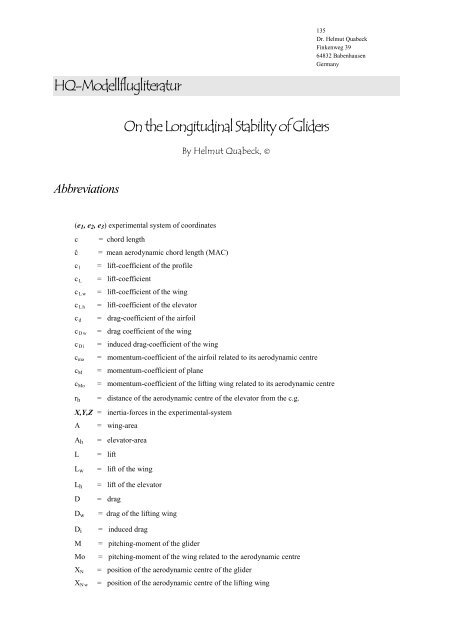
Abbreviations 

(e 1 , e 2 , e 3 ) experimental system of coordinates 

c = chord length 

ĉ = mean aerodynamic chord length (MAC) 

c l 

c L 

c L w 

c L h 

c d 

c D w 

c D i 

c mo 

c M 

c Mo 

r h 

= lift-coefficient of the profile 

= lift-coefficient 

= lift-coefficient of the wing 

= lift-coefficient of the elevator 

= drag-coefficient of the airfoil 

= drag coefficient of the wing 

= induced drag-coefficient of the wing 

= momentum-coefficient of the airfoil related to its aerodynamic centre 

= momentum-coefficient of plane 

= momentum-coefficient of the lifting wing related to its aerodynamic centre 

= distance of the aerodynamic centre of the elevator from the c.g. 

X,Y,Z = inertia-forces in the experimental-system 

A = wing-area 

A h = elevator-area 

L = lift 

L w = lift of the wing 

L h 

D 

D w 

D i 

M 

Mo 

X N 

X N w 

= lift of the elevator 

= drag 

= drag of the lifting wing 

= induced drag 

= pitching-moment of the glider 

= pitching-moment of the wing related to the aerodynamic centre 

= position of the aerodynamic centre of the glider 

= position of the aerodynamic centre of the lifting wing

Xc.g. = position of the centre of gravity 

V = velocity of the glider 

α = angle of attack 

α w 

ε 

ά 

h 

ε 

Λ w 

a w 

= downwash-angle 

= difference of the angles of incidence of elevator and wing 

= dα/dt rotational speed of the angle of attack 

= angle of inclination, gliding-angle 

= difference of angles of incidence 

= aspect-ratio of the wing 

= lift efficiency-factor of the lifting wing 

a p (α) = airfoil efficiency-factor of the lifting wing 

a w 

x 

= efficiency-factor of the lifting wing, a w 

x = aw @ a p (α) 

Λ h 

a h 

= aspect-ratio of the elevator (shape influence) 

= lift efficiency-factor of the elevator (shape-influence) 

q 

= ω y = rotational speed around the lateral y-axis through the c.g. 

q = aerodynamic pressure, q = ρ/2 @ V 2 

ρ 

σ 

m 

m i 

r i 

J y 

J yi 

F(n) 

λ 1;2 

λ 3;4 

= airdensity, ≈1.25 kg/m 3 at sea-level 

= measure of the static stability 

= body-mass 

= mass of model part i (e.g. wing, fuselage, elevator,…) 

= distance of the mass-centre of model-part i from the c.g. 

= mass-moment of inertia related to y-axis (c.g.) 

= mass-moment of inertia of model-part i related to y-axis (c.g.) 

= characteristic equation with n solutions 

= solutions of F(4) for α-disturbances- 

= solutions of F(4) for ϑ-V-disturbances 

--- 

2

1. General Determinations 

Generally in this paper for all theoretical considerations the so-called experimental system (e 1 , e 2 , e 3 ) of 

coordinates will be chosen , where e 1 coincides with the gliding path of the model and has an angle h of 

inclination against the geodetic horizon. e 2 is chosen horizontally and coincides with the lateral-y-axis of 

the glider in wing direction, and e 3 is defined by e 3 = e 1 x e 2. 

The angle of attack α of the wing thus is related to the axis e 1. 

The angles α and h generally can vary independent on each other and consequently also their time 

derivatives ά = dα/dt and q = ω y = dh/dt. 

Consequently the direction of the gliding speed V points towards the negative direction of the e 1 –axis. 

2. Forces at the Glider at longitudinal Motion 

In the experimental system of coordinates the equations of the forces acting at a glider, namely the forces 

due to mass inertia and the aerodynamic lift and drag forces, are 

e 1 – direction: 

X 

X 

= m ⋅V& 

= −m 

⋅ g ⋅sinϑ 

− D 

(2.1) 

– e 3 – direction: 

Z = m ⋅V 

⋅ϑ& 

Z = −m 

⋅ g ⋅ cosϑ 

+ L 

(2.2) 

3. Pitching-Moment of the Glider 

The pitching-moment M caused by air forces at the glider in general depends on 

the angle of attack α, 

the rotational speed of the angle of attack ά = dα/dt , 

and the rotational speed around the y-axis (lateral axes) q = ω y 

M = M(α, ά, ω y ) (3.1) 

Using a non-dimensional momentum coefficient c m , according to aerodynamic theory we get 

M = c m (α, ά, ω y )@ q @ A@ ĉ (3.2) 

Taylor development of the momentum-coefficient c m provides 

c 

m 

α& 

⋅ cˆ 

V 

y 

= c 

m 

( α ,0 ,0 ) + ⋅ c 

m , α& 

+ ⋅ c 

m , ω 

ω 

V 

⋅ cˆ 

y 

(3.3) 

Therein the derivatives c m ά = ∂ c m /∂ά and c m ωy = ∂ c m /∂q are dependent on α. 

3

The second term signifies the coefficient of a damping-moment which is proportional to the rotational 

speed ά . Essentially it results from the fact that the angle α w (t) of the downwash resulting from the lifting 

wing at the elevator in case of ά à 0 does not correspond to the angle of attack α(t) of the wing, but to 

the angle α(t + ∆t). ∆t ≈ r h /V and r h is about the distance of the aerodynamic centre of the elevator 

from the centre of gravity, c.g. E.g. for ά > 0 the downwash angle α w gets smaller and the resulting 

angle of attack at the elevator becomes α h = α (t) - α w (t + ∆t). Thus the lift at the elevator becomes 

larger then for the stationary case with ά = 0, a negative pitching-moment will result, and in general we 

have c mά < 0. 

The third term signifies the coefficient of a dampening-moment which is proportional to the rotational 

speed q = ω y around the lateral axis through the c.g. It results from the fact that the angle of attack and 

thus the lift at the elevator in case of ω y > 0 is increased by the angle ω y @ ĉ/V as compared to the 

stationary state with ω y = 0. Again a negative pitching-moment results with c mωy < 0. 

These aerodynamic pitching-moments are counteracted by the mass-inertia of the glider-parts expressed 

by their moments of inertia J y around the y-axis of the glider. May m i be the mass of a glider part and r i its 

distance from the c.g., then the mass-moment of inertia of the glider can roughly be assessed to be 

J 

y 

= ∑ m ⋅ r 

i 

Thus for the pitching moment generally we have 

M = J 

y 

i 

2 

i 

2 2 

∂ ϑ ∂ α 

⋅ ( + ) = J 

2 2 

∂t 

∂t 

y 

∂q 

∂ & α 

⋅ ( + ) 

∂t 

∂t 

(3.4) 

(3.5) 

4. Aerodynamic Centre of the Glider, XN X 

The aerodynamic centre of the glider is defined as the point X N on its longitudinal axis about which the 

pitching moment is constant with respect to the angle of attack. Thus in case of a change of the angle of 

attack the resulting Lift L will act through X N . 

Equally the aerodynamic centre of the lifting wing is defined as the point X Nw about which the pitching 

moment of the wing, in generally dependent on the wing-shape and the properties of the chosen airfoils, is 

constant with respect to the angle of attack. Since the lift- and momentum-characteristics, c l (α) and 

c m (α), of most airfoils show a slightly non-linear dependence on the angle of attack for low Reynoldnumbers, 

Re < 1@10 6 , the aerodynamic centre of model-wings can only be considered to be stable for 

small α-ranges. This has to be taken into account at the design of a model-plane in order to achieve 

proper static and dynamic flight behaviour under all flight conditions. 

The displacement of the overall aerodynamic centre of the plane X N vs. the aerodynamic centre of the 

wing X Nw may be denoted by ∆X N = X N - X Nw . The momentum-equilibrium of the plane is then given 

by 

∆X N @ L = r Nh @ L h (4.1) 

Herein L h is the contribution of the elevator to the overall lift of the plane, and r Nh is the distance of the 

aerodynamic centres of lifting wing and elevator. According to aerodynamic theories we get 

L h = c lh @ A h @ q h (4.2) 

c lh is the lift coefficient of the elevator related to the area A h of the elevator and the aerodynamic 

pressure q h at the location of the elevator. For practical reasons it is preferred to relate the lift coefficient 

of the elevator to the wing area A and its aerodynamic pressure q : 

L h = c Lh @ A @ q (4.3) 

4

By comparison one gets 

c Lh = c lh @ A h /A @ q h /q (4.4) 

If the airflow on the elevator would not be influenced by the wake from the wing we would get the 

derivative 

c 

Lh ,α 

∂ c 

Lh 

∂ c 

lh 

= ⋅ α = ⋅ α ⋅ 

∂ α ∂ α 

q 

⋅ 

q 

However, since downwash w is generated in the wake of the wing, the angle of attack at the elevator 

location is reduced by the downwash angle α w = w/V. The difference of the angles of incidence between 

wing and elevator may be denoted by ε , then the angle of attack at the elevator is given by 

(4.5) 

α h = α + α w + ε (4.6) 

Taking this angle of attack into account, the coefficient of the elevator lift results to be 

A 

h 

A 

h 

c 

Lh 

= c ⋅ ( α + α + ) ⋅ 

lh , α 

w 

ε 

A 

h 

A 

⋅ 

q 

q 

h 

(4.7) 

At a disturbance of the longitudinal motion of the plane around the pitching-axis with fixed rudder the 

change of the elevator lift coefficient with α is given by the derivative c Lh, α : 

c 

Lh , α 

d α 

w 

= c 

lh , α 

⋅ (1 + ) ⋅ 

d α 

A 

h 

A 

q 

⋅ 

q 

h 

(4.8) 

The overall lift-coefficient is 

c L = c Lw + c Lh (4.9) 

and in case of a disturbance around the pitching axis the lift-slope c L,α of the whole plane in case of fixed 

controls results to 

c 

L , α 

d α 

w 

= c 

Lw , α 

+ c 

lh , α 

⋅ (1 + ) ⋅ 

d α 

Ah 

A 

q 

⋅ 

q 

h 

(4.10) 

Using formulas 4.8 and 4.10 in formula 4.1, we will receive 

∆ X 

N 

= 

c 

c 

Lh , α 

L , α 

⋅ r 

Nh 

(4.11) 

Related to the mean aerodynamic chord of the wing finally results 

∆X 

cˆ 

N 

= 

c 

Lw 

dα 

w 

Ah 

qh 

clh, 

α 

⋅ (1 + ) ⋅ ⋅ 

dα 

A q 

dα 

w 

Ah 

qh 

, α 

+ clh, 

α 

⋅ (1 + ) ⋅ ⋅ 

dα 

A q 

r 

⋅ 

cˆ 

Nh 

(4.12) 

In a larger distance behind the wing the free vortices of both halves of the wing induce a downwash 

angle of about α w∞ = −2 c Lw / (π @ Λ w ). There from results ∂ α w∞ / ∂ α = − 2 c Lw,α / (π @ Λ w ) and for the 

aerodynamic centre of the plane 

5

∆X 

c 

= 

c 

2cLw, 

α Ah 

qh 

clh, 

α 

⋅ (1 − ) ⋅ ⋅ 

π ⋅ Λ 

w 

A q 

2cLw 

α Ah 

qh 

, α 

+ clh, 

α 

⋅ (1 − ) ⋅ ⋅ 

π ⋅ Λ A q 

N 

ˆ , 

Lw 

w 

r 

⋅ 

cˆ 

Nh 

(4.13) 

This formula is still rather complex and for most modellers impossible to solve. A way out of this 

dilemma is found for practical cases when considering how the derivatives c Lw,α and c lh,α depend on the 

lifting characteristics of the chosen airfoils and on the shape of wing and elevator. 

The slope of the lift-coefficient of a lifting wing, namely c Lw,α , is closely related to the slope of the liftcoefficient 

of the applied airfoil, namely c l,α by an efficiency factor denoted as a w 

c Lw,α = a w @ c l,α (4.14) 

a w takes into account the influence of the wing-shape on the formation of the free vortices on the wingsurfaces. 

According to the limited wing-span and the wing-shape the ideal lifting-efficiency of the airfoil 

is reduced. In an ideal non-viscous environment the slope of an ideal airfoil would be c l,α = 2@π. However, 

in a viscous airflow for Re-numbers below 1@10 6 non-linear deviations from this ideal slope may be 

experienced, in the practically non-critical range of the angles of attack mostly an increase up to 5% are 

experienced. This can be taken into account by another efficiency-factor a p (α), Thus we get 

c Lw,α = a w @ a pw (α) @ 2@π (4.15) 

c lh,α = a h @ a ph (α) @ 2@π (4.16) 

Denoting a x = a w @ a p (α) formula 2.13 after a few rearrangements can be rewritten to a practically easier 

form: 

∆X 

cˆ 

N 

× × 

aw 

⋅ ah 

⋅ Ah 

A r 

= 

⋅ 

× × 

1+ 

a ⋅ a ⋅ A A cˆ 

w 

h 

h 

Nh 

(4.17) 

therein a w and a h denote the total lifting-efficiencies of wing and elevator. 

Remark: The lifting efficiency factors a w and a h can easily be determined by means of the “FMFM”- 

program of the author. 

For many practical cases it is sufficient to approximately chose a p .1, and if the aspect-ratio Λ $ 5 then 

according to the expanded lifting line theory the efficiency-factors can be approximated by 

× 

a 

= Λ (2 + 

Λ 2 + 4) 

(4.18) 

According to long time experience, using this approach very reliable result of flight-stability could be 

practically achieved, as will be explained by an example later on. 

5. Static longitudinal stability, σ 

One of the most important flight mechanical characteristics of a glider is the capability, to redress the 

balance of the original stationary longitudinal flight state after disturbance of the angle of attack by ∆α 

without using controls. A disturbance of the angle of attack causes an increase or decrease of the lift by 

∆L of the plane, if thereby a momentum ∆M is caused that forces the plane to rotate back to the original 

state, the plane is featured statically stable. Thus a glider behaves statically stable if generally holds true 

that 

6

dM = −σ @ dL (5.1) 

σ is a non-dimensional positive constant factor which is considered as a stability-measure for the 

stationary longitudinal flight of a glider. The larger it is, the larger the back-leading momentum will be. 

For σ = 0 the stability-behaviour of the plane will be indifferent and it will no more be controllable, for σ 

< 0 the longitudinal flight of the plane will become instable. 

Note: As will be shown later, besides σ also the mass-moments of inertia Jy of the glider parts are to be 

taken into account to completely determine the time-dependent motion of a glider back to flight-balance 

after disturbance. 

Using non-dimensional aerodynamic coefficients we get 

σ = − dc M / dc L (5.2) 

Based on the explanations in chapter 2 the pitching moment around the c.g. is given by 

M = −(X N − X c.g. )@ L + M ow − r h @ A h + M oh (5.3) 

Therein M ow is the pitching-moment for the wing at the aerodynamic centre, M oh is that of the elevator, 

and r h is the distance of the aerodynamic centre of the elevator from c.g. Moments according to the 

vertical position of the forces can mostly be neglected for gliders. For the change of the pitching-moment 

around the c.g. by change of the lift here from results 

dc M / dc L = −(X N −X c.g. ) / ĉ (5.4) 

Implementing (3.4) in (3.2) yields 

σ = (X N −X c.g. ) / ĉ (5.5) 

Therewith we have a very useful, quantitative measure for the static stability of the glider, namely the 

distance of the c.g. from the aerodynamic centre of the plane related to the mean aerodynamic chord of 

the lifting-wing. Because of the requirement σ > 0, the c.g. must be positioned in front of X N in order to 

achieve longitudinal static flight stability. 

As will be discussed in more detail later on, usually the position of the centre of gravity is to be chosen 

such that the lift coefficient c L at slow stationary gliding is either adapted to the optimum gliding or to the 

minimum sinkrate. Once the c.g. is determined by evaluation of the profile- and wing-characteristics, by 

means of the theoretical considerations in chapter 4 the geometrical parameters of the glider can be 

chosen such that the required size of σ will be achieved. One problem here may be how it can be found 

out what the appropriate size of σ is. The most adequate way is to determine the static stability of one or 

more representative models which are considered to have good stability-behaviour. 

6. Free Oscillations of a Glider with Fixed Controls 

The static stability-measure σ in principle just provides an answer to the question whether or not a glider 

will behave stable on a stationary linear flight path. However, it does not inform how fast the glider will 

redress the original stationary balance after any disturbance. In case of static stability we can expect that 

the glider performs attenuated oscillations. In the most general case a glider may conduct combined α- 

and h-oscillations as well as oscillations of the c.g along the gliding path. As will be outlined later on, in 

most practical cases the α-oscillations are much faster than the c.g.-oscillations and by means of 

appropriate choice of the glider-design-parameters it can be achieved, that these oscillations are damped 

to such a degree that the glider returns to balance in a very short time. c.g.-oscillations take longer and 

cannot so well be damped, however, in practice they can easily be balanced out by proper RC-controlling 

of the pilot. 

In order to determine the behaviour of a glider after disturbance of the angle of attack and/or the gliding 

angle this movements may be considered as small disturbances ∆V, ∆α und ∆h of a stationary linear 

7

flight path. Then the equations for the forces at the glider, given in chapter 2, may be developed into 

Taylor-progressions whereby higher power elements are neglected: 

m ⋅V& 

= X 

V 

⋅ ∆V 

+ X 

ϑ 

⋅ ∆ϑ 

+ X 

α 

⋅ ∆α 

X V 

= − ∂D 

∂V 

Xα = −∂D 

∂α 

Xϑ = −m⋅ 

g ⋅ cosϑ 

(6.1) 

and 

m ⋅V 

⋅ϑ& 

= Z 

V 

⋅ ∆V 

+ Z 

ϑ 

⋅ ∆ϑ 

+ Z 

α 

⋅ ∆α 

Z V 

= ∂L 

∂V 

Zϑ = m ⋅ g ⋅sinϑ 

Zα = ∂L 

∂α 

(6.2) 

Equally the momentum equation of chapter 3 is developed to 

J 

2 

2 

d ∆ϑ 

d ∆α 

⋅ ( + = M 

2 

2 

dt dt 

y 

) 

V 

⋅ ∆V 

+ M 

α 

⋅ ∆α 

+ M 

& ϑ 

⋅ & ϑ + M 

& α 

⋅ & α 

M V 

= ∂M 

(α,0,0) 

∂V 

⋅ q ⋅ A⋅ 

c 

M 

= ∂M 

( α,0,0 

∂α 

⋅ q ⋅ A⋅ 

c 

α 

) 

M c V ⋅ cm ⋅ q ⋅ A⋅ 

c 

& = 

ϑ , ω 

(6.3) 

M 

& α 

= c V ⋅ c + c ) ⋅ q ⋅ A⋅ 

c 

( 

m, & α m, 

ω 

Rearrangement of the force equations 6.1 and 6.2 and of the momentum equation 6.3 provides 

( m ⋅ 

d 

dt 

− Z 

− M 

− X 

V 

V 

V 

⋅ ∆V 

⋅ ∆V 

) ∆V 

+ ( m ⋅V 

⋅ 

+ ( J 

y 

− X 

d 

⋅ 

dt 

ϑ 

d 

dt 

2 

2 

⋅ ∆ϑ 

− Z 

− M 

ϑ 

& ϑ 

) ∆ϑ 

) ∆ϑ 

+ ( J 

y 

d 

⋅ 

dt 

2 

2 

− X 

− Z 

α 

α 

− M 

⋅ ∆α 

⋅ ∆α 

& α 

⋅ 

d 

dt 

− M 

α 

= 0 

= 0 

= 0 

) ∆α 

(6.4) 

By means of an exponential description of the disturbances according to 

∆V = ∆V o @ e λt , 

∆α = ∆α o @ e λt , ∆h = ∆h o @ e λt 

the characteristic equation of the system F 4 (λ) becomes: 

m ⋅ λ − X 

V 

− X 

ϑ 

− X 

α 

m 

2 

⋅V 

⋅ J 

y 

⋅ F ( λ) 

≡ 

4 

− Z 

V 

m ⋅Vλ 

− Z 

ϑ 

− Z 

α 

(6.5) 

− M 

V 

2 

Jy ⋅ λ − M 

& ϑ 

⋅ λ 

J 

y 

2 

⋅ λ − M 

& α 

⋅ λ − M 

α 

8

In flight-mechanical theories this equation is usually written in subsequent form 

λ 4 + B @ λ 3 + C @ λ 2 + D @ λ + E = 0 (6.6) 

According to the stability criteria of Hurwitz for an oscillating system like the one considered 

E > 0 ! (6.7) 

is a necessary requirement for the longitudinal stability of the glider. Taking equations 6.1 to 6.3 into 

account, in detail we get 

2 ∂D 

∂L 

∂L 

∂D 

m VJ ⋅ E = ( mg sinϑ 

− mg cosϑ) 

M + ( mg cosϑ 

− mg sinϑ) 

∂V 

∂V 

∂α 

∂α 

y α 

M V 

(6.8) 

This can be rewritten to 

2 

m VJ 

y 

⎡ 

∂ 

⎢ 

⋅ E = − ( L ⋅ mg cosϑ 

− D ⋅ mg sinϑ) 

⋅ 

∂ 

⎢M 

V 

⎢ 

⎣ 

α 

+ M 

V 

∂ 

⎤ 

( L ⋅ mg cosϑ 


∂α 

⎥ 

∂ 

⎥ 

( L ⋅ mg cosϑ 


⎥ 

∂V 

⎦ 

Here from results 

∂ 

− ( L ⋅ mg cosϑ 


∂ 

⎡ 

E = V 

⋅ 

⎢ 

M 

2 

m VJ 

⎣ 

y 

α 

+ M 

V 

δV 

⎤ 

⋅ 

δα ⎥ 

⎦ 

(6.9) 

Under normal angles of attack ∂L/∂V@m@g@cosh - ∂D/∂V@m@g@sinh > 0, thus the requirement 6.7 is 

identical with the requirement 

⎡ 

− 

⎣ 

⎢ 

M 

α 

+ M 

V 

δV 

⎤ 

⎥ 

≥ 0 

δα ⎦ 

(6.10) 

δV/δα denotes the deviation of the speed by α, therefore the differential-quotient of the overall pitchingmoment 

M derived by α and taken along the speed polar must be negative in order to achieve static 

longitudinal stability: 

−δM/δα > 0 (6.11) 

This result is well in correspondence with those of chapter 5. 

6.1 Fast pitching-oscillations 

At stationary free flight gliding under condition 6.11 for static longitudinal stability, because of the 

requirements ∆ V = ∆h = 0 the characteristic equation 6.5 will be reduced to 

J y 

2 

⋅ λ − M 

& α 

⋅ λ − M 

α 

= 0 

(6.1.1) 

This is the characteristic equation of an attenuated pitch-oscillation around the c.g. Since the attenuation 

factor −M ά is always positive by nature, this equation provides real roots in case of stability with 

−M α >0. By means of equations 6.3 we get 

9

J 

y 

2 

⋅λ 

− 

c 

V 

( cm, 

& 

+ cm, 

y 

) ⋅ q ⋅ A⋅cˆ 

⋅λ 

− cm, 

α 

ω 

α 

⋅ q ⋅ A⋅cˆ 

= 0 

(6.1.2) 

In order to solve this equation, next the derivatives herein have to be determined. 

6.1.a The q-derivative 

q 

Dependent on the rotation of the glider around the lateral axis y with the angular speed q = ω y , the so 

called q-derivatives, will play a roll. They result from the distinct air wash which emerges at the various 

parts of the glider by interference of the general airflow with speed V and of the local vertical air flow 

with speed q @ r = ω y @ r of the rotation, and where r is the distance of the glider-part from the c.g. The 

change of the flow-direction thereupon then corresponds to an incremental angle of attack, also called 

“dynamic” angle of attack α dyn , given by 

α dyn = atan (q @ r / V) ≈ q @ r / V (6.1.3) 

Thereby at the elevator an incremental lift results which is given by 

∆L 

h 

= ( c ) ,α 

l 

h 

ωy 

⋅ rh 

⋅ ⋅ qh 

⋅ Ah 

V 

(6.1.4) 

Therein r h is the distance of the aerodynamic centre of the elevator from c.g., for the incremental lift 

coefficient follows 

∆c 

L 

qh 

Ah 

= ⋅ ⋅ 

q A 

( , 

) 

c 

l α 

) 

h 

ωy 

⋅ r 

⋅ 

V 

h 

(6.1.5) 

Taking into account that 

c 

= ∂c 

/ ∂( 

ω ⋅ cˆ 

/ 

L, ωy 

L y 

V 

(6.1.6) 

the q-derivative of the elevator becomes 

q 

q 

A 

A 

r 

cˆ 

h h h 

( c 

l, ωy 

) 

h 

= ⋅ ⋅ ⋅ ( cl 

, α 

) 

h 

(6.1.7) 

and for the overall derivative will result 

q A r 

c ) 

q A cˆ 

h h h 

L, ωy 

= ( cL, 

ωy 

) 

wing + fuselage 

+ ⋅ ⋅ ⋅ ( cl 

, α h 

(6.1.8) 

The elevator contribution of the pitch attenuation moments c m,ωy thus is 

∆M 

h 

= −r 

⋅ ∆L 

h 

= −( 

c 

l, α 

) 

h 

h 

ω 

y 

⋅ r 

⋅ 

V 

2 

h 

⋅ q ⋅ A 

h 

h 

(6.1.9) 

With ∆M h = (c m,ω y ) h @ ω y @ (ĉ/V) @ q @ A @ ĉ we get 

q 

q 

A 

A 

r 

cˆ 

2 

h h h 

( c 

m, ωy 

) 

h 

= − ⋅ ⋅ ⋅ ( cl, 

) 

2 α h 

(6.1.10) 

For the overall pitch-attenuation-moment it follows 

10

m, ωy 

= ( cm, 

ωy 

) 

wing + fuselage 

− ( cm, 

ωy 

c ) 

h 

(6.1.11) 

At conventional glider-configurations, low sweep of the lifting wing, and proper elevator distance from 

c.g., usually the contributions of wing and fuselage are less than 1/10 of the elevator contribution. For 

most practical cases in model flying we can assume that the aerodynamic pressure at wing and elevator 

are about equal, q h /q ≈ 1, and thus we finally get: 

A r 

c ) 

A cˆ 

2 

h h 

m, ωy 

≈ − ⋅ ⋅( 

c 

2 l, 

α h 

(6.1.12) 

Using formula 4.16, this attenuation derivative can finally be written in the form 

c 

m, 

ωy 

Ah 

r 

= −2π 

⋅ ah 

⋅ a 

ph( 

α) 

⋅ ⋅ 

A cˆ 

2 

h 

2 

(6.1.13) 

This equation is of major importance for the design of a glider. The efficiency factor a h pays regard to the 

geometric shape and to the aspect ratio Λ h of the elevator, according to the extended lifting-line-theory 

with good approximation a h ≈ Λ h /(2+(Λ h 

2 +4) 

1/2 ), e.g. for an elevator with Λh = 6 we roughly get a h ≈ 

0.72. As described in chapter 4 the factor a ph pays regard to the viscous flow-effects at the elevator-airfoil 

on its slope of the lift-coefficient with α. Usually the c.g of a glider is chosen for optimum gliding or 

minimum sinkrate, then the lift at the elevator is close to zero and accordingly also the angle of attack. In 

order to increase the velocity of the glider, an increase of the angle of attack is required at the elevator. 

Roughly, most commonly used airfoils of elevators have symmetrical shape and their viscosity-factor at 

lower Re-numbers may deviate considerably from the ideal value a ph ≈ 1 for high speed. Thus, in order to 

guarantee a distinct pitch-attenuation-derivative c m,ωy at any possible flight-velocity, for a ph the minimum 

a ph ≈ 1 should be chosen and the parameters a h , A h and r h 2 of the elevator accordingly be adapted. This 

means, for most practical purposes it is sufficient to use the equation 

c 

m, 

ωy 

= −2π 

⋅ a 

h 

Ah 

r 

⋅ ⋅ 

A cˆ 

2 

h 

2 

(6.1.13a) 

In many cases the value of c m,ωy can be adopted from models known to provide good attenuation 

behaviour. 

6.1.b The ά - derivative of 

of cm 

The attenuation-derivative by ά = dα/dt on the one side takes the retarded new formation of the airflow 

from the lifting wing into account which results from an accelerated movement of the angle of attack, on 

the other side it pays regard to the downwash-fraction arriving at the elevator with delay after an nonstationary 

airflow-changes at the wing. With change of the angle of attack by ∆α in the first instance there 

will appear equal α-changes at wing and elevator. But only after a time delay of ∆t the downwash-change 

of the lifting wing becomes effective at the elevator what then leads to an incremental change of the angle 

of attack of the elevator. Under stationary flight-conditions (∂α w /∂α)@∆α corresponds to the relation of 

downwash and angle of attack. In a larger distance behind the lifting wing with quasi-elliptical wingshape 

it can be assumed that 

∂ α w 

≈ 

2 ⋅ 

∂α 

π ⋅ Λ 

dc Lw 

dα 

(6.1.15) 

As shown in chapter 4, c Lw,α = a w @a pw (α)@2@π, wherein a pw (α) takes care of the viscous airflow-effects in 

the boundary-layer of the airfoil used at the lifting wing. Thus we can write 

∂α 

4 ⋅ aw 

⋅ a 

pw( 

α) 

= 

= 

∂α 

Λ 

w 

4 

⋅ 

× 

a w 

Λ 

(6.1.16) 

11

For the case of non-stationary airflow La Place-transformation of the downwash-changes at the elevator 

yields with p=1/t 

∂α 

α ( α 

∂α 

w 

∆ 

w 

p) 

= ⋅ ∆ ( p) 

⋅ e 

− p⋅∆t 

and for the effective increment of the angle of attack at the elevator follows 

∂α 

w 

∆α 

h 

( p) 

= ∆α 

( p) 

⋅ (1 − ⋅e 

∂α 

− p⋅∆t 

(6.1.17) 

(6.1.18) 

Development into a progression for small pitching-frequencies, |p|

For standard gliders r h * ≈ r h and q h ≈ q. and thus with sufficient accuracy we can write 

A r X − X ∂α 

c ) 

2 

h h 

c. 

g. 

Nw w 

m, & α 

≈ − ⋅ ⋅ (1 − ) ⋅ ( c 

2 

⋅ 

l, 

α h 

A cˆ 

rh 

∂α 

(6.1.24) 

According to chapter 4, c lh,α = a h @ a ph (α) @ 2@π, a x = a w @ a p (α), and finally the attenuation derivative due 

to ά turns out to be 

2 

− 

× Ah 

r X 

h 

c. 

g. 

X 

Nw ∂α 

w 

c 

m, & α 

≈ −2π 

⋅ ah 

⋅ ⋅ ⋅(1 

− ) ⋅ 

2 

A cˆ 

r ∂α 

h 

(6.1.25) 

Even at major changes of X Nw due to viscous airfoil-effects for most standard-gliders |X c.g. !X Nw |

This derivative essentially depends on the size of the elevator and its distance from c.g. The position of 

the aerodynamic centre of the wing is influenced by the viscous effects of the chosen airfoils and given by 

equation 6.1.24. 

By use of equations 4.15 and 4.16 and under the assumption that q h ≈ q it finally follows 

X 

c. 

g. 

− X 

× 

Nw ∂α 

w 

× qh 

Ah 

rh 

cm, α 

= 2π 

⋅ aw 

+ (1 − ) ⋅ 2π 

⋅ ah 

⋅ ⋅ ⋅ 

cˆ 

∂α 

q A cˆ 

(6.1.31) 

6.1.d Consequences for the Fast Pitching 

ching-Oscillations 

1,0 

0,8 

0,5 

Attenuated Oscillation 

Generally the characteristic equation of an 

attenuated oscillation is written in the form 

λ 2 + 2 @ δ @ λ + ω o 

2 = 0 (6.1.32) 

Z(t) 

0,3 

0,0 

0 1 2 3 4 5 6 7 

-0,3 

-0,5 

-0,8 

there in ω o [s -1 ] is called circular “eigen”- 

frequency and δ [s -1 ] is called attenuation 

constant. Attenuated oscillation is given for the 

case when δ < ω o . 

-1,0 

t 

In this case equation 6.1.32 has two conjugated 

complex solutions 

λ 1;2 = ! δ ± j ω 

with ω = ω o 

2 – δ 

2 ( j denotes the imaginary unit). 

A disturbance Z(t) then results from the general solution 

Z 

jω⋅t 

( t) 

= ( C1 

⋅ e + C2 

⋅ e 

− jω⋅t 

) ⋅ e 

−δ 

⋅t 

(6.1.33a) 

At t = 0, Z = Z o = Z(t o ) for the undetermined coefficients C 1 and C 2 results Z o = C 1 +C 2 , and for our 

purposes Z(t) can finally be transformed into equation 

− 

( ) ( ) δ δ ⋅t 

Z t = Z t ⋅ ⋅cos( 

ω ⋅t 

+ ϕ) 

o 

(6.1.33) 

Above graphic illustrates the attenuation of a disturbance Z(t) with time, the two enveloping curves 

describe the time dependent damping of the oscillatory motion after the disturbance. 

The larger the attenuation constant δ, the more rapidly the envelope Z(t o )@exp(-δ@t) approaches 0. The 

usual measure for it is D = δ/ω o . 

By comparison of equation 6.1.2 with equation 6.1.32, for the attenuated oscillations of the pitching 

movement of the glider after disturbance of the stationary gliding we get 

δ 

1 

− 

2⋅ 

J 

y 

cˆ 

⋅ ⋅ ( cm, & α 

+ cm, 

y 

) ⋅ q ⋅ A⋅cˆ 

V 

= 

ω 

(6.1.34) 

Taking into account equation 6.1.26 we will finally get 

π × 2 ∂α 

w 

δ = ⋅ ah 

⋅ Ah 

⋅ rh 

⋅(1 

+ ) ⋅ ρ ⋅V 

2J 

∂α 

y 

(6.1.35) 

Here ρ is the density of the air. 

This equation tells us that after disturbance of the angle of attack and/or the gliding angle, the 

damping of pitching-oscillations mainly depends on shape and geometry of the elevator and in particular 

most strongly on the distance of the elevator from c.g. since this acts with the second power. 

14

In the non-critical α-range usually the viscosity factor of the elevator airfoil a ph (α)≥1, in particular 

at very low Re-numbers where viscosity-effects in the boundary layer of the airfoil play a considerable 

role for the airflow. In order to make sure that a glider will provide desired attenuation, the lower limit 

a ph =1 should be chosen in equation 6.1.35, and correspondingly the other parameters for the required δ. 

× 

As mentioned earlier, regard to the downwash is paid by ∂α w /∂α ≈ 4@a w /Λw . In principle it will 

become smaller with increasing aspect-ratio of the lifting wing, and as will still be discussed later, due to 

deteriorating viscous-effects with increasing flight velocity it will decrease with increase of the velocity. 

At lower velocity, for gliders with small aspect-ratio (Λ w ≈ 10) the downwash factor may become ∂α w /∂α 

≈ 0.5, at higher speed for gliders with higher aspect ratio ((Λ w ≈ 25) the lower border will be in the range 

of ∂α w /∂α ≈ 0.15. This means that the attenuation of the pitching-oscillation will become smaller with 

increasing aspect-ratio of the lifting wing which has to be taken into account for the size and the 

momentum-arm of the elevator. 

We also learn from equation 6.1.35 that the attenuation of the pitching oscillation increases with 

the speed and with the mean aerodynamic chord (MAC) of the glider. 

A factor to which most often not sufficient attention is drawn is the mass-moment of inertia J y 

around the lateral axis of the glider. According to equation 3.4. the masses of the tail and the nose of the 

glider contribute most to this moment, thus in order to achieve proper attenuation and to keep the elevator 

dimensions small, according to equation 6.1.35 a construction goal should be to keep the elevator mass as 

low as possible (correspondingly the mass in the front part of the fuselage can be reduced). 

The attenuation of the pitching oscillation, however, must not be chosen too strong because on the 

other side the response to the elevator control-panel may become too slow for the necessary 

manoeuvrability. When designing a new glider mostly it can be very helpful to determine the values of 

the characteristic parameters for the attenuation from gliders known to provide the required δ-measure. 

For the circular “eigen”-frequency ω o of the corresponding non-attenuated oscillation it matters 

2 1 

ωo 

= − ⋅cm, 

α 

⋅ q ⋅ A⋅cˆ 

J 

y 

(6.1.36) 

and taking into account equation 6.1.31 it will turn out to become 

2 

ωo 

= − 

J 

⎛ 

⋅⎜2π 

⋅ a 

⎝ 

X 

1 × c. 

g . 

w 

y 

− X 

cˆ 

Nw 

∂α 

w 

− (1 − ) ⋅ 2π 

⋅ a 

∂α 

× 

h 

qh 

Ah 

rh 

⋅ ⋅ ⋅ 

q A cˆ 

⎞ 

⎟ ⋅ 

⎠ 

q ⋅ A⋅cˆ 

(6.1.37) 

Since the aerodynamic centre of the lifting wing is determined by the wing-design and the chosen 

airfoils and the position of the c.g in principle results from the requirements for optimum gliding and/or 

minimum sinkrate, and since all other parameters are determined by the requirement for sufficient static 

stability and attenuation, there is no more possibility to affect ω o . 

6.2 Slow Oscillations of the Centre of Gravity 

At instationary longitudinal motion of a glider with constant angle of attack, ∆α ≡ 0, according to F.W. 

Lancaster a so called “pitch-phugoid” develops after disturbance in V and/or ϑ. This usually is a longperiod 

mode in which the c.g. carries out a lightly damped oscillation about its stationary flight path. It 

involves a slow pitching-oscillation over many seconds in which energy is exchanged between vertical 

and forward velocity. (The equations of motion now just provide information on the angle of the elevator 

control necessary to maintain a constant angle of attack.) 

The relations between the weight G = m@g, the lift L, the drag D of the plane, and the gliding angle ϑ are 

to be derived from equations 6.1 and 6.2 of the forces in the directions of the x- and z-axes. When setting 

∆α ≡ 0 we receive 

15

m ⋅V& 

= X 

V 

⋅ ∆V 

+ X 

ϑ 

⋅ ∆ϑ 

(6.2.1) 

m ⋅V 

⋅ & ϑ = Z ⋅ ∆V 

+ Z ⋅ ∆ϑ ϑ 

V 

(6.2.2) 

0 ≡ 

m ⋅ λ − X 

− Z 

V 

V 

− X 

ϑ 

m ⋅V 

⋅ λ − Z 

ϑ 

(6.2.3) 

Thereupon the characteristic equation of the pitch-phugoid can be written in the form 

m 

2 

2 

∂D 

∂D 

∂L 

⋅V 

⋅ λ + ( −m 

⋅G 

⋅sinϑ 

+ ⋅ m ⋅V 

) ⋅ λ + ( − ⋅G 

⋅sinϑ 

+ ⋅G 

⋅ cosϑ) 

= 0 

∂V 

∂V 

∂V 

(6.2.4) 

Since L = L(V 2 ) and D = D(V 2 ), it follows 

∂L/∂V = 2@L/V 

and ∂D/∂V = 2@D/V 

and with L = G@cosϑ , D = G@sinϑ we get 

m 

2 

2 

2 

⋅V 

⋅ λ + ( −m 

⋅G 

⋅sinϑ 

+ 2 ⋅ m ⋅G 

⋅sinϑ) 

⋅ λ + ( − ⋅G 

V 

⋅sin 

2 

ϑ + ⋅G 

V 

2 

⋅ cos ϑ) 

= 0 

(6.2.5) 

Thus finally the characteristic equation can be written in the form 

2 

2 

2 

2 

2 g ⋅sinϑ 

2 ⋅ g 

2 

2 

λ + ⋅ λ + ⋅ (cos ϑ − sin ϑ) 

= 0 

2 

V V 

(6.2.6) 

For smaller gliding angles sin 2 ϑ ≈ 0. 

6.2.a Consequences for the slow c.g.-oscillations 

Like for the fast pitching oscillations, the general characteristic equation of the damped c.g.-oscillation is 

to be written in the form 

λ 2 + 2 @ δ @ λ + ω o 

2 = 0 (6.2.7) 

Therein ω o [t -1 ] is called circular “eigen”-frequency and δ [t -1 ] is the damping constant. Attenuated 

oscillation is given for the case when δ < ω o . Like for the characteristic equation of the fast pitch 

oscillation, then there will exist two solutions λ 3 and λ 4 

λ 3;4 = ! δ ± j ω with ω = ω o 

2 – δ 

2 

This again leads to a damped oscillating disturbance. Comparison of equation 6.2.7 with equation 6.2.6 

yields: 

g ⋅sinϑ 

δ = 2 ⋅V 

Damping constant: (6.2.8) 

g 

2 

2 

ωo 

= ⋅ 2 ⋅ (cos ϑ − sin ϑ) 

V 

g ⋅ cosϑ 

≈ 2 ⋅ 

V 

“Eigen”-frequency: (6.2.9) 

16

Thus, damping and “eigen”-frequency only depend on the velocity V and on the gliding angle ϑ of the 

corresponding stationary flight-state. They do not depend on the characteristics of a given glider. 

Attenuated C.G.-Oscillation 

Z(t) 

1,0 

0,8 

0,5 

0,3 

0,0 

0 1 2 3 4 5 6 7 

-0,3 

c.g.: Z(t) 

c.g.: e(-dt) 

-0,5 

c.g.: e(dt) 

pitch: Z(T) 

-0,8 

pitch: e(-dt) 

pitch: -e(-dt) 

-1,0 

t 

The left graphic provides a rough idea of the 

difference between the fast attenuated pitchingoscillations 

and the slow, damped c.g. oscillations. 

The subsequent examples will provide the relations 

as they are observed in flying practice. 

6.3 Coupled Pitch- and C.g.-Oscillations 

In some cases it may be desired to consider the equations of motion for a concurrent disturbance in 

velocity, gliding angle and angle of attack. In this case the characteristic equation F 4 (λ) (equation 6.5 and 

6.6)) has to be solved. The coupling of fast pitch- and slow c.g.-oscillations will cause a certain shift of 

the roots λ 1 to λ 4 . As before λ 1;2 may be the roots of the fast pitching-motion and λ 3:4 those of the slow 

phugoid-motion. Using the designation of the coefficients of F 4 as in equation 6.6 the mathematic 

evaluation provides following equations for the four roots: 

λ 1 + λ 2 = !B – (λ 3 + λ 4 ) 

λ 1 @λ 2 = C – λ 3 @λ 4 – (λ 1 + λ 2 )@(λ 3 + λ 4 ) 

λ 3 @λ 4 = E / (λ 1 @λ 2 ) 

λ 3 + λ 4 = ! (D+ (λ 1 + λ 2 )@λ 3 @λ 4 ) / (λ 1 @λ 2 ) 

(6.3.1a) 

(6..3.1b) 

(6.3.1c) 

(6.3.1d) 

For the initial approximation 

(λ 3 + λ 4 ) (0) = 0 and (λ 3 @λ 4 ) (0) = 0 

as a first solution is yielded: 

(λ 1 + λ 2 ) (1) = !B (6.3.2a) 

(λ 1 @λ 2 ) (1) = C (6.3.2b) 

(λ 3 @λ 4 ) (1) = E / C (6.3.2.c) 

(λ 3 + λ 4 ) (1) = (!D@C + B@E) / C2 (6.3.2.d) 

In a second step then the roots λ 1 to λ 4 can be determined and the corresponding motion investigated. 

This will not further be followed up in this context. 

For RC-controlled planes it is rather important that the fast pitching-oscillation is sufficiently damped 

since otherwise the pilot will not be able to correct these disturbances. On the other hand, to correct slow 

phugoidal oscillations does usually not cause any problems. According to experience for most standard 

gliders the damping of the pitch-disturbances is such that the flight behaviour after disturbances can be 

predicted by means of the separated characteristic equations of motion for fast pitching-oscillations and 

slow phugoidal movement. It may be important to solve the coupled characteristic equation for “wing 

only”-gliders with minor degree of longitudinal attenuation in order to predict their flight stability. 

17

7. Examples of Proven Gliders 

7.1 Assessment of the Mass 

Moment of Inertia 

nertia, Jy 

According to chapter 3 the mass moment of inertia is given by the equation 

J 

y 

= ∑ m ⋅ r 

i 

i 

2 

i 

Inertia forces derive from the attribute of the mass to resist accelerations. The mass of rotational 

accelerations is represented by mass moment of inertia terms J. The total mass moment of inertia related 

to the rotation of a glider around the lateral y-axis through the c.g., Jy, results from the various parts of the 

glider: the lifting wing, the fuselage, and the tail-parts (fin and elevator, or V-tail). 

An approximate value of J y can be assessed for most gliders according to the approach 

J y = m w @ r w 

2 + mf,f @ r f,l 

2 + mf,r @ r f,r 

2 + mt @ r t 

2 

(7.1.1) 

Therein m w denotes the mass of the lifting wing, r w the distance of the c.g. from the mass centre of the 

wing, m f,f the share of the fuselage-mass in front of the c.g., r f,f the distance of the c.g. from the masscentre 

in the front of the fuselage, m f,r the mass of the rear-tube of the fuselage behind the c.g., r f,r the 

distance of the c.g. from the mass-centre of the rear-fuselage part, m t the mass of the tail and r t the 

distance of the c.g. from the mass-centre of the tail. 

Later on two examples will be given. One of them will be that of an F3J-glider with 3.7 meter wingspan 

and a mass of approximately 2.3 kg. For this model it was theoretically estimated that 

m w = 1.30 kg, 

m f,f = 0.68 kg, 

m f,r = 0.28 kg, 

m t = 0.12 kg, 

r w = 0.03 meter 

r f,f = 0.4 meter 

r f,r = 0.7 meter 

r t = 1.15 meter 

Herewith the mass-moment of inertia was expected to become 

J y = 1.30 @ 0.03 2 + 0.68 @ 0.4 2 + 0.2 @ 0.7 2 + 0.12 @ 1.15 2 kg @ m 2 

= 0.0012 + 0.109 + 0.098 + 0.159 kg @ m 2 

= 0.367 kg @ m 2 

We see that the smallest contribution results from the lifting wing because its mass-centre is rather close 

to the c.g., whilst the largest contribution results from the tail-part which has the lowest mass, but its 

distance from the c.g. is the largest. 

Generally, in order to keep the mass-moment of inertia small as desired by the damping-requirements, at 

standard-gliders the weight of the tail should be kept as low as possible. Each gram saved at the tail also 

reduces the balancing-ballast in the nose of the fuselage about factor 2 to 3 and correspondingly also the 

mass-moment of inertia of the fuselage-front. 

As was shown in chapter 6, J y plays an important roll for the attenuation of the fast pitching 

oscillations, see equation 6.1.35. With increasing value of J y in general the size A h or the momentum arm 

r h of the elevator have to be increased to compensate for. If also a certain static stability is required 

according to chapter 4, equation 4.1.7., the right balance between A h and r h has to be found. 

18

7.2 Experimental Determination of the Mass 

-Moment of Inertia 

nertia, Jy 

A simple practical method to determine the mass-moment of 

inertia of any given body is as follows. If a body like that in 

the left graphic is suspended with an axis through A it can 

be stimulated to swing around this axis and the time T for 

one full period of oscillations is given by 

T 

≈ 2⋅π 

⋅ 

J 

m⋅ 

g ⋅ z 

(7.2.1) 

Herein J is the mass-moment of inertia related to the axis 

through A, z is the distance from the c.g. According to 

physical mechanics J can also be described in the form 

J = J c.g. + m @ z 2 (7.2.2) 

where J c.g. is the mass-moment of inertia for the body 

related to the axis through the centre of gravity, parallel to 

the axis through A. 

Combining the two equations we get 

J c . g . 

⎛ T ⎞ 

≈ ⎜ ⎟ ⎝ 2⋅π 

⎠ 

2 

⋅ m⋅ 

g ⋅ z − m⋅ 

z 

2 

(7.2.3) 

ω ≈ 2π/T is the oscillation-frequency of this swing of pendulum. 

By means of this pendulum-method for a given model-plane the mass moment of inertia J y around the 

lateral y-axis through the c.g. can easily be determined. 

For example, when the F3J-Model given in section 7.2 was hung up with nose down at the end of the 

fuselage it swung with a period-time T = 2.32 s. With a distance of the swinging-axis from the c.g., z = 

1.2 meters, by means of formula 7.2.3 this yields 

J y = (2.32/2π) 2 @ 2.3 @ 9.81@ 1.2 !2.3 @ 1.2 2 = 0.38 kg@m 2 

The above theoretical estimate of 0.367 kg@m 2 differs not much from the practical result. In order to 

determine the appropriate values of the geometric parameters of the model for proper static stability and 

attenuation of the fast pitching oscillations it was a good guide. 

7.3 Example of an F3J-Model 

The left graphic shows the 3 side-draft 

for a new F3J-model planned by the 

author. Flight-mechanical characteristics 

of the model as given below have been 

determined by means of the “FMFM”- 

program (Flight-Mechanics for Flight- 

Models) which is described in more detail 

on the homepage www.hq-modellflug.de. 

Major goals for the model were superior 

sinkrates and gliding-performance at all 

flight conditions, as well as proper flightstability 

and manoeuvrability as required 

in F3J-contests. 

a. Since the lifting wing is mainly responsible for the performance of a glider-model, major attention 

has been turned to its geometric outlay and its aerodynamic characteristics such as lift-efficiency, airfoil- 

19

and induced drag. The airfoils finally chosen are the “HQ/W-2.25/8.5” strait through for the lifting wing, 

and the “HQ/W-0/9 for elevator and fin. The distribution of the wing chord was chosen such that the liftdistribution 

of the model is close to ideal. According to good practical experience, stall problems at the 

lifting wing can be handled by appropriate wingtips. 

Cl 

HQ/W-2,25/8,5 dynamic Cl-Cd-Polars of F3J-Model 

1,5 

dyn Polare, 30 g/qdm 

Re = 100000l 

Re = 200000 

Re = 400000l 

1,0 

Re = 800000 

0,5 

0,0 

0,000 0,005 0,010 0,015 0,020 0,025 0,030 

Cd 

b. Usually the selection of distinct 

airfoils for a lifting wing is done by a 

comparison of the performance of 

potential airfoils over the possible speed 

range given by the weight/unit area. For 

manned gliders this at the end is given in 

the form of a quasi-stationary velocity 

polar. In the first instance it requires that 

for all possible stationary velocities of the 

glider the corresponding lift, the airfoiland 

the induced drag must be determined 

for the lifting wing. In the left polargraphic 

of the “HQ/W-2,25/8,5”-profil 

this particular quasi-stationary polar is 

indicated by the red polar curve. 

Other c l -c d -values then those on the red quasi-stationary polar may be reached under instationary flight 

conditions, such as given at a fast turn or a loop, however, this is of minor importance for the 

performance-considerations. 

The stationary gliding- and sink-velocities of a glider are given by 

V 

= 

2 m ⋅ g cosϑ 

⋅ ⋅ ≈ 4⋅ 

ρ A c 

m cosϑ 

⋅ 

A 

L 

c L 

(7.3.1) 

V 

z 

= 

2 m⋅ 

g c 

⋅ ⋅ 

ρ A c 

2 

W 

3 

L 

3 

⋅cos 

ϑ ≈ 4⋅ 

m c 

⋅ 

A c 

2 

W 

3 

L 

3 

⋅cos 

ϑ 

(7.3.2) 

The corresponding stationary gliding number is given by 

G.N. = 1/ tanϑ = L / D = c L / c D (7.3.3) 

In order to determine the potential performance of a given lifting wing with chosen wing-sections the 

author usually ascertains the functional dependence of the wing only sinkrates and gliding numbers given 

by 

S = 

2 3 

. R. 

w 

cDw 

cLw 

G . N. 

= c 

w 

Lw 

c 

Dw 

(7.3.4) 

(7.3.5) 

If only one airfoil is chosen without twist, like for the F3J-model, then c Lw = a w @ c l , where a w denotes 

the lift-efficiency-factor of the wing (which can easily be determined by the FMFM-program) and c l is 

the lift coefficient of the chosen airfoil. In other cases c Lw must be determined by integration which will 

not further be explained here (e.g. such a method is included in the FMFM-program). 

The drag related to the chosen lifting-coefficient results from the properties of the airfoil and from the 

free vortices, in total we have c Dw = c Dp + c Di ≈ c Dp + c Lw 

2 /πΛw . 

Correspondingly for the F3J-model under consideration the graphic below reflects the dependence of the 

gliding number G.N. and of the sinkrate S.R. on the velocity, indirectly given by the c l of the airfoil. In 

this chart are also included the G.N.- and S.R.-curves for flap deflection. By means of such a chart the 

optimum c Lw -c Dw -working point can easily be identified either for minimum sinking or optimum gliding 

as required at slow stationary flying in F3J-contests. 

20

Gleitzahlen und Sinkraten der Tragfläche für Profil HQ/W-2,25/8,5 

35 

0,5 

30 

0,4 

25 

Gleitzahl GZ 

20 

15 

10 

5 

0,3 

0,2 

0,1 

Sinkrate SR 

GZ(HQW-2,25/8,5) 

GZ(4°) 

GZ(-3°) 

dyn GZ 

SR(HQW-2,25/8,5) 

SR(4°) 

SR(-3°) 

dyn SR 

0 

0,0 

0,0 0,1 0,2 0,3 0,4 0,5 0,6 0,7 0,8 0,9 1,0 1,1 1,2 1,3 

Profilauftriebsbeiwerte ca 

For the planned F3J-model the optimum working point is around c l = 0.9. Next we will see where the c.g. 

must be located in order to achieve this working point whilst flying. 

c. Having determined the optimum c Lw -c Dw -working point of the lifting wing for slow performance 

gliding, next the position of the centre of gravity c.g. which enables the glider to achieve these optimum 

flight conditions at soaring has to be found. According to flight dynamics, with c Mf denoting the 

momentum-coefficient of the fuselage, and assuming that the momentum coefficient of the elevator can 

be neglected, the longitudinal momentum equation for the centre of gravity generally yields. 

X 

(7.3.6.a) 

For the thinner F3J-fuselages c Mf can be neglected, thus for zero lift at the elevator it turns out 

X 

c. 

g. 

cˆ 

c. 

g. 

c ˆ 

X 

Nw 

1 ⎛ Ah 

rh 

= + ⎜cLh 

⋅ ⋅ − cMow 

− cMf 

cˆ 

c ⎝ A cˆ 

X 

= 

c ˆ 

Nw 

c 

− 

c 

Lw 

Mow 

Lw 

(7.3.6.b) 

In cases like the one being considered where the same profile is used in all wing sections, the momentum 

coefficient c Mow corresponds to that of the profile and the lift coefficient c Lw is given by c Lw = a w @c l , 

where c l is the lift coefficient of the profile. For example the coefficients c mo and c l are taken for the 

“HQ/W-2,25/8.5”-airfoil from the corresponding X-FOIL-polar-diagrams shown below. 

⎞ 

⎟ 

⎠ 

HQ/W-2,25/8,5; dynamic Cl-,Cm-Polars, 30 g/qdm 

Cl 

1,5 

1,0 

0,5 

0,0 

-5,0 -2,5 0,0 2,5 5,0 7,5 10,0 12,5 

Alpha 

0,00 

-0,05 

Cm 

-0,10 

-0,15 

dyn Cl-polar 

Cl, Re=100000 

Cl, Re=400000 

dyn Cmo-polar 

Cm, Re=100000 

Cm, Re=400000 

In this graphic in particular the quasistationary 

polars of the coefficients for lift 

(thick red curve) and the airfoil 

momentum (thick dark blue line) are 

given for a wing load of 3.0 kg/m 2 . By 

means of the FMFM-Program the lift 

efficiency-factor of the wing was 

calculated to be 

a w = 0.897. 

21

From the above chart the momentum coefficient corresponding to the lift coefficient for optimum 

performance, c l = 0.9, was taken to be 

Thus we get 

c Mow = !0,059. 

X 

( − 0.059 (0.897 ⋅ 0.9) ) = X ˆ 0. 073 

cˆ 

= X cˆ 

− 

c 

c. g. 

Nw 

Nw 

+ 

If no viscous effects would influence the airstream at the profile the aerodynamic centre of the wing 

would be at 25 % and the c.g. would then be at 32.3 % of the MAC. As can be seen in the polar chart, 

according to the X-Foil-analyses the lift- and momentum-coefficients for a given Reynold-number, e.g. 

Re=100000 and Re=400000, do not behave linear, even not in the non-critical α-range, but approach 

linear performance with increasing Re-numbers. 

As already pointed out in chapter 6, due to the viscous airstream at the airfoil the aerodynamic centre of 

the wing shifts away from the ideal 25 % position according to formula 6.1.24 

X 

cˆ 

Nw 

= 

1 

4 

c 

− 

c 

m, 

α 

Lw, 

α 

The quasi-stationary development of the profile derivatives c m,α and c l,α as functions of the angle of 

attack α is shown in the following graphic. The curves are traced back to the corresponding curves in the 

previous graphic. The thinner lines represent the dependence of the derivatives on the angle of attack and 

the thick red line their ratio. 

Cl´ ; Cm´/Cl´ 

HQ/W-2,25/8,5 dynamic Derivatives, 30 g/qdm 

0,20 

0,15 

0,020 

0,015 

0,10 

0,010 

0,05 

0,005 

0,00 

0,000 

-0,05 

-0,005 

-5,0 -2,5 0,0 2,5 5,0 7,5 10,0 

Alpha 

Cm´ 

Cl´dyn 

dCm/dC´l´dyn 

Cm´dyn 

As mentioned earlier, c Lw,α = a w @ c l,α in 

case of a lifting wing with uniform airfoil. 

Thus with the derivatives taken from the 

left chart for c l =0.9, for the planned F3Jmodel 

the theoretical aerodynamic centre 

turns out to be 

X 

= 

1 

4 

− 

Nw 

m, 

α 

cˆ aw 

⋅cl 

, α 

= 0.25 − 0.065 / 0.897 

= 0,178 

c 

And consequently the position of the centre of gravity should be chosen at 

X c g 

. . 

cˆ 

= 0.178 + 0.073 = 0.251 

Remarks and comparison to flight experience 

This c.g.-position appears to be rather far in front of the lifting wing; however, two aspects have to 

be considered: 

First, the chosen working point c l = 0.9 is rather high but the corresponding c.g. will allow 

to achieve all stationary flight conditions for all smaller c l -values. 

Secondly, for exemplary reasons the aerodynamic coefficients and their derivatives for this 

particular F3J-case have been developed by means of the X-Foil-program of Mark Drela which to 

some degree seems to overemphasise the viscous airstream effects. The Profile-program of 

22

Richard Eppler on the other hand appears to underestimate them and would have yielded a 

position for the aerodynamic centre closer to the quarter-point of the MAC. 

As the long term practical experience of the author with many different models has shown, 

in most cases the aerodynamic centre of the lifting wings is closer to the 25 % position then to that 

resulting from the X-Foil-program! But, fortunately, in practice a bad position of the c.g. will soon 

be found out and corrected. 

As has been shown in previous chapters, the c.g.-position is the point of reference for the 

static and dynamic stability of the glider. If the aerodynamic centre of the wing is assumed too far 

in front of the wing and consequently also the c.g. it may happen that the stability-characteristics 

such as the elevator size and the momentum arm may be chosen too small. This will further still be 

discussed in the next section. 

E.g. for a working point c l = 0.8 the position of the aerodynamic centre would turn out to be at 

19.4 % and that of the c.g. at 28.2 %, the soaring performance would not much differ. 

d. Next step in the design-routine of a plane will usually be to determine the dimensions and 

aerodynamic features of the elements for longitudinal flight control and stability. For a normal glider 

these elements are the rear fuselage-part behind the c.g. and the elevator. (For wing only models S-shaped 

profiles, sweep, and negative twist of the lifting wing will take over the longitudinal stability functions, 

but this case will be discussed in another paper.) 

The static stability for sure is most important for the longitudinal flight-stability of a plane, as laid out in 

chapter 5: 

σ = (X N −X c.g. ) / ĉ 

From many glider constructions the author got the feedback, that the longitudinal stability of F3J-gliders 

should at least be 0.1: 

σ ≥ 0.1 ! 

Consequently we have the requirement for the elevator and its momentum arm related to the c.g. that 

according to chapter 4 they have to be sized such that the aerodynamic centre of the total plane fulfils the 

requirement 

X N / ĉ ≥ 0.1 + X c.g. / ĉ 

In chapter 4 the final equation for the dependence of the aerodynamic centre on the wing- and elevatorcharacteristics 

was 

∆X 

cˆ 

N 

× × 

aw 

⋅ ah 

⋅ Ah 

A r 

= 

⋅ 

× × 

1+ 


w 

h 

h 

Nh 

with a w x = a w @ a pw (α) and a h x = a h @ a ph (α). 

From the last graphic it can be taken, that the α-derivative of the profile-lift-coefficient for the lifting 

wing varies between c l,α = 0.08 grad -1 for the chosen working point c l = 0.9 and c l,α = 0,13 grad -1 for low 

speed, while at medium angles of attack (1° - 4°) it shows values about c l,α ≈ 0.104 grad -1 . In the 

calculations here α must be transformed to rad-units, ergo: 

4.58 ≤ c l,α ≤ 7.44 rad -1 

Since a p = c l,α /2π, correspondingly we receive 

0.73 ≤ a pw ≤ 1.19, 

23

For the range of more dynamic soaring c l,α ≈ 6 grad -1 which is not far from the ideal 2π-value and a pw ≈1. 

As we have seen earlier in this chapter, the lift efficiency-factor of the chosen wingform is a w = 0.897, 

and according to experience the lift-efficiency of the elevator is assumed to be about a h ≈ 0.75. 

The major working-conditions of the elevator are about zero lift. The X-Foil-analyses of suitable airfoils 

for the elevator tell us, that for the lift range of the elevator a ph ≈ 1,2. 

Based on these data and on a first crude estimate A/A h ≈ 0.1 for the ratio of the areas of elevator and 

lifting wing, and the simplification that approximately r Nh ≈ r h we receive 

0.056 @ r h / ĉ ≤ X N / ĉ ≤ 0.088 @ r h / ĉ 

Taking the c.g. as found for the working point c l = 0.9, namely X c.g. /ĉ = 0.251, on the other hand side we 

have X N /ĉ = 0.15+0.251 = 0.4. Consequently the range for the momentum-arm r h is found to be 

6.3 ≥ r h / ĉ ≥ 4.0, 

e. In section 6.1.d it was derived that the attenuation-constant δ of fast pitching-oscillations is 

affected by various parameters as finally given in equations 6.1.34/35, written in a more practical form 

we get 

q ⋅ A⋅cˆ 

δ = − 

2⋅V 

( c 

⋅ 

ρ ⋅V 

⋅ A⋅cˆ 

= − 

4 

2 

2 

m, 

& α 

1 

⋅ 

J 

+ c 

J 

y 

y 

m, 

ωy 

) 

⎛ 

⋅⎜− 

2⋅π 

⋅ a 

⎝ 

× 

h 

Ah 

rh 

⋅ ⋅ 

A cˆ 

∂α 

w 

⎞ 

⋅(1 

+ ) ⎟ 

∂α 

⎠ 

First we see that the damping of the oscillations increases with the soaring velocity V. Thus, minor 

influences due to inviscous airfoil effects which are reflected by the factors a pw and a ph are generally 

overwhelmed with increasing velocity. 

Secondly, for a given wing the major parameters by which attenuation can be influenced are the massmoment 

of inertia J y and size A h , shape (factor a h ), and momentum arm r h of the elevator. 

For a lifting wing the α-derivative of the downwash far behind the wing is given by ∂α w /∂α ≈ 4@a w 

× /Λw . 

Thus, it decreases with the aspect-ratio Λ w of the lifting wing. With data given earlier the α-derivative for 

the planned F3J-Glider ranges according to 0.15 ≤ 4@a w 

H / Λw ≤ 0.25 and cannot be influenced by the 

elevator characteristics. 

Consequently the only remaining design-element for proper damping of disturbances is the ratio of the q- 

derivative and the mass-moment of Inertia 

2 

2 

c 

m, 

ωy 

J 

y 

1 

× 

= − ⋅ 2 ⋅π 

⋅ ah 

J 

y 

Ah 

r 

⋅ ⋅ 

A cˆ 

2 

h 

2 

From practical experience with various F3J-models and analyses of successful other F3J-models the 

author has found that appropriate dynamic damping is achieved when this ratio ranges within -30 to -40. 

As was laid out in section 7.1, for a lower-weight F3J-model the mass-moment of inertia is around J y = 

0.4 kg@m 2 . However, when a model is being build it may easily happen that the weight of the tail gets 

higher than desired and, since the mass of the tail contributes most to J y , a minor damping than planned 

will appear. Thus, in order to be on the safe side concerning dynamic longitudinal damping, it may often 

be better to assume that J y ≈ 0.5. Since damping increases with flight-velocity, the viscous airstreameffects 

at the elevator are in fact only important for flight-conditions near the working point c l = 0.9. 

Assuming for the planned F3J-model as before that a h = 0.75, a ph ≈ 1.2, A h /A ≈ 0.1, and J y = 0.367 we 

yield the requirement 

3.8 

≤ cˆ 

≤ 5.1 

r h 

24

f. For the F3J-model shown above the following model-parameters were chosen: 

Mean chord ĉ = 209.54 mm 

Lifting-area of the wing A = 0.704 m 2 

Aspect ratio of the wing Λ w = 17.41 

Lift-efficiency of the wing a w = 0.897 

Airfoil of the wing 

HQ/W-2,25/8,5 

Mean chord of the elevator ĉ h = 101.5 mm 

Lifting-area of the elevator 

A h = 0.065 m2 

Lift-efficiency of the elevator a h = 0.76 

Airfoil of the elevator 

HQ/W-0/9 

For the most important flight state around the chosen working point c l = 0.9 we assume 

Airfoil efficiency-factor 

a ph ≤ 1.2 (at zero elevator lift) 

Further 

Mass moment of inertia J y = 0.367 kg @ m 2 

There from dynamic stability is calculated to be: 

Dynamic stability measure c m,ωy / J y ≈ -33.9 ! 

This is well within the required stability range. 

Taking into account the viscous effects of the airstream around the lifting wing (X-FOIL-analysis), above 

we had found that in order to achieve the working point conditions around c l = 0.9 the position of the 

centre of gravity should be chosen at 

Centre of gravity X c.g. /ĉ = 0.251 

Then the length of the momentum arm between c.g. and the aerodynamic centre of the elevator becomes 

Length of momentum arm r h = 1.025 m 

Sufficient static longitudinal flight-stability must be given. As shown before, the overall aerodynamic 

centre of the model is determined by the formula 

∆X 

cˆ 

N 

× × 

aw 

⋅ ah 

⋅ Ah 

A r 

≈ 

⋅ 

× × 

1+ 


w 

h 

h 

Nh 

With a ph ≈ 1.2, a pw ≤ 1.2, and r h ≈ r Nh we get 

Aerodynamic centre of glider X N /ĉ ≈ 0.251 + 0.159 = 0.41 

And finally the static longitudinal stability-measure for the chosen position of the c.g. corresponding to 

the working point c l = 0.9 turns out to be 

25

Static stability σ = (X N -X c.g. )/ĉ = 0.16 ! 

According to experience this would be quite a good stability-value for an F3J-Model. 

Following also the results of the usual conventional non-viscous calculations of the stability values are 

presented for comparison: 

Aerodynamic centre of the wing X Nw /ĉ = 0.25 

Zero momentum coefficient of the wing c Mo = !0.08 

Centre of gravity ∆X c.g. /ĉ = !c Mo /c Lw (opt) = 0.08/(0.897@ 0.9 )= 0.0991 

X c.g. /ĉ = 0.25 + 0.099 = 0.349 

Length of momentum arm r h = 1.004 m 

Aerodynamic centre of the glider X N /ĉ ≈ 0.25 + 0.284 =0.534 

Static stability σ = (X N -X S )/ĉ = 0.19 ! 

A comparison shows that the calculation of the static stability-measure found by consideration of viscous 

airstream effects as they result from the X-FOIL-profile-analysis yields a value close to that of the nonviscous 

stability-consideration. In principle this is due to the nearly equal shift of X N and X c.g. towards 

the leading edge of the lifting wing as a result of the viscous airstream-effects on the c l - and c m - 

derivatives as predicted by the X-Foil-program. 

But: After all the experience the author has gained in designing and RC-flying of many different 

glider-models in over 30 years, it was never found that for a model like the one under consideration 

with a cambered airfoil like the “HQ/W-2.25/8.5” the c.g. should be that close at the quarter-point of 

the MAC for the optimum working-point (c l = 0.9) as it turns out by means of the X-Foil profileanalysis. 

On the contrary, in flight practice the c.g. was always found to be close to the one calculated 

for the optimum working-point by means of the non-viscous approach as given above. This is why the 

author prefers the PROFILE-program of Prof. Richard Eppler over X-FOIL, at least for calculations 

of flight stability. Calculation of the c.g. and stability-measures never failed when based on the 

PROFILE-analysis while X-FOIL always predicts a c.g. too far towards the front of the planes. 

One major conclusion to be drawn may be that the profile-analyses as conducted by the X-FOILroutines 

obviously overemphasize the viscous effects and thus predict rather strong deviations of the α- 

derivatives for the lift and momentum-coefficients from the ideal non-viscous slopes, in particular for 

low Re-numbers. A profound revision of the parts of the program with respect of the influence of 

viscous effects would for sure be most appreciated by all modellers! 

g. Finally it will be of interest to which degree fast pitching-oscillations of the planned F3J-glider 

will be attenuated by the flight-mechanical characteristics calculated before. Having in mind what was 

said before about the viscous airstream-effects, the further calculations will use the non-viscous approach. 

In chapter 6.1.d we had shown that a disturbance of the angle of attack is described by equation 6.1.33 

− 

( ) ( ) δ δ ⋅t 

Z t = Z t ⋅ ⋅cos( 

ω ⋅t 

+ ϕ) 

o 

Wherein ω = ω o 

2 – δ 

2 can be calculated according to 

1 X X 

2 ⎛ 

c. 

g 

− 

Nw ∂α 

w 

ωo 

= − ⋅⎜2π 

⋅ a 

. 

w 

− (1 − ) ⋅ 2π 

⋅ a 

J 

y ⎝ cˆ 

∂α 

π 

2 ∂α 

w 

δ = ⋅ ah 

⋅ Ah 

⋅ rh 

⋅ (1 + ) ⋅ ρ ⋅V 

2J 

∂α 

y 

h 

qh 

Ah 

rh 

⋅ ⋅ ⋅ 

q A cˆ 

⎞ 

⎟ ⋅ 

⎠ 

q ⋅ A⋅ 

cˆ 

26

Assuming that a h 

x ≈ ah = 0.76, a w 

× ≈ aw = 0.897, and ∂α w /∂α ≈ 4@a w 

× /Λw = 0.2, ρ = 1.25 kg/m 3 we get 

“Eigen”-frequency of pitch-oscillations ω o = 0.53 @ V [s -1 ] 

Damping constant of pitch-oscillations δ = 0.27 @ V [s -1 ] 

Frequency of pitch-oscillations ω = (ω o 

2 ! δ 

2 ) 

1/2 = 0.46 @ V [s 

-1 ] 

Oscillation-frequency and attenuation increase with increasing speed, thus the worst flight-state 

concerning damping of pitch-disturbances is given for the state related to the working-point where the 

flight-velocity is at its minimum 

Velocity at optimum working-point 

V ≈ 4 @ ((m/A)/( a w @c a (0.9)) 1/2 = 7.7 m/s 

Here we have ω o = 4.08 s -1 , δ = 2.08 s -1 , ω = 3.54 s -1. 

For the slow c.g.-oscillations it was shown in chapter 6.2.a that 

Z(t) 

Attenuated Oscillation of an F3J-Model for V=7.7 m/s 

1,0 

0,8 

0,5 

0,3 

0,0 

0 1 2 3 4 5 6 7 

-0,3 

c.g.: Z(t) 

c.g.: e(-dt) 

-0,5 

c.g.: e(dt) 

pitch: Z(T) 

-0,8 

pitch: e(-dt) 


-1,0 

t 

ω 

δ 

o, 

c. 

g 

c. 

g. 

g ⋅ cosϑ 

. 

≈ 2 ⋅ 

V 

g ⋅sinϑ 

= 2 ⋅V 

With ϑ ≈ 2.7° and V = 7.7 m/s 

ω o,c.g. = 1.80 s -1 , 

δ c.g. = 0.030 s -1 

ω c.g. = 1.80 s -1 

The attached graphic shows, that already after one period the pitching-oscillations come to rest and the 

glider finds back to the stationary flight state. At low flight-velocity the slow c.g.-oscillations of the F3J- 

Model are only moderately damped. However, in flight practice these long c.g.-oscillations are usually not 

a problem; most pilots intuitively correct them with the elevator-control of the RC-transmitter. 

Z(t) 

Attenuated Oscillation of an F3J-Model for V=15 m/s 

1,0 

0,8 

0,5 

0,3 

0,0 

0 1 2 3 4 5 6 7 

-0,3 

c.g.: Z(t) 

c.g.: e(-dt) 

-0,5 

c.g.: e(dt) 

pitch: Z(T) 

-0,8 

pitch: e(-dt) 


-1,0 

t 

With increasing flight-velocity also the 

gliding-angle decreases. As can easily be 

taken from the above formulae, the 

dampening constant δ c.g decreases 

slightly with increasing V and ϑ, while 

the oscillation frequency decreases. 

For example in the left hand side graphic 

the pitch and c.g.-oscillations are given 

for V= 15 m/s and ϑ ≈ 3.8°. 

Velocity-Polar und Gliding-Nnumbers of an F3J-Model 

0 5 10 15 20 

0,0 

0 

-0,5 

10 

Vz [m/s] 

CL/CD 

Finally the left graphic provides the 

theoretical performance parameters of the 

complete F3J-model for its expected 

operational flight range under inclusion 

of all sorts of drag related to the model. 

-1,0 

20 

Vz 

GZ 

-1,5 

Vx [m/s] 

30 

27

7.4 Example of a functional Soaring Model, “DIAMANT PLUS” " 

Below is given the 3 side view of the “Diam 

Diamant ant Plus”, a functional glider model of the author for thermal 

and alpine slope soaring and model trekking, designed and built in 2005/06. The model is equipped with 

an electric motor, used for launching and/or as emergency return aid in the mountains. 

This model is a further development of a similar model which was first launched in the early eighties. 

From the original “Diamant” 

the 

fuselage was taken over for 

practical reasons und thus the 

momentum-arm of the model was 

predetermined. In our home-page 

www.hq-modellflug.de one can 

find all details about the design 

aspects for the new development. 

Gleitzahl GZ 

Gleitzahlen und Sinkraten der Tragfläche des Diamant Plus 

40 

35 

30 

dyn GZ, Eta = -5° 

0,10 

0,08 

dyn GZ, Eta = 0° 

25 

dyn GZ, Eta = +3° 

0,06 

dyn SR, Eta = -5° 

20 

dyn SR, Eta = 0° 

dyn SR, Eta = +3° 

0,04 

15 

10 

0,02 

5 

0 

0,00 

0,0 0,1 0,2 0,3 0,4 0,5 0,6 0,7 0,8 0,9 1,0 1,1 1,2 1,3 1,4 

Auftriebsbeiwerte CA des Tragflügels 

Sinkrate SR 

The airfoil chosen for the lifting 

wing is the HQ/W-3.5/13 straight 

from the wing root till the ends of 

the ailerons. From there towards 

the tips of the wing the sections 

were lofted to the HQ/Wingletairfoil 

and twisted by about -0.7° 

in order to achieve good-natured 

stall behaviour. As can be seen in 

the graphic, the model is equipped 

with flaps and flapperons which 

allow to deflect the wing-sections 

as desired for any flight state from 

very slow to very high. By means 

of the left graphic showing gliding 

numbers and sinkrates for the 

lifting wing of the “Diamant Plus” 

including induced drag, the 

aerodynamic working point was 

chosen to be at c l = 1.2. 

The geometric and aerodynamic characteristics (calculated by the FMFM-program) of the model relevant 

for the calculation of the longitudinal flight-stability are subsequently summarized: 

Total mass of the model m ≈ 8 kg 

Mean chord of the wing ĉ = 203.6 mm 

Lifting area of the wing A = 0.9162 m 2 

Load /unit-area m/A ≈ 8.8 kg/m 2 

Aspect-ratio of the wing Λ w = 22.1 

Lift-efficiency of the wing a w = 0.924 

Momentum-coefficient (c l =1.2) c Mo = !0.135 (including a share of the fuselage) 

28

The centre of gravity for the chosen optimum working-point results to be at 

Centre of gravity 

Xc.g. = X Nw !c Mo /( a w @c l ) @ ĉ 

Here from the minimum possible flight-velocity turns out to become 

= 0.0682 mm + 0.122 @ 0.2036 mm = 93.0 mm 

Velocity for the working point V ≈ 4@((m/A)/(a w @c l (1.2)) 1/2 = 11.3 m/s 

Based on the fuselage-dimensions of the old “Diamant” a close estimate for the length of the momentumarm 

between the c.g. and the approximate position of the aerodynamic centre of the elevator then is 

Length of momentum-arm r h ≈ 1080 mm 

Using a weight-pendant for the expected elevator-mass in the position of the elevator, by means of the 

pendulum-method the mass-moment of inertia for the fuselage-elevator-combination related to the 

expected c.g. was experimentally determined to be J yf = 1.38 kg@m 2 . The mass-centre of the wing turned 

out to be very close to the middle of the mean chord, and related to the c.g. it was calculated to be about 

J yw = 4.066 @ 0.026 = 0.106 kg@m 2 . Thus, the total mass-moment of inertia was expected to become 

Mass moment of inertia J y ≈ 1.49 kg @ m 2 

From the formula for the ratio of the q-derivative and the mass-moment of inertia 

c 

m, 

ωy 

J 

y 

1 

= − ⋅ 2⋅π 

⋅ a 

J 

y 

h 

Ah 

r 

⋅ ⋅ 

A cˆ 

2 

h 

2 

it can be taken that size A h and shape a h of the elevator are the only parameters left for adjustment of the 

necessary dynamic longitudinal stability-measure c m,ωy /J y , since in particular the contribution of the 

elevator to the mass-moment of inertia growth with the length of the momentum-arm according to J yh - 

m h @ r h 

2 . Because of the generally higher flight velocity of heavier models different from low-weight 

models like such for F3J-puroses a ratio of c m,ωy /J y ≈ 10 already will provide sufficient attenuation of fast 

pitching-oscillations after disturbances as will be shown later on. In order to achieve good lift-efficiency a 

double tapered elevator-shape was chosen and finally the elevator-characteristics became 

Mean elevator-chord ĉ h = 124.6 mm 

Lifting-area of elevator A h = 0.0885 m 2 

Aspect ratio of elevator Λ h = 5.7 

Lift efficiency of elevator a h = 0.76 

Pitching-attenuation c m,ωy /J y = 8.7 

In order to find out which static stability will result from the chosen elevator-characteristics, next the 

position of the overall aerodynamic centre of the glider is to be determined by means of the formula 

∆X 

cˆ 

N 

aw 

⋅ ah 

⋅ Ah 

A rh 

= 

⋅ 

1+ 


w 

h 

h 

By means of the FMFM-program the position of the aerodynamic centre of the lifting wing was found to 

be at X Nw /ĉ = 0.335, and with the characteristic values given before we get 

Aerodynamic centre of glider X N /ĉ ≈ 0.335 + 0.333 = 0.6675 

29

The static longitudinal stability-measure for the chosen c.g. corresponding to the working point c l = 1.2 

turns out to be 

Static stability σ = (∆X N !∆X S )/ĉ = 0.333 ! 0.122 = 0.211 ! 

This is a profound measure for the longitudinal stability of a model! 

Finally the oscillatory behaviour of the glider after disturbances is of interest. 

For the fast pitching oscillations an appropriate modification of equations 6.1.35 and 6.1.37 for nonviscous 

treatment provides 

ω ≈ 

o 

− 

J 

⎛ 

⋅⎜2π 

⋅ a 

⎝ 

X 

− X 

4 ⋅ a 

− (1 − 

Λ 

Ah 

rh 

⎞ 

⋅ ⋅ ⎟ ⋅ 

A cˆ 

⎠ 

1 c. g Nw 

w 

ρ 

. 

w 

) ⋅ 2π 

⋅ ah 

y 

cˆ 

⋅ A⋅ 

cˆ 

⋅V 

2 

π 

2 4 ⋅ aw 

δ = ⋅ ah 

⋅ Ah 

⋅ rh 

⋅ (1 + ) ⋅ ρ ⋅V 

2J 

Λ 

y 

Taking into account the foregoing characteristic values of the model we receive 

“Eigen”-frequency of pitch-oscillations ω o = 0.944 @ V [s -1 ] 

Damping-constant of pitch-oscillations δ = 0.121 @ V [s -1 ] 

Frequency of pitch-oscillations ω = (ω o 

2 ! δ 

2 ) 

1/2 = 0.936 @ V [s 

-1 ] 

For the minimum velocity V ≈ 11.3 m/s at the chosen optimum working conditions of the “Diamant Plus”, 

namely c l = 1.2, we get ω o = 10.67 s -1 , δ = 1.36 s -1 , ω = 10.58 s -1 

Accordingly with ϑ ≈ 1.79° for the slow c.g.-oscillations at the optimum working point c l = 1.2 we have 

ω o,c.g. = 1.227 s -1 , δ c.g. = 0.0136 s -1 , ω c.g. = 1.227 s -1 . 

Z(t) 

Attenuated Oscillation of "Diamant Plus" for V=11,3 m/s 

1,0 

0,8 

0,5 

0,3 

0,0 

0 1 2 3 4 5 6 7 

-0,3 

c.g.: Z(t) 

c.g.: e(-dt) 

-0,5 

c.g.: e(dt) 

pitch: Z(T) 

-0,8 

pitch: e(-dt) 


-1,0 

t 

Here we have the typical 

behaviour of a model with a rather 

high mass-moment of inertia. 

While for the previous lowerweight 

F3J-model the fast 

pitching-oscillations already came 

to rest after about one cycle, here it 

takes about 3 cycles. 

As to be expected, the attenuation 

of the slow c.g.-oscillations is of 

the same order of magnitude. 

Although the attenuation of the pitch oscillation appears to be lower boarder, extensive flight practice 

with the “Diamant Plus” over a full season on flat fields and in the mountains have proven that this in no 

way is insufficient. 

Without further explanations in the last graphic the fast pitch and slow c.g.-oscillations and their 

attenuation after disturbances are given as they will appear at higher flight-velocity: 

30

Attenuated Oscillation of "Diamant Plus" for V=37.5m/s 

1,0 

Z(t) 

0,8 

0,5 

0,3 

0,0 

0 1 2 3 4 5 6 7 

-0,3 

c.g.: Z(t) 

c.g.: e(-dt) 

-0,5 

c.g.: e(dt) 

pitch: Z(T) 

-0,8 

pitch: e(-dt) 


-1,0 

t 

As we see, the fast pitchingoscillations 

very soon come to rest, 

whilst the c.g.-oscillations take a 

long time and can easily be 

balanced out by RC-control. 

The major conclusions which can be drawn from this example for glider-models with higher mass-load 

are 

The mass-moment of inertia should be kept as low as possible in order to achieve the best possible 

dynamic longitudinal stability, in particular this hold true for acrobatic-gliders, 

As pointed out repeatedly, the weight of the model tail should be kept as low as possible, because the 

tail has the largest distance of all parts to the c.g. and thus contributes most to the mass-moment of 

inertia, 

For scale-gliders the size and the shape of the elevators are given by the original. It often happens, that 

these elevator-proportions are not sufficient for a stable flight-behaviour since they do not provide the 

required contribution at model-scale. In those cases it may not disturb the scale impression when the 

span-width of the model is increased by 10 to 15 %. 

At functional models with higher load the dynamic stability can be influenced by the length of the 

momentum-arm as well as by shape and size of the elevator. While designing such a model it has 

always to be kept in mind that attenuation by the elevator is counterbalanced by its mass moment of 

inertia! 

8. Final Recommendations 

Diamant Plus”-examples was 

Whilst the longitudinal stability behaviour oft the above F3J- and “Diamant Plus” 

determined, it was already indicated how this could best be performed. Concluding, recommendations 

will be given for a more universal proceeding at the design of a plane with required longitudinal stability 

behaviour. 

 

Design of a functional plane 

1. When designing a new functional model as for F3-classes, acrobatic flying, or free just-for-funflying, 

the first step should be to determine the dimensions and shape for the lifting wing. 

Thereat usually major attention should be paid to a good lift-efficiency of the wing, expressed 

by the shapefactor a w . E.g. this efficiency can exactly be calculated by means of the FMFMprogram 

of the author, for a quasi-elliptical wing-shape it is approximately given by 

consideration of the aspect ratio: a w ≈ Λ w /(2+ (Λ w 

2 + 4)) 1/2 . 

2. In a second step the quasi-stationary c l -c d -polar corresponding to the expected wing-load m/A 

of the plane should be determined for the airfoil of the lifting wing. From these polars the 

31

corresponding quasi-stationary sinkrates and c L /c D -ratios for the lifting wing can be developed 

as functions of c l , where c D should include the airfoil- and the induced drag of the wing. As 

shown for the examples above, from these curves the optimum c l -working-point can be 

determined either for best gliding-angle or minimum sinkrate. 

3. In a third step the position for the centre of gravity c.g. should be fixed according to equation 

7.3.6 in section 7.3.c. Here the problem appears that the position of the aerodynamic centre of 

the wing X Nw is affected by viscous airstream influences on lift and momentum of the chosen 

airfoils, in particular at lower Re-numbers. As discussed earlier, if these effects are determined 

by X-FOIL-analyses of the wing-sections the calculated position of X Nw does not well coincide 

with practical experience, while the PROFILE-program supplies reliable results which are 

close to the quarter-point of the MAC. For normal planes with sufficient accuracy the c.g. can 

be chosen according to X c.g. /ĉ = 0.25 !c Mo /c Lw (opt). This c.g. choice also leaves room for 

flight states with non-zero lift at the elevator and in particular for the up and down deflection of 

flaps. 

4. In a fourth step, next the value for the static stability measure σ = (X N −X c.g. )/ĉ needs to be 

chosen. This measure is often also given in percentages of the MAC. According to experience 

lower weight models will already fly quite stable with 10 % stability, however, models with 

higher weight should better have 15 - 20 % static stability or even more. With chosen σ and 

X c.g. the necessary position of the overall aerodynamic centre X N for the required static 

stability follows. Then, by means of equation 4.17 and under the assumption that a h 

x ≈ ah , a w 

× 

≈ a w , and r Nh ≈ r h an idea for the size A h of the elevator and its momentum arm r h can be 

developed as shown in the examples. For aerodynamic reasons, namely in order to keep the 

drag of the elevator as low as possible, it may be advisable to choose the elevator area A h as 

small as the aerodynamic characteristics of the elevator-airfoil allow and to compensate this 

with a longer momentum arm. E.g. for larger F3J-models A h /A ≈ 0.09 would be sufficient in 

order to achieve appropriate aerodynamic elevator performance with the airfoil HQ/W-0/9. 

5. In the fifths step at least a rough idea should be developed for the mass-moments of inertia J y 

related to the c.g., in particular also for that of the tail part which contributes most to the 

overall value according to J y;tail - m tail @ r tail 

2 . It cannot be repeated often enough, the weight of 

the tail and the rear part of the fuselage should be as low as possible in order to achieve good 

dynamic longitudinal stability. 

6. Once the c.g. and the overall aerodynamic centre X N are defined by the choice of the elevator 

dimensions a h @A h and its distance r h from the c.g., then with the estimated mass-moment of 

inertia J y the attenuation of disturbances of the angle of attack, gliding angle and velocity are 

also determined. A closer look to the formulas for the attenuated fast pitch oscillations 

appearing after disturbance of the angle of attack tells us that both the pitching-moment c m,ωy ~ 

A h @ r h 

2 and the major contribution to the mass-moment of inertia Jyh ≈ m h @ r h 

2 depend on the 

second power of r h . Consequently the major contributions to the attenuation coefficient of the 

fast pitching-oscillations result from size and mass of the elevator and changes proportionally 

to the flying velocity according to 

δ - A h / m h @ V 

This again demonstrates how important the weight of the elevator (and that of fin and rear 

fuselage as well) is for fast damping of pitch-disturbances. (Here from the author’s preference 

for light-weight V-tails originates.) Accordingly the frequency of the fast pitching-oscillations 

is mainly determined by 

ω - 

A 

h 

m ⋅ 1 r ⋅V 

h 

h 

The frequency of the fast pitching oscillations increases with the square-root of the elevator 

size and with the velocity while it decreases with the square-roots of the tail-weight and the 

elevator-momentum-arm. Thus, as already required for other reasons before, a smaller elevator 

and a longer momentum arm as required for other reasons before will help to keep the 

32

oscillation-frequency low. Although a higher tail-weight would reduce the oscillationfrequency, 

for reasons mentioned before, low tail weight is to be preferred. 

 

Design of a Scale-Model 

1. When designing a scale-model, the first step should be to determine the dimensions and shape 

for the lifting wing and the elevator from the corresponding data of the original. There from the 

lift-efficiency-factors a w and a h are to be determined. E.g. this efficiency can exactly be 

calculated by means of the FMFM-program of the author, for a quasi-elliptical wing-shape 

(which is applied for almost all modern gliders) they can approximately be calculated by means 

of the aspect ratios: a w ≈ Λ w /(2+ (Λ w 

2 + 4)) 

1/2 and ah ≈ Λ h /(2+ (Λ h 

2 + 4)) 1/2 . 

2. In a second step like for the functional planes the quasi-stationary c l -c d -polar corresponding to 

the expected wing-load m/A should be determined for the airfoil of the lifting wing. From these 

polars the corresponding quasi-stationary sinkrates and c L /c D -ratios for the lifting wing can be 

developed as functions of c l , where c D should include the airfoil- and the induced drag of the 

wing. As shown for the examples above, from these curves the optimum c l -working-point can 

be determined either for best gliding-angle or minimum sinkrate of the scale-plane. 

3. In a third step the position for the centre of gravity X c.g. should be determined according to 

equation 7.3.6 in section 7.3.c. As discussed earlier for the functional models, here the problem 

may appear that the position of the aerodynamic centre of the wing X Nw is affected by viscous 

airstream influences on lift and momentum of the chosen airfoils, in particular at lower Renumbers. 

But in general for normal planes with sufficient accuracy the c.g. can be chosen 

according to X c.g. /ĉ = 0.25 !c Mo /c Lw (opt). Again as before this c.g. choice also leaves room for 

flight states with non-zero lift at the elevator and in particular for the up and down deflection of 

flaps. 

4. As soon as the position of the c.g. is determined, the length of the momentum-arm r h (the 

distance of the aerodynamic centre of the elevator from the c.g.) can be determined, and based 

on the geometric data of the model and the wing and elevator efficiencies, a w and a h , the 

position of the overall aerodynamic centre of the scale-model can be found by means of 

equation 4.1.17, and finally the static stability measure σ. If the static stability of a larger scaleglider 

should turn out to be σ < 0.15 then the stall behaviour of the model at slow soaring may 

become critical. In such cases an enlargement of the elevator-span should be considered, since 

this would not harm the scale impression and would be the easiest way to improve the static 

stability. Unfortunately the static stability of Old-timer-glider often also suffers from too short 

distances of the elevator from the c.g., in theses cases it may be advisable to also lengthen a bit 

the rear fuselage-part. 

5. In the further step at least a rough idea should be developed for the mass-moments of inertia J y 

related to the c.g., in particular also for that of the tail parts which contribute most to the 

overall value according to J y;tail - m tail @ r h 

2 . The weight of the tail and the rear part of the 

fuselage should be as low as possible in order to achieve good dynamic longitudinal stability. 

In particular larger scale models often carry a lot of unnecessary weight along in their tail parts. 

E.g. since large scale-gliders offer much space in the fin, often heavy, strong servos are 

mounted therein. 

6. Once the c.g. is defined, then with the estimated mass moment of inertia J y the attenuation of 

disturbances of the angle of attack, gliding angle and velocity can be derived and it can be seen 

which dynamic stability behaviour the scale model may develop for certain flight-conditions. 

However, there is no further parameter to be found by these considerations which could be 

changed to influence the dynamic flight behaviour. 

33

HQ-Modellflugliteratur On the Longitudinal Stability of Gliders

Create successful ePaper yourself

Delete template?

Save as template?