CMCE lecture notes 1: Finite element method basics recap

1
CMCE lecture notes 1: Finite element method basics recap
1. Motivation
• Analysis is the key to safe and efficient design.
• Computer methods (especially finite elements) are an effective way of analysis.
• Finite element analysis makes a good engineer great, and a bad engineer dangerous
(R.Cook).
• What you hear, you forget; what you see, you remember; what you do, you understand.
• Modeling (simulating nature) gives us insight into the world we live in.
• FEM - modern analysis technique used widely in engineering practice.
• An engineer has to know how to assume a model, solve it on a laptop, and assess the
accuracy of the results.
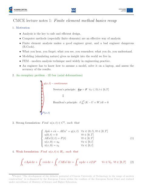
2. An exemplary problem - 1D bar (axial deformations)
q(x,t) − continuous
d
Newton’s principle:
dtp = F ∀ω ⊂ Ω,t ∈ [0,T]
⇕
Hamilton’s principle: δ ∫ T
0
(K − U + W)dt = 0
P(x,t)
3. Strong formulation: Find u(x, t) ∈ C 2 , such that
⎧
⎪⎨
⎪⎩
Aρü + c ˙u − AEu” = q(x, t) ∀x ∈ (0, l), ∀t ∈ [0, T]
u(0, t) = 0 ∀t ∈ [0, T]
AEu ′ (l, t) = P(t) ∀t ∈ [0, T]
u(x, 0) = u 0 ∀x ∈ [0, l]
˙u(x, 0) = v 0 ∀x ∈ [0, l]
(1)
4. Weak formulation: Find u(x, t) ∈ H 1 , such that
∫ l
0
vAρü dx +
∫ l
0
vc ˙u dx +
∫ l
0
v ′ AEu ′ dx =
∫ l
0
vq dx + v(l)P ∀v ∈ V 0 , ∀t ∈ [0, T] (2)
1 Project ”The development of the didactic potential of Cracow University of Technology in the range of modern
construction” is co-financed by the European Union within the confines of the European Social Fund and realized
under surveillance of Ministry of Science and Higher Education.

2
5. Finite element method
Let’s assume that ˙u = 0. Then u = u(x).
• Discretization (finite elements)
1 2 3
1 2 3 4 5 6
1
2
1
2 3
1
3
2
• Shape functions (on element 3, using local enumeration)
ˆϕ 1 (x) = (x − x 2)
(x 1 − x 2 ) , ˆϕ 2(x) = (x − x 1)
(x 2 − x 1 ) , ˆϕ 3(x) = (x − x 1 )(x − x 2 )
remarks: ˆϕ 1 (x) + ˆϕ 2 (x) = 1, ˆϕ 1 (x) + ˆϕ 2 (x) + ˆϕ 3 (x) ≠ 1
position of the third node is neither specified nor used
• Approximation of solution (over element 3)
u h (x) = α 4 ϕ 4 (x) + α 5 ϕ 5 (x) + α 6 ϕ 6 (x)
α 4 = u h (x 4 ), α 6 = u h (x 6 )
• Approximation of geometry (on element 3)
x = x 4 ˆϕ 1 (x) + x 6 ˆϕ 2 (x)
• Element stiffness matrix and load vector
K e ij = ∫ e ˆϕ′ iAE ˆϕ ′ j dx, P i = ∫ e ˆϕ iq dx
or in a matrix form (for a 2 dof element)
K e = ∫ e BT dB dx, B = [ˆϕ ′ 1 ˆϕ ′ 2], d = AE
P e = ∫ N T q dx, N = [ˆϕ
e 1 ˆϕ 2 ]
• Assembling
• Accounting for kinematic conditions
• SLE solution; Ku = P (+F); F - nodal forces for bar structures only
• Postprocessing with solution quality assessment
2 Project ”The development of the didactic potential of Cracow University of Technology in the range of modern
construction” is co-financed by the European Union within the confines of the European Social Fund and realized
under surveillance of Ministry of Science and Higher Education.