Derivation and Integration of Equations of Motion.pdf - Cal Poly

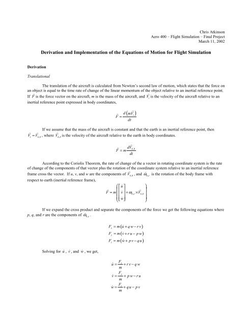
Chris Atkinson
Aero 400 – Flight Simulation – Final Project
March 11, 2002
Derivation and Implementation of the Equations of Motion for Flight Simulation
Derivation
Translational
The translation of the aircraft is calculated from Newton’s second law of motion, which states that the force on
an object is equal to the time rate of change of the linear momentum of the object relative to an inertial reference point.
If F G is the force vector on the aircraft, m is the mass of the aircraft, and V G i
is the velocity of the aircraft relative to an
inertial reference point expressed in body coordinates,
G G
V = V
i
k,
b
G
G d mV i
F =
dt
( )
If we assume that the mass of the aircraft is constant and that the earth is an inertial reference point, then
, where V G
k,
b
is the velocity of the aircraft relative to the earth in body coordinates.
G
G
F = m dt
dV k , b
According to the Coriolis Theorem, the rate of change of the a vector in rotating coordinate system is the rate
of change of the components of that vector plus the rotation of the coordinate system relative to an inertial reference
frame cross the vector. If u, v, and w are the components of V G k,
b
, and G ωb,
e
is the rotation of the body frame with
respect to earth (inertial reference frame),
⎛ ⎡u
⎤ ⎞
G ⎜
F m
⎢
v
⎥ G ⎟
= ⎜
⎢ ⎥
+ ωb, e
× Vk , b ⎟
⎜ ⎢w⎥
⎟
⎝ ⎣ ⎦ ⎠
If we expand the cross product and separate the components of the force we get the following equations where
p, q, and r are the components of G ωb,
e
.
Solving for u , v , and w , we get,
x
y
z
( )
( )
( )
F = m u + q w − r v
F = m v + r u − p w
F = m w + p v − qu
Fx
u
= + r v − q w
m
Fy
v
= + p w − r u
m
Fz
w
= + qu − p v
m

Rotational
Newton’s second law also states that the moment on an object is equal to the time rate of change of the
angular momentum of the object relative to an inertial reference frame. If T G is the moment vector on the aircraft, I, is
the moment of inertia matrix of the aircraft, and
G ωi
, is the rotation of the aircraft with respect to an inertial reference
point,
G
⎡ I
x
−I xy
−I
xz ⎤
G d ( I ω i )
⎢
T =
I I
xy
I
y
I
⎥
= yz
dt
⎢
− − ⎥
⎢ I
xz
I
yz
I ⎥
⎣
− −
z ⎦
G G
ω = ω
i
b,
k
Again, we assume that the moment of inertia matrix is constant and that earth is an inertial reference point,
,
Again, using the Coriolis Theorem,
G d
T =
G
( I ωb,
e )
dt
Carrying out the multiplication, we get,
⎡ p
⎤
G
T I
⎢
q
⎥ G G
=
⎢ ⎥
+ ω × I ω
⎢⎣ r
⎥⎦
b, e b,
e
⎡ p I
x
− q I
xy
− r
I
xz ⎤ ⎡ p I
x
− q I
xy
− r I
xz ⎤
G ⎢
T q I
y
p I
xy
r I
⎥ G ⎢
yz ω q I
b,
e y
p I
xy
r I
⎥
= − −
⎢ ⎥ + × ⎢
− −
yz ⎥
⎢r I − p I − q
I ⎥ ⎢r I − p I − q I ⎥
⎣ z xz yz ⎦ ⎣ z xz yz ⎦
Expanding the cross product and separating the components of the moment vector, L, M, and N, we get,
2 2
( r − q )
2 2
( p − r )
2 2
( q − p )
L = p I − q I − r
I + qr I − pq I + I − qr I + pr I
x xy xz z xz yz y xy
M = q I − p I − r
I − pr I + I + pq I + pr I − qr I
y xy yz z xz yz x xy
N = r I − p I − q
I + pq I + I − pr I − pq I + qr I
z xz yz y xy yz x xz
For an aircraft of standard configuration, I xy = I yz = 0, so the equations simplify to,
L = p
I − r
I + qr I − pq I − qr I
x xz z xz y
2 2
( p − r )
M = q
I − pr I + I + pr I
y z xz x
N = r
I − p
I + pq I − pq I + qr I
z xz y x xz

If we solve the rotational equations for p , q , and r , we get,
2 2
( ) ( )
L I + N I + pq I I − I I + I I + qr I I − I − I
p
=
I I
z xz x xz y xz z xz y z xz z
2
x z − I xz
2 2
( ) ( )
M + pr I − I + r − p I
q
=
I
z x xz
y
( ) ( )
N + pq I − I + p − qr I
r
=
I
x y xz
z
The three translational and three rotational equations of motion are the bases for the equations of motion in the
flight simulator.
F
m
Fy
v
= + p w − r u
m
F
m
x
u = + r v − q w
z
w = + qu − p v
2 2
( ) ( )
L I + N I + pq I I − I I + I I + qr I I − I − I
p
=
I I
z xz x xz y xz z xz y z xz z
2
x z − I xz
2 2
( ) ( )
M + pr I − I + r − p I
q
=
I
z x xz
y
( ) ( )
N + pq I − I + p − qr I
r
=
I
x y xz
z

Implementation
Translational
In the flight simulator, the forces on the aircraft is the sum of the external forces, aerodynamic forces, and
gravitational forces.
F = F + F + m g
x x ext, b x aero, b x,
b
F = F + F + m g
y y ext, b y aero, b y,
b
F = F + F + m g
z z ext , b z aero, b z,
b
Using the translational equations of motion derived above, we can solve for the acceleration of the aircraft.
F
m
Fy
v
= + p w − r u
m
F
= + −
m
x
u = + r v − q w
z
w qu p v
The acceleration of the aircraft is integrated over time with an initial velocity to get the velocity of the aircraft.
∫
∫
∫
u = u
dt + u
v = v
dt + v
0
0
w = wdt + w
The velocity of the aircraft is then converted into earth coordinates and integrated with an initial position to
get the position of the aircraft in earth coordinates.
0
⎡x
⎤ ⎡u
⎤
⎢ e
y
⎥
= C
⎢
b
v
⎥
⎢ ⎥ ⎢ ⎥
⎢⎣ z
⎥⎦ ⎢⎣ w⎥⎦
⎡cosθ cosψ sinφ sinθ cosψ − cosφ sinψ cosφ sinθ cosψ + sinφ sinψ
⎤
C =
⎢
cosθ sinψ sinφ sinθ sinψ cosφ cosψ cosφ sinθ sinψ sinφ cosψ
⎥
⎢
+ −
⎥
C = C
⎢⎣
−sinθ sinφ cosθ cosφ cosθ
⎥⎦
b e b T
e b e
∫
∫
∫
x = x
dt + x
0
y = y
dt + y
z = z
dt + z
0
0

Rotational
The moments on the aircraft in the flight simulator are the sum of the external moments and aerodynamic
moments.
L = L + L
ext
ext
ext
aero
M = M + M
N = N + N
The rotational equations of motion derived above are used to calculate the angular accelerations of the aircraft.
aero
aero
2 2
( ) ( )
L I + N I + pq I I − I I + I I + qr I I − I − I
p
=
I I
z xz x xz y xz z xz y z xz z
2
x z − I xz
2 2
( ) ( )
M + pr I − I + r − p I
q
=
I
z x xz
y
( ) ( )
N + pq I − I + p − qr I
r
=
I
x y xz
z
aircraft.
The angular accelerations are integrated with an initial angular velocity to get the angular velocity of the
∫
∫
∫
p = p
dt + p
q = q
dt + q
r = r
dt + r
0
0
0
The angular velocities are then converted into Euler axes and integrated with initial Euler angles to get the
Euler angles of the aircraft.
⎡ψ
⎤ ⎡ p⎤
⎢ ˆ ε
θ
⎥
= C
⎢
b
q
⎥
⎢ ⎥ ⎢ ⎥
⎢
⎣φ
⎥⎦ ⎢⎣ r ⎥⎦
⎡0 sinφ secθ cosφ secθ
⎤
ˆ
C ε b
=
⎢
0 cosφ
sinφ
⎥
⎢
−
⎥
⎢⎣
1 sinφ tanθ cosφ tanθ
⎥⎦
∫
∫
∫
ψ = ψ
dt + ψ
θ = θ
dt + θ
φ = φ dt + φ
0
0
0

Angle of Attack and Sideslip Angle
To calculate the angle of attack and sideslip angle of the aircraft, we must first calculate the air velocity of the
aircraft in body coordinates. The air velocity is equal to the ground velocity of the aircraft minus the wind velocity
converted into body coordinates. The acceleration of the aircraft relative to the air is calculated by taking the derivative
of the air velocity and applying the Coriolis Theorem.
G G G b
dV d ( Ce
Vatm,
e )
V = V − C V
b
T , b k , b e atm,
e
u = u − u
T
v = v − v
T
T
atm
atm
w = w − w
atm
G G
G
k , b
VT , b
= −
dt dt
u = u + q w − r v − u
− q w + r v
T atm atm atm
v = v + r u − p w − v
− r u + p w
T atm atm atm
w = w + p v − qu − w
− p v + qu
T atm atm atm
The angle of attack and sideslip angle can then be calculated from the components of the air velocity. The rate
of change of the angle of attack and sideslip angles is calculated by taking the derivatives of the angles.
−1
wT
α = tan
uT
u w
− u
w
α
=
T T T T
2 2
uT
+ wT
β = sin
−1
2 2 2
T
+
T
+
T
⎛
1 ⎜ v u u + v v + w w
β = v
cos β
⎜
−
⎜ u v w ( u + v + w
⎝
)
v
T
u v w
T T T T T T T
T
3
2 2 2 2 2 2 2
T
+
T
+
T T T T
⎞
⎟
⎟
⎟
⎠
Aerodynamic Forces
The atmospheric forces and moments on the aircraft are calculated using linear Taylor expansions and stability
derivatives. The derivatives are non-dimensional and must be dimensionalized using the airspeed, wing planform area,
span, and chord. The aerodynamic forces are assumed to be in stability axes and must be converted to body
coordinates.
2 2 2
T
=
T
+
T
+
T
V u v w
( α
L )
δ
1 2
x aero, s
= − ρ
2 T D
+
1 D
α + δe
e
F V S C C C
F V
⎛
S C C
b
p C
b
r C C
⎝
1 2
y aero, s
= ρ
2 T ⎜ y
β +
y
+
pˆ
y
+
rˆ
y
δa +
β δ y
δr
a δr
2VT
2V
T
F V
⎛
S C C C
c
C
c
q C
⎝
1 2
z aero, s
= − ρ
2 T ⎜ L
+
1 L
α +
L
α +
aˆ
L
+
α
qˆ
L
δ
δ e
e
2V
T
2V
T
⎞
⎟
⎠
⎞
⎟
⎠
F
= C F
b
aero, b s aero,
s
b
C s
⎡cosα
0 −sinα
⎤
=
⎢
0 1 0
⎥
⎢ ⎥
⎢⎣
sinα
0 cosα
⎥⎦

L V
⎛
Sb C C
b
p C
b
r C C
⎝
1 2
aero
= ρ
2 T ⎜ l
β +
l
+
pˆ
l
+
rˆ
l
δa +
β δ l
δr
a δr
2V
T
2V
T
⎛
c c
M V Sc C C C C q C
¡
⎝
1 2
aero
= ρ
2 T ⎜ m
+
1 m
α +
m
α +
aˆ
m
+
α
qˆ
m
δ
δ e
e
2V
T
2V
T
N V
⎛
Sb C C
b
p C
b
r C C
⎝
1 2
aero
= ρ
2 T ⎜ n
β +
n
+
pˆ
n
+
rˆ
n
δ
a
+
β δ n
δr
a δr
2V
T
2V
T
⎞
⎟
⎠
⎞
⎟
⎠
⎞
⎟
⎠
Load Factor (g’s)
The load factor of the aircraft is calculated by dividing the sum of the non-gravitational forces in the z
direction by the weight of the aircraft.
Fz aero, b
+ Fz ext,
b
n = −
mg
Integration
All numerical integration for the equations of motion is performed using the Adams-Bashforth-Moulton
method.
1
x =
∫
x dt → x
1 2
( 3
n
= xn−
+ x n
− x n−1
) dt
The equations of motion are written in C++ as a Simulink S-Function for use in the Cal Poly Pheagle Flight
Simulator. A previous implementation of the equations of motion was used as a template.