Developement Of An Instrument Landing Simulation ... - Cal Poly

Development of an Instrument Landing Simulationfor Cal Poly’s Flight Simulator using MATLAB/SimulinkPresented to:The Faculty and Representatives ofCalifornia Polytechnic State University, San Luis ObispoAerospace Engineering DepartmentIn Fulfillment of:Master of Science in Aerospace EngineeringSubmitted by:Robert A. Barger6/7/00

Authorization PageI grant permission for the republication of this thesis in its entity, or any of itsparts, without any further authorization by me.______________________Signature______________________Datei

Approval PageTITLE: Development of an Instrument Landing Simulationfor Cal Poly’s Flight Simulator using MATLAB/SimulinkAUTHOR: Robert A. BargerDATE: Friday, May 26 th , 2000__________________________________Dr. Daniel J. Biezad – Advisor__________________________________Signature__________________________________Dr. Jin Tso – Committee Member__________________________________Signature__________________________________Dr. Jordi Puig Suari – Committee Member__________________________________Signature__________________________________Edward Burnett – Committee Member__________________________________Signatureii

AbstractMost people learn by seeing, hearing, or feeling. Of these senses, the one thatgenerates the most productive learning is visual stimulation. Engineering students spendmost of their time calculating values for theoretical variables but never see them applied.Cal Poly’s Flight Simulation Laboratory enables students to visualize these variables andsee them in action through cockpit instruments and 3-Dimensional visuals. The primarypurpose of this thesis is to develop a simulation laboratory that can be integrated into theclassrooms and enable the students to learn the simulation in the shortest time possible.Not many schools have a flight simulator where students can design and build asimulation from beginning to end. The Cal Poly Flight Simulation Laboratory hascomputers, analog hardware, a simulator cab, software, and state-of-the art visuals thatcreate an entire set of tools, which allow students to become complete flight simulationengineers. The students learn the information that is being sent to the pilot, which givesthem a better understanding of the pilot’s point of view. Students not only learn theAeronautical Engineering side of flight simulation (developing the equations of motion),but they also learn the Computer Science and Electrical Engineering side of simulationby integrating computers with analog hardware.Future capabilities for the Cal Poly Flight Simulation Laboratory are endless.Students can develop a simulation as detailed as possible as long as new simulations areadded to the system and new hardware is upgraded to the lab. Currently the laboratoryhas only one flight simulator, but with the advent of new dynamic technology, it ispossible to add several simulators to develop a simulation arena.iii

AcknowledgementsI would like to thank Doug Hiranaka and Fritz Anderson for their initialdevelopment of this project. Fritz Anderson created the hardware integration of thesimulator cab with the software code. Doug Hiranaka developed the interface of the nonlinear,six-degree-of-freedom simulation using Matlab’s Simulink. I would like to alsothank the following people for their help on the simulator during the past few years.Aaron Munger’s knowledge on the simulator’s hardware aided in the development of theanalog section of this thesis. Jon Tonkyro provided expertise in networking and helpedwith the graphics. Edwin Casco and Paul Patangui assisted in the development of anInstrument Landing System (ILS) Simulation. Members from the Spring AERO 320helped with the engine model simulation. Jeff Nadel helped with the lab networking forthe ATL building. Dan Powell helped with moving the simulator and electricalassistance. Dr. Daniel J. Biezad’s continued efforts to make flight simulation and controlsa strong emphasis at Cal Poly, San Luis Obispo. David Lowe and the F-18 and UH-1Nsimulation groups at Manned Flight Simulator gave me experience and insight on howflight simulators should be developed. Finally, I would like to thank Linda Jarrard for hersupport during the time I invested on this project.iv

Figure 9: Stick Computer.............................................................. 102.1.6 Siblinc .............................................................................................. 11Figure 10: Siblinc.......................................................................... 112.1.7 Trace Card........................................................................................ 11Figure 11: Trace Card .................................................................. 112.2 Computer Hardware ........................................................................................ 13Figure 12: Instructor Operating Station (IOS)......................................... 132.3 Computer Software ......................................................................................... 142.3.1 Simulink and Real-Time Work shop................................................ 142.3.2 S-Functions....................................................................................... 152.3.3 C-Code ............................................................................................. 152.3.4 TCP-IP/UDP..................................................................................... 152.3.5 OpenGVS ......................................................................................... 162.3.6 D/A A/D Channel............................................................................. 172.4 Analog Output................................................................................................. 19Figure 13: Analog Output Schematic........................................................ 192.4.1 Stick and Rudder Signals ................................................................. 202.4.2 Instrument and Console Signals....................................................... 20Figure 14: IJ1 & IJ2 ..................................................................... 20Figure 15: Instrument Connections .............................................. 202.5 Visual Output .................................................................................................. 212.5.1 Front Cockpit Visuals....................................................................... 21Figure 16: Front Cockpit Visuals ................................................. 21vi

Figure 17: Front Cockpit IOS....................................................... 222.5.2 Rear Cockpit Visuals........................................................................ 22Figure 18: Rear Cockpit Visuals................................................... 22Figure 19: Rear Cockpit IOS ........................................................ 223. Simulation Operations Procedures............................................................................ 243.1 PhEagle Operations Manual............................................................................ 243.2 PhEagle Virtual Library .................................................................................. 243.2.1 Models.............................................................................................. 253.2.1.1 Stick Model ....................................................................... 25Figure 20: Stick Model...................................................... 253.2.1.2 Engine Model .................................................................... 26Figure 21: Engine Model .................................................. 263.2.1.3 Standard Atmosphere Model............................................. 27Figure 22: Standard Atmosphere Model........................... 273.2.1.4 SixDOF Model .................................................................. 27Figure 23: SixDOF............................................................ 273.2.1.5 Instrument Model .............................................................. 28Figure 24: Instrument Model ............................................ 283.2.1.6 Graphics Model................................................................. 28Figure 25: Graphics Model............................................... 283.2.1.7 ILS Model ......................................................................... 29Figure 26: ILS Model........................................................ 293.2.2 Tutorials ........................................................................................... 29vii

3.2.2.1 Times Two Tutorial........................................................... 303.2.2.2 Speed of Sound Tutorial.................................................... 303.2.3 Documentation ................................................................................. 304. Simulation Development............................................................................................. 314.1 Graphics .......................................................................................................... 31Figure 27: Pilot Verification..................................................................... 314.1.1 Terrain Database .............................................................................. 32Figure 28: Korean Database ........................................................ 32Figure 29: Monterey Database..................................................... 324.1.2 Instrument Landing Simulation........................................................ 32Figure 30: Takeoff / Landing Scenario......................................... 33Figure 31: CDI & ILS ................................................................... 344.2 Rear Cockpit.................................................................................................... 344.3 Heads-Up Display ........................................................................................... 354.4 Combat Simulator ........................................................................................... 354.5 Combat Simulation Arena............................................................................... 354.6 Projectors......................................................................................................... 36Figure 32: Projector Setup ....................................................................... 36Figure 33: Three-Projector Display ......................................................... 374.7 Calibration....................................................................................................... 374.7.1 Instrument Calibration...................................................................... 37Table 1: Instrument Checklist ....................................................... 38viii

4.7.2 Throttle Calibration.......................................................................... 38Figure 34: Initial Throttle Readings ............................................. 39Figure 35: Throttle Analog Output ............................................... 40Figure 36: Corrected Throttle Output .......................................... 404.8 Graphical User Interface (GUI)....................................................................... 415. Simulator Implementation ......................................................................................... 425.1 Stability Derivatives........................................................................................ 425.2 Flight Control System Design......................................................................... 43Figure 37: Glide Slope Simulation............................................................ 435.3 VFR & IFR Landing Simulation..................................................................... 435.4 Guidance & Control ........................................................................................ 446. Conclusion.................................................................................................................... 45ix

1. Introduction:Flight simulations take years to develop. In industry, a team of 50 or moreengineers work on the simulation for a simulator, which allows it to become as real aspossible. Industry simulation labs contain several networked simulators to create asimulation arena. The goal of Cal Poly’s Flight Simulation Laboratory is to develop amulti-role simulator within a simulation arena. This will enable the simulator to modelany aircraft and will allow several aircraft to fly within the same three-dimensionalworld. To accomplish this goal, years must be invested to develop the code to run thesimulation.Simulations are quite complex. Flight simulation engineers must not only knowbasic aircraft dynamics and controls, but they must also understand programming,networking knowledge, hardware, standards, etc. This thesis develops a baseline forachieving the simulation arena goal and sets a standard for training a flight simulationengineer.1.1 Computers and HardwareThe flight simulator consists of the Pheagle cab and two analog computers, whichcomplete the link between the digital computers. The simulation is affordable because ituses four Pentium 166 computers and common software. This also allows thecommunication from the analog realm to be accessed from the digital realm with the useof A/D and D/A cards. Since the digital realm is split into multiple computers, thecomputing power is endless. As processors and graphic cards become faster and better,1

the simulation is transportable to any platform. More digital and analog hardware can beimplemented in the simulation allowing further research into futuristic cockpit displays orimbedded avionics. Due to the networking capability of the simulation, simulators can beadded as long as there is enough bandwidth. Desktop simulators or other analogsimulators can be added to the simulation to develop a simulation arena.1.2 SoftwareThe simulation integrates C-code with Matlab’s Simulink S-Function AppliedProgrammer’s Interface (API). Simulink’s Graphical User Interface (GUI) allows theuser to see the variables flow through the simulation. At any time, the user can monitor orgraphically display one of the variables and plot it as a function of time. This is far betterthan debugging in most common compilers since Simulink allows the programmer to seethe variables in real-time. Simulink also allows the simulation to be broken down intosubsystems and individual simulation models. These models can be individually tested oradded to a completely different simulation.Simulink’s S-Function API allows any C-Code to be integrated into thesimulation. This allows the implementation of other API’s into the simulation. OpenGVSis another API that uses OpenGL code to generate a Realtime Scene Management forThree-Dimensional Visuals. OpenGVS has specific functions that enable the threedimensionalenvironment to be changed such as camera position, lighting, and visibility.1.3 PhEagle Archive2

The simulation laboratory needs to continue its ongoing development. This meansthat running and developing the simulator needs to become easy to learn in the shortesttime possible. The development of the PhEagle Virtual Library enables senior projects,thesis work, research, and simulation models to be well documented, stored, and easilyaccessible, so students can begin where the last student finished. This will allow thesimulator’s development to be ongoing and keep up with industry. Included are tutorialsand demos, which teach the students how to create a simulation and learn differentaspects of the simulator. The Pheagle Operations Manual thoroughly describes how torun the simulator and how to test and calibrate any of the hardware, instruments, orsimulations.1.4 Research ObjectivesThe initial goal was to develop a visual systemfor the simulator that led to the development of anInstrument Landing System (ILS) Simulation. Beforethis could happen, the simulator had to be moved intothe new Northrop Grumman Aerospace SystemLaboratory in the Advanced Technology Laboratories(ATL) building at Cal Poly, San Luis Obispo, shownin Figure 1. This led to the development of the newFigure 1:Advanced Technologies Laboratories(ATL)simulation laboratory.In order for the ILS simulation to work, an adequate engine model had to bedeveloped. Also the ILS and CDI instruments were not working at the time of3

development. These models had to be generated, calibrated, and tested. Once these werecompleted, the graphics had to be implemented into the simulation complete with anairport and terrain database. Once completed, the simulation starts the aircraft at adistance from the airport where the pilot uses the instruments along with the visuals toland the aircraft at the airport.1.5 Continuing ResearchThe next step is to integrate multiple aircraft into the simulation arena. Thesimulator cab is a two-seater, which allows the addition of another cockpit. The rearcockpit is entirely digital complete with a flat screen display, a gaming joystick, throttle,and rudder pedals. This will enable the simulator to have “dog fighting” capability. Sincethe rear cockpit is entirely digital, it can be copied to create another desktop simulator,which can be added to the simulation to create a flight simulation arena.4

2 Simulation Flow:The PhEagle Flight Simulator is quite complex due to the interaction between thedigital and analog signals; therefore, it is important to understand the signal flow of thesimulation. This enables the operator to be able to trace a signal to see if it is getting toand from the simulator cab. Figure 2 gives a simplified description of the input andoutput signals to and from the cab, the analog computers, and the digital computers. Theyellow arrows represent inputs to the I/O computer, Spiegel, and the green arrowsrepresent the outputs. In general the cab sends stick and rudder inputs to the stickcomputer, and throttle inputs are sent to Siblinc. The signal then gets mapped to A/Dcards located in Spiegel through the trace card. Spiegel then computes the equations ofmotion to generate the states of the aircraft. The position and orientation is sent to each ofthe three visual computers, Eagle, Phantom, and Pheagle, which display the center, left,Instruments & LightsPhantom(Left View)PhEagle CABThrottle InputsStick & RudderInputsSiblincTraceCardSpiegel(EOM)ETHERNETEagle(Center View)PheagleStick & Rudder ForcesStickComputerFigure 2: Simulation Flow Schematic(Right View)5

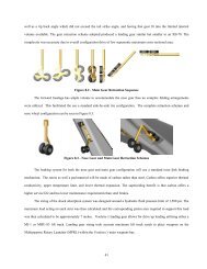
and right views respectively.Spiegel also sends out analog signals to the cab. Instrument settings and lights aresent through Spiegel to Siblinc then to the cockpit. Stick and Rudder forces are sent to thestick computer and then to the stick and rudder to generate force-feed back. Each of thesesections will be broken down to give a more detailed description of the signal flow.2.1 Analog InputThe incoming analog signal to Spiegel reads the signals from the stick, rudder,and throttle and the left and right console panels. Figure 3 shows a schematic of theanalog input from the stick, rudder, throttle, and consoles to the I/O computer, Spiegel.Stick & RudderMotorsTraceCardStickRudderBottom TorqueMotor AssemblyStick ComputerCockpit JunctionBox (CJB)SpiegelThrottle CardTraceCardThrottlesLeft ConsoleCardandJ – ConnectorsLeft ConsoleRight ConsoleRight ConsoleCardFigure 3: Analog Input SchematicSiblinc6

The analog inputs are broken down into control inputs or switches. Control inputsinclude the stick, rudder, and throttle inputs. Switches include any of the switcheslocated on the consoles, the stick, or the throttle. The stick and rudder inputs send signalsto both the Siblinc and the Stick Computer. The throttle is located on the left console andis connected to the left console card. Both console cards connect to the Cockpit JunctionBox (CJB) located beneath the simulator. Any signals connected to the CJB get sent toSiblinc.Control inputs send voltage signals to Siblinc and/or the Stick Computer based onthe control device. These inputs then get scaled to a range of +/- 5 volts. This voltage isthen sent to the trace card where the signals are broken down to the desired pinarrangement for the corresponding A/D card, located within Spiegel.2.1.1 StickStick inputs can be the stick position,velocity, and stick trim settings as well as thebuttons located on the stick such as the triggerand the hat switch. Originally the simulator cabwas an F-4 Phantom simulator. The stick is anF-15 Eagle stick, shown in Figure 4, which wasadded to the simulator for handling qualitiesresearch at NASA Dryden. Hence, with thecombination of the two, the simulator receivedFigure 4: F-15 Stickits name PhEagle.7

The stick is connected to the sticktorque motor located below the simulatorcab, shown in Figure 5. A voltage is sentto the motor to enable it to read the stickposition and output stick forces. The stickacts like a potentiometer, and based onthe stick position, it will send a voltage toFigure 5: Stick Motorthe Stick Computer and Siblinc. This voltage will then be scaled down based on thepotentiometer settings. The Spiegel computer requires a voltage range of +/- 5 volts. Thevoltage input is then ran through the trace card to the A/D cards located within Spiegel.The input is then read in through the compiled C-Code and Simulink to generate anominal input range of +/- 1.0 in decimal form and ready to be run through thesimulation.2.1.2 RudderRudder inputs are very similar to the stickinputs. The rudder inputs are the rudder position,velocity, and the trim settings. Just like the stick,the rudder has a torque motor, shown in Figure 6.This too acts like a potentiometer and sends avoltage based on the rudder position to the StickComputer and Siblinc. This voltage will then beFigure 6: Rudder Torque Motor8

scaled down just like the stick to a range of +/- 5 volts and generate a digital value of +/-1.0.2.1.3 ThrottlesThe throttle input is the right and left throttlesetting as well as the buttons located on thethrottles. Figure 7 shows the two-engine throttleconfiguration in the simulator. If the aircraft hastwo engines, each throttle can be set individuallyto control the output of each engine. If theFigure 7: Throttlesaircraft has only one engine, the thrust is divided in half by each engine setting. Thethrottle generates an input of a nominal percentage from 0 to 1. Within the throttle regionthere are four stops: OFF, IDLE, MIL, and MAX. OFF is at 0% thrust, IDLE is at 10 %,MIL is at 62 %, and MAX is at 100 %. If the engine being modeled is a jet equipped withan afterburner, the afterburner range is from MIL to MAX. In order to engage theafterburners, the grasps underneath the throttle must be pulled. Additional buttons on thethrottle are flap settings, rudder trim, and buttons and switches that could be used forspeed brakes, communication buttons, etc. All throttle inputs get fed to the left consolecard.2.1.4 ConsolesThe right and left console each have an independent card to read in the input such aspitch, roll, and yaw control augmentation switches, stick force on/off switches, and more.9

Currently, the only console card integratedinto the simulation is the left console card,shown in Figure 8. There are additionalcards for both the left and right console. Toreceive inputs from the right console, theright console card would have to bemounted and connected into the simulator.Figure 8: Left Console Card2.1.5 Stick ComputerThe stick computer controls the inputs andoutputs to and from the stick and ruddermotors. The most important feature of thestick computer is that it can generate excellentstick and rudder feel since its main purposewas for handling qualities research. The stickcomputer is broken into three sections: pitch,roll, and yaw. The three axial forces can bemodified for force gradients, damping,breakout, and stop locations. Figure 9 showsFigure 9: Stick Computerthe stick computer with the different potentiometers located on the front panels. Otherimportant features on the analog computer are trim settings, surface position, and amountof force generated by the motors. Each motor has the capability of generating 50 poundsof force.10

2.1.6 SiblincSiblinc is the other analog computer thatcontrols the channels being sent to and from thecab. 1 Figure 10 shows Siblinc with its manychannels located on the front panel. Each channelhas three potentiometers. These set the NULL,BIAS, and SCALE for each channel. The middlesection of Siblinc contains a patch voltmeter thatallows each signal to be monitor coming intoSiblinc and going out of Siblinc. The bottomFigure 10: Siblincsection contains additional channels for switches and lights. The main purpose of Siblincis to modify the signal going to and from the cab so that the output or input voltage of thecab is scaled to +/- 5 volts for the I/O computer, Spiegel.2.1.7 Trace CardThe trace card is the key to break the gap fromthe analog realm to the digital realm. 2 Figure 11shows the green trace card located on the back ofcabinet of the instructor operating station. This cardallows each channel to be split up into either aninput or and output. If the signal is an input signal, itgoes to one of the A/D PC lab cards. If the signal isFigure 11: Trace Card11

an output, it is sent from either the 16 bit D/A card, or the 12 bit D/A card. The tracecard receives three connectors from Siblinc. An additional connector is also sent fromSiblinc, however, the channels within this connector are not known. To add thesechannels to the simulation another trace card would need to be added as well as someadditional A/D and D/A cards. Luckily, additional cards are located within the hardwarecabinet.12

2.2 Computer HardwareThe computers integrated into the simulationare four Pentium 166 computers. Figure 12 shows theInstructor Operating Station (IOS) where eachcomputer is mounted within the cabinet. Eachcomputer serves a distinct purpose. This allows thesimulation to be run in real-time since each computeris designated for a specific task. The I/O Computercontains four data acquisition cards: a 16 and a 12 bitDigital-to-Analog (D/A) card, a 12 bit Analog-to-Figure 12: InstructorOperating Station (IOS)Digital (A/D) card, and a 48 bit digital input/output card. The I/O computer handles theanalog inputs and outputs to the simulation as well as computing the Equations OfMotion (EOM) to solve for the aircraft’s position, orientation, and state, which are sent tothe two analog computers as well as the three visual computers.Each of the four digital computers contains a network card and can communicatethrough a network hub, which creates a Local Area Network (LAN), or Intranet. TheI/O computer acts as a server and sends the aircraft’s position, orientation, and state, toeach of the visual computers, which act as clients. Each visual computer is equipped withan Obsidian 2 Quantum 3D graphics card, which is basically a modified 3Dfx Voodoo 2card. Each of these cards is set to run the glide hardware. Additional hardware is soundcards located within Eagle and Pheagle, and additional data acquisition cards in Phantom.13

2.3 Computer SoftwareThe four computers each run Windows 95 as their operating system. This allowsany windows applications to be implemented in the simulation. Older simulationlaboratories use VAX or VMS machines to run the simulation. With the advent of faster,low cost PC’s, the Windows platform allows students to work in a familiar environment.This also allows the portability of adding new software to the simulation.Currently, the computers are equipped with MATLAB, Simulink, and the RealTime Workshop to run the simulation. 3 These computers use Visual C++ 6.0 to compilethe simulation code, and the visual software is generated using OpenGVS.2.3.1 Simulink and the Real-Time WorkshopThe PhEagle simulation runs in Simulink by MATLAB. If the simulation was leftentirely as code, the programmer would be lost not knowing which variables were beingsent, which variable names are being used, and the file order. Simulink allows thisprocess to become simple. Simulink allows the students to visually map the variables asthe simulation computes them. Simulink also allows the users to easily grab a variableand monitor it or link it to a subsystem within the simulation. Variable names don’t haveto match for the code to run. The file order is easy to see as the programmer can followthe flow of the simulation and visually see the order that files get called within thesimulation.The Real-Time Workshop allows the simulation time-differential to be changed. 4This allows a more accurate integration to keep the simulation running in real time. This14

also allows the entire simulation to be compiled into one executable. Programs can begenerated, distributed, then tested in the classrooms, or students can use them at home.2.3.2 S-FunctionsThe Real-Time Workshop in conjunction with Simulink requires the code to bewritten in a special S-Function format. 5 This allows different sections of the code to berun at different times during the simulation. 6 For instance, the S-Function requires thecode to have a start, initialize, sample time, output, and termination sections. The startsection is only called the first time the simulation runs. The initialize section initializesthe size of the input and output arrays. The sample time section determines the timedifferential for the simulation. The output section computes the output variables. Thetermination section allows conditions to be set to terminate the simulation. Various othersections can be added to make the code behave how and when the programmer wants itto.2.3.3 C-CodeThe C-Code for the simulation is written in the S-Function format. 7 If the code isin the correct format, the compiler will generate a dynamic linked library (dll). This iscompiled C-Code much like an executable. Simulink searches for this dll based on the S-Function name that was assigned to it. To generate the dll, the compiler must be set upcorrectly so Matlab knows where to find it. The code cannot be written in C++, it mustonly be written in C. The entire code for the simulation was written by students.15

2.3.4 TCP-IP/UDPSince the computers are networked together, code had to be written tocommunicate between the two. The goal was to have the I/O computer, Spiegel, computethe aircraft’s position and orientation and send that information to the other three visualcomputers to generate the graphics. A sample program was written in C++ for a UNIXplatform to test the functionality of sending information across the Internet. 8 One side ofthe program acted as the server and the other program played the client. This programthen had to be modified to work under Windows using winsockets. Once the programproved to work, it had to be modified again to work using UDP. UDP is similar to TCPexcept that it allows the communication to be connectionless. Once the program wasworking, the code had to be converted to C then added to a test bed simulation withinSimulink. The program was tested, and it worked perfectly with little lag in the framerate. The final step was to have the test bed simulation work with the graphics since thecommunication barrier had been breached; the next step was to have the model work withthe graphics.2.3.5 OpenGVSOpenGVS offers excellent 3-D rendering scene software that is already set up forflight simulation. 9 OpenGVS already has imbedded functions that allow terrain databases,camera views, vehicles, lighting, etc. to be simply added to the simulation. Includedwithin OpenGVS are demo programs that give a programmer an idea of how to createvisuals. The demos include a Heads-Up-Display (HUD) demo that has an aircraft flythrough a database of Korea in a Mig-29 armed with missiles. Other demos include a16

tank demo with different helicopters and tanks within the same battlefield, and aMonterey demo that starts the aircraft in final approach. The demos also included amaster/slave program that would be perfect as a baseline for networking visuals. Theserver code was created to send the aircraft’s position and orientation. The client codewas modified to work as the slave within the OpenGVS environment. Once completed,the aircraft simulation ran in Matlab’s Simulink to compute the aircraft’s position andorientation. It was then sent from Spiegel to the Graphic computers via the server code,where a client on each computer received the aircraft’s information and displayed it onthe screen. The terrain database can be chosen by an initialization file as to whether thedatabase is to be Monterey or Korea. The Korean database contains snowy mountainswith deep canyons, and the Monterey database has an airport with runway lights andglide slope markers. The objective is to develop an instrument landing simulation usingthe Monterey database with the airport and integrate an Instrument Landing System(ILS) model.2.3.6 D/A A/D ChannelBesides the visual output, analog output had to be sent to the cab to drive theinstruments. To do this the D/A and A/D cards had to be integrated into the simulation 10 .This was done by developing a class for each card and creating a channel within the classfor each input or output. Each channel is set and initialized with a channel number andthe max input/output range.17

2.4 Analog OutputThe simulation sends the outputs to the instruments with the use of an instrumentmodel. This model receives the instrument values and sends them to the cab. The valuesare set to a D/A channel on the D/A card. The card sends the signal on a range of +/- 5volts to the Trace Card. The trace card then connects to the Siblinc and the StickComputer. The +/-5 volt signal gets modified for the analog target within the cab. Figure13 shows the analog output schematic.Stick & RudderMotorsTraceCardStickRudderBottom TorqueMotor AssemblyStick ComputerCockpit JunctionBox (CJB)SpiegelTraceCardL & R ConsoleRight & LeftConsole CardsandJ – ConnectorsInstrumentsInstrumentMotherboardFigure 13: Analog Output SchematicSiblinc18

2.4.1 Stick and Rudder SignalsThe stick and rudder can receive stick force commands from the simulation basedon the amount of g’s being generated by the aircraft maneuvers. This force is sent to thestick computer, which sends the signal to the stick and rudder torque motors to generatethe force. These forces can generate up to 50 pounds of force.2.4.2 Instrument and Console SignalsFrom Siblinc, several connectors split the signalfrom Siblinc to the instruments and consoles. Initially, thesignal gets sent to the cockpit junction box (CJB) where itthen gets sent to the instrument panel motherboardassembly. Two connectors attach the signals to themotherboard, these are known as IJ1 & IJ2. Figure14shows these connectors mounted to the motherboard. Thesignal finally reaches its destination target by a connectionto one of the instruments from the motherboard.Figure 14: IJ1 &IJ2Figure 15 shows the back of theinstruments with their connections linking them tothe motherboard assembly. A tag on eachinstrument describes the channel number of theinstrument. This is the same channel as on Siblinc.Figure 15: Instrument Connections19

This channel also is etched into the motherboard. The Model II Cockpit, Book IV 11describes the electrical connections in detail with schematics and tables for each wiringconnection.2.5 Visual OutputThe visual output is split up into two sections, the front cockpit visuals and therear cockpit visuals. Each displays the pilot’s visuals and the Instructor Operating Station(IOS) visuals.2.5.1 Front Cockpit VisualsThe Spiegel computer also sends information about the aircraft to the visualcomputers. Figure 16 shows the front cockpitvisuals. The visuals are setup to generate threeviews. Eagle is designated as the center visualcomputer. Eagle will display the center view aswell as the HUD. Phantom and Pheagle willdisplay the left and right views respectively.Figure 16: Front Cockpit VisualsThe visuals can be either a Monterey database with an airport, or a Korean database withmountains.The pilot and the IOS have a set of visuals. Figure 17 shows the IOS visuals. TheIOS visuals are the same as the pilot’s visuals. This allows the operator to see where theaircraft is flying and still be able to monitor the state of the aircraft within the Simulinksimulation window. Also the operator can generate charts in real time or use any other20

tools that Simulink has to offer without stopping thesimulation. This allows data collection to be mucheasier and more robust. Operators can sendcommands to the pilot to get the data that they want.The IOS visuals also serve as a desktop simulator sooperators can fly and monitor the simulation bythemselves. This allows the operator to perform runFigure 17: Front Cockpit IOStime debugging without the help of others.2.5.1 Rear Cockpit VisualsThe rear cockpit simulation is similar to thefront cockpit, except that a single machine runs theback seat. The computer calculates the equations ofmotion, and displays the graphics. The rear cockpitis entirely separate from the front cockpit except forFigure 18: Rear Cockpit Visualsan Ethernet link. Figure 18 shows the back seat visual setup. A 15-inch flat screenmonitor is mounted in the back seat since a regular monitor would not fit.Similar to the front cockpit, the rear cockpithas an IOS. This serves the same purpose as the frontseat. Figure 19 Shows the IOS visuals for the rearcockpit. The increased visuals of all stations allowtwo pilots and two or more operators to monitor theaircraft’s states and the pilot’s maneuvers.Figure 19: Rear Cockpit IOS21

3. Simulation Operations Procedures:The hardest task for students working on this simulator is trying to understandhow it works. Due to its initial development there are little resources that explain how thesimulator works. In order for the learning curve to decrease, adequate documentation andresources need to be made available for the next student working on this project. ThePhEagle Operations Manual, and the PhEagle Virtual Library contain descriptions andprocedures of how to run the simulator, where to store back-up files, model descriptions,tutorials, and documentation. Each student working on the simulator will update thePhEagle Operations Manual, and the PhEagle Virtual Library.3.1 PhEagle Operations ManualThe PhEagle Operations Manual contains operations and procedures of how torun the simulator. 12 Also included are references of student work such as previousoperation manuals, student senior projects, and theses. Software, hardware, and APIimplementation are included such as Matlab GUI documentation, TCP/IP and UDPdocumentation, A/D and D/A card information. Most importantly, the source code isprinted out and located in its appropriate section describing the model.3.2 PhEagle Virtual LibraryThe PhEagle Virtual Library is much like the PhEagle Operations Manual exceptthat it is Web based. This allows a tree structure library to store documentation, code, andany other pertinent information into subsequent directories. Within the library is a22

description of each model, the corresponding code, model file, executable, anddocumentation. Also included are tutorials in HTML format. This describes a step by stepformat on how to compile code, generate models, and repeat any process that has beendone before. The last aspect of the PhEagle Virtual Library is its documentation database.This will include any thesis work, senior projects, student work, or pertinent information.3.2.1 ModelsWithin the PhEagle Virtual Library are model sections describing each model indetail. Included in each section are the Simulink model, source code, executable (dll) andany documentation. Any updates to the source code or models is to be updated to thedirectory for that model so that all models and code is current. The following are themodels entered so far in the simulation.3.2.1.1 Stick ModelThe stick model in Figure 20 reads the inputsfrom the stick, rudder, and throttles. The input is ona range of +/-5 volts and outputs +/- 1.0 in digitalform to be run in Simulink for the stick and rudderpedals. For the throttle inputs the output is inpercent of maximum thrust. This will base thethrottle setting from 0 to 1.Figure 20: Stick Model23

3.2.1.2 Engine ModelThe engine model in Figure 21 computes the thrust generated by the aircraft’sengine(s) based on the throttle setting, altitude, and static seal level thrust. 13The enginecan either be a propeller, turboprop, high by-pass ratio engine, or jet engine withafterburner or without. 14Other necessary inputs are left and right engine fuel capacity,propeller efficiency (if a propeller driven engine), TSFC, and afterburner TSFC. It thencomputes the thrust generated based on these inputs and calculates the engine RPM,temperature, fuel flow, and nozzle position.Figure 21: Engine Model24

3.2.1.3 Standard Atmosphere ModelThe Standard Atmosphere Modelis shown in Figure 22. This modelcomputes the speed of sound, density,pressure, and temperature, based onaltitude. This model also takes intoaccount the different altitude regimes thatthe aircraft is flying in and applies theFigure 22: Standard Atmosphere Modelappropriate equations.3.2.1.4 SixDOF ModelThis model computes theaircraft’s position and orientationalong with velocity, angular rates,angle of attack, sideslip, andtranslational accelerations. TheSixDOF model in Figure 23 treatsthe aircraft like a point mass. Itconverts the forces, moments,Figure 23: SixDOF Modeland control inputs generated by the aircraft to compute the above states. The term sixdegrees of freedom refers to the translational and rotational positions: X, Y, Z, and Psi,Theta, Phi. The model also reads in a Standard Aircraft Data (SAD) file, which containsthe aircraft’s stability derivatives and initial conditions.25

3.2.1.5 Instrument ModelThe instrument model in Figure 24receives the inputs from the SixDOF model. Thismodel initializes the instruments and sets therange of the instruments. The model then sendsthe values to the D/A cards, which convert it to arange of +/- 5 volts. This communication is donethrough the use of the DA Channel class. This isan excellent model for testing and calibrating theinstruments and channels.Figure 24: Instrument Model3.2.1.6 Graphics ModelThe graphics model receives the position androtation from the SixDOF model as well. It sends theinformation over the Ethernet to the three graphicscomputers using UDP. The model waits for the graphicsto initialize before it starts the simulation. It also does aconversion from aircraft axis to world axis. Figure 25shows the graphics model with the three outgoingsignals to each computer that send the aircraft’s positionFigure 25: Graphics Modeland orientation as well as whether to keep the graphics running. On the client side,26

different scenarios can be chosen, such as an instrument landing simulation to the Salinasairport in Monterey, or a Korean database filled with mountains and canyons to flythrough.3.2.1.7 ILS ModelThe ILS model in Figure 26simulates an ILS transmitter located at theend of the runway. 15 The model receivesthe aircraft’s position and calculates thedeviation off glide-slope and runwaycenterline based on the airport’s locationand heading. It then displays the angledeviations on the CDI and ILSFigure 26: ILS Modelinstruments.3.2.2 TutorialsTutorials allow students to learn certain skills required to run the simulator.Students learn how to generate code, models, and more within the tutorials. Each time astudent creates something new, the student will create a tutorial so others will learn thesame. For instance, if a student learns how to create a GUI, the student will create a GUItutorial so others will learn as well.27

3.2.2.1 Times Two TutorialThis is a simple tutorial that teaches the students how to compile code in Matlab.Although this is a simple model, since it computes the input by two, the code is quitecomplex. To do this simple model will require two pages of code.3.2.2.2 Speed of Sound TutorialThis is a more complex tutorial where the student has to create the code andmodel from scratch. Students here learn the basic S-Function format. The model receivesthe gamma, gas constant, temperature, and velocity, and computes the speed of sound andMach number.3.2.3 DocumentationAny documentation written for the simulator or that pertains to the simulator is tobe stored in the documentation directory. This primarily includes student work such astheses, senior projects, class or project work, etc. Additional documentation are helpfulreferences that pertain to the simulator development such as military standards, FAAguidelines, software documentation that pertains to Matlab, Simulink, OpenGVS,TCP/IP, UDP, etc.28

4. Simulation Development:The prior sections described how the PhEagle Simulator signals flowed and howto run and maintain the simulator as well as the lab. The next section describes thepotential of Cal Poly’s PhEagle Flight Simulator.4.1 GraphicsThe main emphasis of this thesis was togenerate graphics for the simulator. Determining theaccuracy of the aircraft model would be harderwithout graphics. Although the aircraft model islinear, the non-linear SixDOF model did an excellentjob mimicking the flight characteristics of the actualFigure 27: Pilot Verificationaircraft. Responses such as short period and phugoid oscillations as well as dutch rollmovements were evident in the model. These oscillations would occur in the actualaircraft as well. Responses to the control inputs were correct. High gain control inputswould generate a Pilot Induced Oscillation (PIO) that would cause loss of the aircraft.Several pilots flew in the simulator and agreed that the aircraft model behaved like anactual aircraft, such as the pilot in Figure 27. Overall the graphics proved that the modelis correct.29

4.1.1 Terrain DatabaseFurther development of the graphics lead to the ease of the capability ofOpenGVS. Different terrain models could be chosen to allow the pilot to fly in a Koreandatabase, shown in Figure 28, filled with mountains, or a Monterey Database equippedwith an airport, shown in Figure 29. Additional terrain databases can be added to thesimulation as long as they are in the correct format.Figure 28: Korean DatabaseFigure 29: Monterey Database4.1.2. Instrument Landing SimulationThe objective of this thesis was to develop an Instrument Landing Simulationcomplete with an airport and an ILS simulation. To make the OpenGVS databasecompatible with our simulation, a coordinate transformation had to be performed. TheOpenGVS world axis were –Z, Y, X in relation to the aircraft axis X, Y, Z. A simplemodification generated the correct output to make the two worlds compatible. Finally, thebridge between OpenGVS and Simulink had been crossed.The Instrument Landing Simulation forces the student pilot to become familiarwith the ILS. Figure 30 shows a typical takeoff / landing scenario for a student pilot’straining mission. The aircraft can either start two miles away from the airport on the30

downward approach of the runway or on the airport’s taxiway. If the aircraft starts at theairport, the pilot will takeoff and climb to an altitude of 1,000 feet heading North. Thepilot will then proceed to enter the landing pattern as they turn South.Turn to Intercept Landing PatternTakeoffRunway ApproachLandFigure 30: Takeoff / Landing ScenarioThe pilot needs to align the aircraft with the centerline of the runway using theCourse Directional Indicator (CDI) and Instrument Landing System (ILS) shown inFigure 31. The CDI shows a range of +/- 10 degrees off centerline. Once the pilot centersin on the runway within 2.5 degrees, the ILS begins to move across the instrument31

showing the pilot where he needs to position the aircraft to keep the plane centered downthe runway. Once the plane has acquired the same heading as the runway, the pilot mustadjust the plane’s glide-slope to –2.5 degrees. The pilotmust then maintain the ILS fixed on the centerline and theglide-slope in order to make a nice smooth landing.Implementation of the ILS simulation proved that theILS model was accurate since the ILS led the pilot directlyFigure 31: CDI & ILSdown the center of the runway to a smooth landing. This simulation can now beimplemented into the classrooms and students can learn how to takeoff, fly a pattern, thenland using the ILS.4.2 Rear CockpitCompletion of the baseline for the front cockpit gives rise to the addition of a rearcockpit. PhEagle is already equipped with a back seat for a navigator. The back seat wasmodified to enable the rear cockpit to be either a navigator or a pilot of a differentaircraft. Since the rear cockpit does not have an analog stick, like the front cockpit, theinput is purely digital with the use of a gaming stick, rudder, and throttle. This allows thesimulation to be entirely digital and run on one machine. Once the baseline simulation iscopied and created from the front cockpit to the rear, the only difference will be toreplace the analog input with the digital inputs from the joysticks. However, since therear cockpit has no instruments, a HUD must be generated to display the aircraft’s statesto the pilot.32

4.3 Heads-Up DisplayOpenGVS already has a demo model that creates a Heads-Up Display (HUD).Implementing this demo into the simulation will allow the aircraft’s states to be displayedon the center view for both the front and rear cockpits. The model already computes thestates needed, so all that needs to be done is to integrate the HUD into the simulation.This can be done by sending a struct containing the aircraft states across the Ethernet tothe center computer.4.4 Combat SimulatorCombat simulators require at least two or more vehicles. With the completion ofthe rear cockpit baseline with a HUD, both simulations are ready for “dog fighting”.Another model within OpenGVS uses a generic missile simulation that allows a missileto be fired when a key is pressed. Implementing this model into the simulation will allowthe simulation to be “dog fight” capable. OpenGVS already has the demos set up to allowthe number of vehicles to change. Changing this variable to two allows the aircraft to flywithin the same three-dimensional world and see each other.4.5 Combat Simulation ArenaA combat simulation arena is when more than two aircraft are fighting againsteach other in the same world. Since the rear cockpit is entirely digital, adding anotherdesktop simulator to the simulation can be accomplished by repeating what was done forthe rear cockpit. This allows not only combat scenarios but also formation flying.As many simulators can be added to the system as long as there is adequate bandwidth.33

4.6 ProjectorsThe Visuals for the PhEagle flight simulator have been proven to work for allthree views. The next step is to determine what type of visual system to use. The choicesare either monitors or projectors. Projector screens can be aligned to offer a wider field ofview and give the pilot a better sense of flying. Figure 32 gives an example of how to setup the projectors with the use of a screen. 16Figure 32: Projector SetupA projector setup was tested to see how the simulator would look with a threeprojectorsystem. Figure 33 shows the projector displays of the Korean database.This was far better than having the three monitors display the views. The 120 O field ofview gave the pilot a better sense of flying. The projectors were situated so that each ofthe views would blend into the other. When the monitors were used, the pilot’s visualdisplay would consist of breaks causing discontinuity in the graphics. In order to34Figure 33: Three-Projector Display

implement the projector system into the simulator, three projectors must be purchased.The best projectors are projectors designed for flight simulators that allow the picture tobe diffused at a close distance. In order to implement the projectors, a screen needs to bebuilt with concavity and at an arc to encompass the pilot’s peripheral vision.4.7 CalibrationOriginally the simulator was calibrated to insure that all the instruments weredisplaying the correct information to the pilot. However, when the simulator was moved,most of these instruments were no longer calibrated. Also, the throttle was notfunctioning. In order to develop an engine model, the throttles needed to be calibrated,tested, then entered into the simulation.4.7.1 Instrument CalibrationIn order to calibrate each instrument, the output value was plotted versus theinput. 17 If the instrument’s output matched the input for several values, then it wasdetermined to be calibrated. The instrument was calibrated by either modifying the codeor adjusting the potentiometers. Once the instruments were calibrated, they were tested inthe simulation to see if their values were correct.Table 1 shows a list of the instruments which passed calibration and those whichstill need work. The Vertical Course Direction Deviation Indicator channel was proven tobe faulty. This was exchanged for the Internal Pressure instrument. The verticalvelocity’s SCALE potentiometer was also broken making calibration impossible. Thiswill need to be fixed.35

Table 1: Instrument Calibration Checklist4.7.2 Throttle CalibrationIn order to develop an engine model simulation the throttles needed to becalibrated. This required the code to be modified as well as adjusting the potentiometerson Siblinc. The goal was to have the throttles read the same output at the same location.This is crucial since any error results in the loss or gain of thrust. Since the throttles arebased on a percentage, an error of 2% on a 10,000-pound engine results in a thrust errorof 200 pounds. This is sufficient and can cause the model to be inaccurate.36

Figure 34 shows the initial readings of the throttle. The figure shows that the leftthrottle is extremely inaccurate but the right throttle’s output is quite decent. The leftthrottle reaches its maximums and minimum values too soon. Also the slope of the outputversus the position is too steep. The SCALE will be modified to expand the left throttle’srange as well as its slope.Initial Throttle Settings% Throttle10.90.80.70.60.50.40.30.20.10R-Throttle (Fwd)L-Throttle (Fwd)R-Throttle (Rev)L-Throttle (Rev)0 1 2 3 4 5 6 7X posFigure 34: Initial Throttle ReadingsBesides the digital output, the analog output would also need to be analyzed.Figure 35 shows the voltage output of the throttles. Notice that both the throttles cross thezero voltage at nearly the same location at the throttle midpoint. This concludes that theNULL and BIAS settings need little adjustment. Also by changing the SCALE the slopeof the left throttle voltage curve will decrease to match the right throttle’s slope.Decreasing the SCALE will decrease the voltage outputs well as decreasing the slope ofthe voltage curve.37

By adjusting the potentiometersettings, the final graph displays thecorrected output in Figure 36.Both throttles follow eachother’s output with little error.Originally the error in the throttle wasup to 16%. After calibration, this errorwas reduced 1-2%. A slight amount ofbacklash was found in the throttle dueto hysteresis. This will need to beassessed in the future.Voltage (V)86420-2-4-6-8Analog Signals0 2 4 6 8R-Throttle TNKL-Throttle TNKX-posFigure 35: Throttle Analog Output10.8Throttle CalibrationOutput0.60.40.20R-ThrottleL-Throttle0 2 4 6 8PositionFigure 36: Corrected Throttle Output38

4.8 Graphical User Interface (GUI)A graphical user interface will allow different options to be changed easily withinthe simulation. Matlab already has a Graphical User Interface Design Environment(GUIDE) that would allow GUI implementation to be easy to add into the simulation. 18This GUI will allow the user to input different initial conditions such as airport ordatabase location, wind and atmospheric conditions, aircraft, time of day, visibility, etc.Modification of the GUI could incorporate graphics such as graphs, a display of theownship’s attitude with a 3-D model, stick position, etc. 19Additional GUIs can be addedto the simulation with the use of Microsoft Foundation Classes (MFC), which are usefulin Windows applications. 2039

5. Simulator Implementation:The most important purpose of the PhEagle Flight Simulator is to let the studentsbecome more familiar with the inside of the aircraft. Most students get their flyingexperience by being a passenger. PhEagle allows the students to sit in the cockpit, fly theaircraft, become familiar with what information is being sent to the pilot, and learn thevariables that they’ve been studying, perform in real time. The simulator allows a directuse in the classroom particularly in the courses: Stability & Controls, Aircraft Design,Flight Control System Design, Space Control System Design, and especially FlightSimulation; all offered at Cal Poly.5.1 Stability DerivativesSince the simulation only requires a SAD file, any aircraft can be modeled as longas the stability derivatives are known. Students in Stability & Controls receive anintroduction to stability derivatives. 21 The class can now visually see what happens whencertain stability derivatives are changed and see their effect in real time. Aircraft Designstudents can design their aircraft then compute the stability derivatives for their aircraftand implement them into the simulator to see how the aircraft handles. This may give riseto the aircraft needing a larger tail for more control authority. Also the aircraft might beso unstable that they might need to design a flight control system.40

5.2 Flight Control System DesignIf the aircraft’s stability derivatives are known, a flight control system can bedesigned for that aircraft. 22 Glide slope couplers can be designed an implemented intothe Instrument Landing Simulation to see if the aircraft can land on its own. Figure 29 isa simulation that implements this design. Development of an aircraft autopilot wouldallow students to become more familiar with flight control system design within a sixdegree of freedom world.Figure 37: Glide Slope Simulation5.3 VFR and IFR Landing SimulationsThe simulator is now set up to perform either Visual Flight Rules (VFR) orInstrument Flight Rules (IFR) Landing Simulations. 23 The simulation is already set to runfor VFR conditions. To fly in IFR conditions, the canopy hood can be lowered, and thevisibility and cloud layer can be set within the OpenGVS environment to simulate IFRconditions. The time of day can be set to perform night landings. Also with the ILSsimulation the pilot should be able to fly with no graphics to the airport’s runway.41

5.4 Guidance and ControlsThe simulator can now incorporate Guidance and Control theory design into thesimulations. 24 Students in Guidance and Control can experience the use of PIDcontrollers, compare closed loop design with open loop design, and study classicalcontrol techniques for an entire simulation with six degrees-of-freedom. These studentswill get an early exposure to the simulator and realize the importance that this simulatorholds to control system design. Hopefully this will lead to the development of an InertialNavigation System (INS) which will eventually lead to an Aided INS (AINS) with theuse of a Global Positioning System (GPS) simulation.42

6. Conclusion:With the completion of the graphics, the PhEagle Flight Simulator is now acomplete simulator. The simulator cab has a stick, rudder, and throttles complete withforce feedback. Accurate models complete with a SixDOF non-linear model, an enginemodel, an ILS model, stick inputs and instrument outputs model, atmospheric model, andfinally a graphics model that displays all three views, create an accurate aircraftsimulation. Real Time Workshop running the model in Simulink keeps the simulationrunning in real time. All these aspects of PhEagle make Aeronautical Engineering at CalPoly unique when compared to other universities.The baseline of the simulator is set. Further development of the simulator willallow Cal Poly to keep up with industry in the simulation world. Further improvements ofthe simulator are inevitable as students interest has increased due to the advent ofgraphics. The addition of more models is simple with tutorials to teach the students howto generate different types of models. The PhEagle Virtual Library will enable thestudents to document code and models to keep the simulation backed up and updated.With the onset of new graphics the visuals will be able to improve to eventually contain aHUD. Copying the baseline simulation from the front cockpit to the rear cockpit willbring forth the development of a combat simulator. Since the back seat is entirely digital,copying the back seat and adding a desktop simulator will finally develop a CombatSimulation Arena where any number and any type of aircraft can be modeled within thesame 3-Dimensional world. Also, now that the simulation is complete, the simulator canbe implemented into the classrooms to teach the students information about the cockpit43

and visually see how an aircraft performs. Most importantly, the simulator will lead to thecomplete design of flight control systems for the non-linear world.Teamwork is the key. A simulator is extremely hard to handle by yourself. As thesimulation grows and becomes more complex, the workload will need to be split off inteams. This will cause the simulator to grow exponentially and Cal Poly’s strength inflight simulation as well.44

References:1. Almond, Munger, and Van Duren, Introduction to PhEagle Flight Simulator,California Polytechnic State University, San Luis Obispo, 19972. Gan, Ricky, PhEagle Flight Simulator: Computer and Interface Connections,California Polytechnic State University, San Luis Obispo, 19973. MATLAB : Application Program Interface Guide, The Math Works Inc., 19974. SIMULINK: Real-Time Workshop. The Math Works Inc., User’s Guide, 19975. Hiranaka, Douglas, An Integrated, Modular Simulation System for Education andResearch, California Polytechnic State University, San Luis Obispo, 19996. SIMULINK: Dynamic System Simulation for Matlab, The Math Works Inc., WritingS-Functions, 19977. Dale, Weems, and Headington, Programming and Problem Solving with C++, Jonesand Bartlett, 19978. Frost, Jim, Windows Sockets: A Quick and Dirty Primer, 19999. OpenGVS: Programming Guide Version 4.2, Quantum 3D, 199810. Cyber Research Inc., Digital I/O boards, User’s Manual, 199411. NASA: Model II Cockpit, Book IV, 197912. Barger, Robert A., PhEagle Operations Manual, California Polytechnic StateUniversity, San Luis Obispo, 200013. Ortner, Doll, Huston, Pestal, Salluce, Stewart, Development of an Engine ModelSimulation, California Polytechnic State University, San Luis Obispo, 200045

14. Hill and Peterson, Mechanics and Thermodynamics of Propulsion, Addison-Wesley,199215. Casco and Patangui, Development of an Instrument Landing Simulation, CaliforniaPolytechnic State University, San Luis Obispo, 200016. Rolfe and Staples, Flight Simulation, Cambridge, 198617. Barger, Robert A., PhEagle Work Packet, California Polytechnic State University,San Luis Obispo, 199918. MATLAB: Building GUIs with Matlab, The Math Works Inc., 199719. Marchand, Graphics and GUIs with Matlab, CRC Press, 199620. Horton, Beginning MFC Programming, Wrox, 199721. Nelson, Flight Stability and Automatic Control, Mc Graw Hill, 199822. Biezad, Flight Control Systems, California Polytechnic State University, San LuisObispo, 199923. Jeppesen, Private Pilot Manual, 199724. Nise, Control Systems Engineering, Addison-Wesley, 199546

AppendixA.1 PhEagle Virtual LibraryPheagle Virtual LibrarySimulation:The Pheagle Flight Simulator: A description of the Pheagle Flight Simulation. How to run the simulationand a basic overview of what it doesSimulation Models:Stick Model: Retrieves the Stick, Rudder and Throttle inputs and converts the Analog signals to digital.Instrument Model: Receives the digital values for the instruments, then convert the digital values to ananalog signal that drives the instruments.SixDOF Model: Receives the Forces, Moments, and control inputs generated by the aircraft and computesthe aircraft's position and orientation.Standard Atmosphere Model: Receives the Altitude, then computes the density, pressure, temperature, andspeed of sound.Engine Model: Receives the throttle inputs and calculates thrust as well as engine temperature, pressure,and nozzle position.Tutorials:Times Two Tutorial: Introduces User to Matlab's S-Function and demonstrates how to link simulinkmodels with C-source code. Model multiplies input by 2 and returns it's value.Speed of Sound Tutorial: Similiar to the Times Two tutorial except now user learns to handle several inputsand outputs. The model reads 4 inputs (gamma, R, Temp, and velocity) then calculates and returns 2outputs (Speed of Sound, Mach Number).47

Documentation:Introduction to Pheagle Flight Simulator: Download ManualBob Barger's Senior Project: Instrument Calibration Download ReportDoug Hiranka's Thesis: An Integrated Modular Simulation System for Education and Research. A thesisdescribing the initial development of the PhEagle simulator. Download PDFGet Acrobat ReaderFor more information or questions about the system contact:Aaron Munger Grad student - Flexible structuresBob Barger Grad Student - Flight SimulationDoug Hiranaka Alumni - Controls, Flight SimulationLast updated 6/6/0048

The PhEagle Flight SimulationThe PhEagle Simulation is a Six-Degree-Of-Freedom (6-DOF) Non-Linear Simulation. The Simulation isrun within Matlab using compiled C-code. It reads in a standard data file which contains an aircraft'sstability derivatives. Imbedded in the simulation is a stick model to read in the inputs. An eninge modelsimulates a basic engine by calculating thrust and engine attributes. A standard atmosphere modeldetermines the pressure, temperature, and density based on a specific altitude. A 6-Dof model calculates theaircraft's new position and orientation. Finally, an instrument model displays the information to the pilot onthe instrument panel.49

Stick ModelBelow is the Stick Model Diagram,This page describes the stick model and how it works.Source Code:ph_stick.cC file written in S-Function format that reads the analog signals from the stick, rudder, andthrottle then converts that signal to digital.stick.mdlSimulink block diagram that graphically displays the pilot's input and the produced output interms of nominal percentage.50

Instrument ModelBelow is the Instrument Model Diagram,This page describes the instrument model and how it works.Source Code:alinst.cC file written in S-Function format that receives the digital inputs from the simulation then convertsthe value to an Analog signal to drive the instruments.stick.mdlSimulink block diagram that graphically displays the instrument output for each of the instrumentsbased on the digital input.51

SixDOF ModelThis page describes the SixDOF model and how it works.The SixDOF Model treats the aircraft like a point mass. It converts the Forces and Moments and ControlInputs generated by the aircraft to compute the aircraft's position and orientation. The term 6 Degress ofFreedom refers to the aircrafts translational and rotational positions, x,y,z, and Psi, Theta, Phi.Source Code:sixdof1.c C file written in S-Function format that computes the SIXDOF position.SIXDOF.mdl Simulink block diagram that graphically displays the inputs and outputs to the C-code.navion.tsf A standard data file, SAD file, that contains the aircraft stability derivitives.52

Standard Atmosphere ModelThis page describes the Standard Atmosphere model and how it works.The Standard Atmoshere Model receives the aircraft's current altitude and computes the density, pressure,temperature, and speed of sound at that altitude.Source Code:std_atm.c C file written in S-Function format that computes the pressure, density, temperature, and speed ofsound for any given altitude.Atmosphere.mdl Simulink block diagram that graphically displays the inputs and outputs to the C-code.53

Standard Atmosphere ModelThis page describes the Standard Atmosphere model and how it works.The Standard Atmoshere Model receives the aircraft's current altitude and computes the density, pressure,temperature, and speed of sound at that altitude.Source Code:std_atm.c C file written in S-Function format that computes the pressure, density, temperature, and speed ofsound for any given altitude.Atmosphere.mdl Simulink block diagram that graphically displays the inputs and outputs to the C-code.54

Engine ModelThis page describes the Engine model and how it works. The Engine Model calculates the thrust generatedby each engine based on the engine type, static sea level thrust, and the density ratio. The 5 engines that aremodeled are a propeller piston engine, turboprop, hi-bypass, and a turbojet with and without afterburnercapability.The Engine Model consists of a Spool Up / Spool Down Model which gives the engine a realistic feel byadding a .25 second time delay on spool up and a .5 second time delay when spooling down.Included is the work performed by the Spring 2000 Aero 320 class who developed the Engine Model,Tested it, Calibrated the Throttle as well as the Instruments. Engine Model SimulationBelow is the Engine Model Diagram,Source Code:Spring AERO 320 class Engine Model Simulationengine_mod.cC file written in S-Function format that receives the throttle inputs from the stick model, thencalculates the engine model variables.engine.mdlSimulink block diagram that graphically displays the engine model outputs based on throttleposition. Embedded is the spooling model.spool.cC file written in S-Function format that computes the time delay for the throttles based on whetherthey are spooling up or spooling down.spooltst.mdlSimulink block diagram that graphically displays the spool model outputs based on throttleposition.55

Tutorial #1: Times Two TutorialThis tutorial introduces the user on how to link Matlab Simulink block diagrams with C-source code.Introduction:Matlab links source code to simulink diagrams using the S-Function. The S-Function is found in thesimulink library under the non-linear toolbox. Refer to the simulink model below (xtwo.mdl) to see howthe S-Function is used within a Simulink block diagram. Notice that the input goes into the S-Function andthe output comes out of the S-Function (simple right).The diagram is simple however the code is not. Look at the C-File source code shown below (timestwo.c).For a simple program that reads in one value, multiplies that value by two, then returns it becomes quitecomplex. For now, don't get too discouraged about figuring out the code. The objective of this tutorial is tolearn how to link simulink block diagrams with C-Source code. The next tutorial is to actually understandthe code.Steps:When performing these steps, don't just copy the model but actually draw the simulink diagrams.Remember this is a tutorial for your own benefit.1. Create a directory for you to practice your tutorials in.2. Create a simulink block diagram similiar to xtwo.mdl.3. Name the S-Function. Right click on the S-function to get the parameters window. NOTE: Make sure theS-Function has a different name then the simulink model.4. Copy the timestwo.c to your tutorial directory. Look over the code and become familiar with it'sstructure. Find where the S-Function is defined. Make sure that this name is the same as the one that youused earlier in step 3. Find where the input is multiplied by two then returned.56

5. Create the .dll. dll's stand for dynamic linked libraries. You'll find them everywhere on any computer.Basically, a .dll links code to other files. For our case we need to link the simulink diagram to the sourcecode. Here's how to create a dll.5a. Open Matlab. Go to directory in Step 1. NOTE: Model and source code do not have to be in the samedirectory, but for this case it's better to have them in the same directory. Type "pwd" at the commandprompt to make sure the path is set to your working directory.5b. At the command prompt type: mex -setup. This will bring up the DOS window.5c. Select Watcom C/C++ compiler, version 10.6, location c:/watcom, [y] or return.5d. Type "cmex" and the name of the C-source file that you wish to create the dll from. Make sure that thedirectory shown at the command prompt is where the source code file is located. Then type exit to close theDOS window.ie. D:\Projects\Test> cmex timestwo.c6. Now you've linked the simulink block diagram to the source file and your ready to run the simulation.Source Code:timestwo.c C file written in S-Function format that multiplies the input by 2. (Pretty hefty file for a simplefunction)xtwo.mdl Simulink block diagram that graphically displays the user's input and the produced output.57

Tutorial #2: Speed of Sound TutorialThis tutorial introduces the user on how to link Matlab Simulink block diagrams with multiple inputs andoutputs to C-source code, as well as becoming familiar with the S-Function format.Introduction:This tutorial is similiar to Tutorial #1 except now we are going to have multiple inputs and outputs for theS-Function. The goal of this tutorial is to create a model that reads 4 inputs: gamma, R, Temp, and velocity;then calculates the speed of sound and Mach number and displays them in the Simulink window. To do thisyou will need to develop a subsystem (seeMach.mdl).A subsystem is necessary whenever there are multiple inputs and outputs or when you are developing amodel. This allows the entire simulation diagram to become less cluttered and easier to follow. Thesubsystem icon can be found in the Simulink library under connections. Basically, when you doubleclickon a subsystem, it gives you a new Simulink window.An S-Function that has multiple outputs and inputs needs a Multiplexer (MUX) and DeMultiplexer(DEMUX). The MUX and DEMUX icons can be found in the simulink library under connections. Thisbasically allows the input and output to be in array form. Each of the inputs and outputs must be assigned toa port. You can specify the number of ports by right clicking on the MUX and DEMUX and selectingparameters. The input and output ports can be found in the connections toolbox as well.Once we have the model set up, we need to develop the S-Function. This time, instead of copying the codedirectly, you're going to write each line of the code and achieve a simple understanding of the S-Functionformat. Look at speed_sound.c. This file is a little cleaner in comparison to timestwo.c but is still of thesame form. Go over the code, and look at the comments. The comments show you where variables aredeclared, where the number of inputs and outputs are determined, where the inputs and output arrays arefilled, and where the computation occurs.Once you have finished writing the code, repeat the process you did in tutorial #1 to generate the dllnecessary for run time. Other important files to look over to try to understand the S-Function formatare:simstruc.h , simulink.c , and sfuntmpl.doc .58

Source Code:speed_sound.cC file written in S-Function format that reads in 4 inputs (Gamma, R, Temp, Velocity) andcomputes 2 outputs (Speed of Sound and Mach Number).Mach.mdlSimulink block diagram that graphically displays the user's input and the produced output. Thismodel is more complex then the XTwo model since a subsystem is required for multiple inputs and outputs.simstruc.hSimulink header file that describes the included file necessary for the S-Function. Good referenceto see what functions could be added, and the structure necessary for those functions. Look at thecomments and the structure.simulink.cAnother inprotant Simulink header file that describes another included file necessary for theMEX Function. Good reference to see what is required for the MEX function. Again, look at the commentsand the structure.sfuntmpl.docExcellent source of documentation for understanding the S-Function format. Notice that it isreferred to in all the source code files.59

B.1 Engine_Mod.c/* S-function engine_mod* MODULE: engine_mod.c* AUTHOR(S): Robert A. Barger, Dieter Pestal, Dan Salluce* DATE: May 11, 2000* Copyright (c) ALL RIGHTS RESERVED** REVISION HISTORY:* REV AUTHOR DATE DESCRIPTION* 0 rab 5-11-00 Creation of code and Simulink Model** This C-file S-function simulates the engine model based on the current throttle*position as well as the current state that the engine is in. This engine model allows *fourdifferent types of engines to be modeled: (1) - Propeller piston engine, (2) - *Turboprop,(3) - Hi Bypass, (4) - Turbojet with Afterburner or without. The thrust* based on altitude, fuel flow, nozzle position, RPM, and engine temp are calculated.** Inputs:* RFuelCap* LFuelCap* EngType* Np - Prop Efficiency* RThrottle, %60

* LThrottle, %* Tsl, lbs* TSFCslNAB, (non-Afterburning TSFC - Sea Level)* TSFCslAB, (Afterburning TSFC - Sea Level)* rho,* a, (acoustic speed at altitude)* Vtrue, knots** Outputs:* RFuelFlo, lbs of fuel/hr* LFuelFlo, lbs of fuelhr* RThrust, lbf* LThrust, lbf* RNoz, %* LNoz, %* RRPM, %* LRPM, %* RTemp, 0C* LTemp, 0C** Cal Poly San Luis Obispo* San Luis Obispo, CA* See simulink/src/sfuntmpl.doc61

* Also see Pheagle_HTML** Copyright (c) 1990-1998 by The MathWorks, Inc. All Rights Reserved.* $Revision: 1.3 $*///Define the S-Function Name the same as in Simulink model.#define S_FUNCTION_NAME engine_mod//Define the S-Function Level to be 2 for Models#define S_FUNCTION_LEVEL 2//This header file is necessary for Simulink data structure. It is highly//suggested to look at this file to see the structure of the S-Function.#include "simstruc.h"//Include any C++ header files or other files needed for syntax or class definition.#include #include //Declare local input and output varaible names.//Inputs:float RFuelCap, LFuelCap, Np, RThrottle, LThrottle, Tsl;62

float TSFCslNAB, TSFCslAB, rho, a, Vtrue;int EngType, NumEng;//Outputs:float RFuelFlo, LFuelFlo, RThrust, LThrust, RRPM, LRPM, RNoz, LNoz, RTemp,LTemp;void Calculate( );/* Function: mdlInitializeSizes ======================================* Abstract:* Setup sizes of the various vectors.*/static void mdlInitializeSizes(SimStruct *S){ssSetNumSFcnParams(S, 0);if (ssGetNumSFcnParams(S) != ssGetSFcnParamsCount(S)) {return; /* Parameter mismatch will be reported by Simulink */}//This section sets up the number of inputs.if (!ssSetNumInputPorts(S, 1)) return;63

ssSetInputPortWidth(S, 0, 13);//12 is the number of inputs.ssSetInputPortDirectFeedThrough(S, 0, 1);if (!ssSetNumOutputPorts(S,1)) return;ssSetOutputPortWidth(S, 0, 10);//10 is the number of outputsssSetNumSampleTimes(S, 1);/* Take care when specifying exception free code - see sfuntmpl.doc */ssSetOptions(S, SS_OPTION_EXCEPTION_FREE_CODE);}/* Function: mdlInitializeSampleTimes ================================* Abstract:* Specifiy that we inherit our sample time from the driving block.*/static void mdlInitializeSampleTimes(SimStruct *S){ssSetSampleTime(S, 0, INHERITED_SAMPLE_TIME);ssSetOffsetTime(S, 0, 0.0);}#define MDL_START#if defined(MDL_START)/* Function: mdlstart64

* Initialize the state variables*/static void mdlStart(SimStruct *S){//This is where you add code for the first time the simulation starts.//For this simple file there is no need for any code in this section.}#endif /* MDL_START *//* Function: mdlOutputs ===========================================* Abstract: This section assigns the input variables to pointers in the u array,* and assigns the outputs to the y array. The speed of sound and Mach* Number is calculated in the Calculate() function.** Inputs:* RFuelCap=*uPtrs[0];* LFuelCap=*uPtrs[1];* EngType=*uPtrs[2];* Np=*uPtrs[3];* RThrottle=*uPtrs[4];* LThrottle=*uPtrs[5];* Tsl=*uPtrs[6];* TSFCslNAB=*uPtrs[7];65

* TSFCslAB=*uPtrs[8];* rho=*uPtrs[9];* a=*uPtrs[10];* Vtrue=*uPtrs[11];* Outputs:* y[0]=RFuelFlo;* y[1]=LFuelFlo;* y[2]=RThrust;* y[3]=LThrust;* y[4]=RNoz;* y[5]=LNoz;* y[6]=RRPM;* y[7]=LRPM;* y[8]=RTemp;* y[9]=LTemp;*/static void mdlOutputs(SimStruct *S, int_T tid){InputRealPtrsType uPtrs = ssGetInputPortRealSignalPtrs(S,0);real_T*y = ssGetOutputPortRealSignal(S,0);//Read in the Inputs:RFuelCap=*uPtrs[0];66

LFuelCap=*uPtrs[1];EngType=*uPtrs[2];Np=*uPtrs[3];RThrottle=*uPtrs[4];LThrottle=*uPtrs[5];Tsl=*uPtrs[6];TSFCslNAB=*uPtrs[7];TSFCslAB=*uPtrs[8];rho=*uPtrs[9];a=*uPtrs[10];Vtrue=*uPtrs[11];NumEng=*uPtrs[12];//Calculate the Engine States:Calculate();//Assign the Outputs:y[0]=RFuelFlo;y[1]=LFuelFlo;y[2]=RThrust;y[3]=LThrust;y[4]=RNoz;y[5]=LNoz;67

y[6]=RRPM;y[7]=LRPM;y[8]=RTemp;y[9]=LTemp;}// end model outputsvoid Calculate( ){const float rhosl = 0.002377; // - slug/ft3float asl=1116.2;//-ft/sfloat Thrust;float TSFC;float FuelFlow;//Propeller Engine: Engine Type = 1if (EngType == 1){Thrust=(Tsl*550)*(rho/rhosl)*(Np/(Vtrue*1.69)); //Tsl - shpif (NumEng == 1){RThrust=0.5*RThrottle*Thrust;LThrust=0.5*LThrottle*Thrust;//printf("RThrust1-1: %i\n",RThrust);//printf("LThrust1-1: %i\n",LThrust);}else if (NumEng == 2){68

RThrust=RThrottle*Thrust;LThrust=LThrottle*Thrust;//printf("RThrust1-2: %i\n",RThrust);//printf("LThrust1-2: %i\n",LThrust);}}//Turboprop Engine: Engine Type = 2if (EngType == 2){Thrust=(Tsl*550)*(rho/rhosl)*(Np/(Vtrue*1.69)); //Tsl - eshpif (NumEng == 1){RThrust=0.5*RThrottle*Thrust;LThrust=0.5*RThrottle*Thrust;//printf("RThrust2-1: %i\n",RThrust);//printf("LThrust2-1: %i\n",LThrust);}else{RThrust=RThrottle*Thrust;LThrust=LThrottle*Thrust;//printf("RThrust2-2: %i\n",RThrust);//printf("LThrust2-2: %i\n",LThrust);}}69

High By-pass Engine: Engine Type = 3if (EngType == 3){Thrust=(0.1/(Vtrue*1.69/a))*Tsl*(rho/rhosl); //Tsl - lbsif (NumEng == 1){RThrust=0.5*RThrottle*Thrust;LThrust=0.5*LThrottle*Thrust;//printf("RThrust3-1: %i\n",RThrust);//printf("LThrust3-1: %i\n",LThrust);}else{RThrust=RThrottle*Thrust;LThrust=LThrottle*Thrust;//printf("RThrust3-2: %i\n",RThrust);//printf("LThrust3-2: %i\n",LThrust);}}//Non - Afterburning Jet Engine: Engine Type = 4if (EngType == 4){Thrust=Tsl*(rho/rhosl); //Tsl - lbsif (NumEng == 1){RThrust=0.5*RThrottle*Thrust;70

LThrust=0.5*LThrottle*Thrust;//printf("RThrust4-1: %i\n",RThrust);//printf("LThrust4-1: %i\n",LThrust);}else{RThrust=RThrottle*Thrust;LThrust=LThrottle*Thrust;//printf("RThrust4-2: %i\n",RThrust);//printf("LThrust4-2: %i\n",LThrust);}}//Afterburning Jet Engine: Engine Type = 5if (EngType == 5){Thrust=Tsl*(rho/rhosl)*(1+0.7*(Vtrue*1.69/a)); //Tsl - lbsif (NumEng == 1){RThrust=0.5*RThrottle*Thrust;LThrust=0.5*LThrottle*Thrust;//printf("RThrust5-1: %i\n",RThrust);//printf("LThrust5-1: %i\n",LThrust);}else{RThrust=RThrottle*Thrust;71

LThrust=LThrottle*Thrust;//printf("RThrust5-2: %i\n",RThrust);//printf("LThrust5-2: %i\n",LThrust);}}//End Thrust Calculation//Calculate fuel flowif (EngType == 5){//Afterburning engineif (RThrottle > 0.65){ //Afterburner engagedTSFC = TSFCslAB*(a/asl);FuelFlow = TSFC*(RThrust);RFuelFlo = FuelFlow;}else{TSFC = TSFCslNAB*(a/asl);FuelFlow = TSFC*(RThrust);RFuelFlo = FuelFlow;}if (LThrottle >0.65){ //Afterburner engagedTSFC = TSFCslAB*(a/asl);FuelFlow = TSFC*(LThrust);LFuelFlo = FuelFlow;}else{72

TSFC = TSFCslNAB*(a/asl);FuelFlow = TSFC*(LThrust);LFuelFlo = FuelFlow;}} //non afterburning engineelse{TSFC = TSFCslNAB*(a/asl);FuelFlow = TSFC*(RThrust);RFuelFlo = FuelFlow;TSFC = TSFCslNAB*(a/asl);FuelFlow = TSFC*(LThrust);LFuelFlo = FuelFlow;} //end TSFC calc//Calculate the Right Engine RPM.RRPM=RThrottle*100;//Calculate the Left Engine RPM.LRPM=LThrottle*100;//Calculate the Right Engine Nozzle Position.RNoz=RThrottle*100;73

Calculate the Left Engine Nozzle Position.LNoz=LThrottle*100;//Calculate the Right Engine Temp.RTemp=(RThrottle*1400);//Calculate the Left Engine Temp.LTemp=(LThrottle*1400);return;} //end calculate/* Function: mdlTerminate =========================================* Abstract:* No termination needed, but we are required to have this routine. */static void mdlTerminate(SimStruct *S){}#ifdef MATLAB_MEX_FILE /* Is this file being compiled as a MEX-file? */#include "simulink.c" /* MEX-file interface mechanism */#else74

#include "cg_sfun.h" /* Code generation registration function */#endif75

B.2 Spool.c/*********************************************************************MODULE:spool.c* AUTHOR(S): Robert A. Barger, Michael Ortner, Jeff Doll* DATE: September 25, 1998* Copyright (c) ALL RIGHTS RESERVED* Cal Poly San Luis Obispo 1998** REVISION HISTORY:* REV AUTHOR DATE DESCRIPTION* 0 rab 5-11-oo Creation of code and Simulink Model** S-mex: See simulink/src/sfuntmpl.doc* S-mex Copyright (c) 1990-1998 by The MathWorks, Inc. All Rights Reserved.* $Revision: 1.3** This S-function block Reads the commanded throttle position and determines* whether the engines are spooling up or spooling down. The program keeps track* of the last position and if the difference is positive then the engine is* spooling down else it is spooling up. The spool up time delay was set to 0.5 sec* and the spool down time delay was set to 0.25 sec.********************************************************************/#define S_FUNCTION_NAME spool76

#define S_FUNCTION_LEVEL 2#include "simstruc.h"#include //#include #include #include #include #include #include #include double oldVals[2];double LThrottle, RThrottle;int LTauDN=0;int RTauDN=0;/* Function: mdlInitializeSizes=======================================* Abstract:* Setup sizes of the various vectors. */static void mdlInitializeSizes(SimStruct *S)77

{ssSetNumSFcnParams(S, 0);if (ssGetNumSFcnParams(S) != ssGetSFcnParamsCount(S)) {return; /* Parameter mismatch will be reported by Simulink */}//is section sets up the number of inputs.if (!ssSetNumInputPorts(S, 1)) return;ssSetInputPortWidth(S, 0, 2);//4 is the number of inputs.ssSetInputPortDirectFeedThrough(S, 0, 1);if (!ssSetNumOutputPorts(S,1)) return;ssSetOutputPortWidth(S, 0, 4);//2 Number of outputs/* Stick, rudder, and throttles */ssSetNumSampleTimes(S, 1);/* Take care when specifying exception free code - see sfuntmpl.doc */ssSetOptions(S, SS_OPTION_EXCEPTION_FREE_CODE);}/* Function: mdlInitializeSampleTimes ================================78

* Abstract:* Specifiy that we inherit our sample time from the driving block.*/static void mdlInitializeSampleTimes(SimStruct *S){ssSetSampleTime(S, 0, INHERITED_SAMPLE_TIME);ssSetOffsetTime(S, 0, 0.0);}#define MDL_START /* Change to #undef to remove function */#if defined(MDL_START)/* Function: mdlStart ======================================* Abstract:* Initialize the da cards.*/static void mdlStart(SimStruct *S){}#endif /* MDL_START */#define MDL_INITIALIZE_CONDITIONS /* Change to #undef to remove function */#if defined(MDL_INITIALIZE_CONDITIONS)/* Function: mdlInitializeConditions ==================================* Abstract:79

* Initialize the state. Note, that if this S-function is placed* with in an enabled subsystem which is configured to reset states,* this routine will be called during the reset of the states.*/static void mdlInitializeConditions(SimStruct *S){}#endif /* MDL_INITIALIZE_CONDITIONS *//* Function: mdlOutputs===========================================* Abstract:* simply passes states y[n] = x[n]*/static void mdlOutputs(SimStruct *S, int_T tid){InputRealPtrsType uPtrs = ssGetInputPortRealSignalPtrs(S,0);real_T*y = ssGetOutputPortRealSignal(S,0);//read in inputsLThrottle=*uPtrs[0];RThrottle=*uPtrs[1];if ((oldVals[0]-LThrottle)>0)LTauDN = 1; //.25 second time delay on spool down80

elseLTauDN = 0;//.50 second time delay on spool upif ((oldVals[1]-RThrottle)>0)elseRTauDN = 1; //.25 second time delay on spool downRTauDN = 0;//.50 second time delay on spool upy[0] = LThrottle;y[1] = RThrottle;y[2] = LTauDN;y[3] = RTauDN;oldVals[0]=LThrottle;oldVals[1]=RThrottle;}#define MDL_UPDATE /* Change to #undef to remove function */#if defined(MDL_UPDATE)/* Function: mdlUpdate ===========================================* Abstract:* This function is called once for every major integration time step.* Discrete states are typically updated here, but this function is useful81

* for performing any tasks that should only take place once per* integration step.*/static void mdlUpdate(SimStruct *S, int_T tid){}#endif /* MDL_UPDATE */#define MDL_DERIVATIVES /* Change to #undef to remove function */#if defined(MDL_DERIVATIVES)/* Function: mdlDerivatives =======================================*/static void mdlDerivatives(SimStruct *S){}#endif /* MDL_DERIVATIVES *//* Function: mdlTerminate==========================================* Abstract:* No termination needed, but we are required to have this routine.*/static void mdlTerminate(SimStruct *S){82

}#ifdef MATLAB_MEX_FILE /* Is this file being compiled as a MEX-file? */#include "simulink.c" /* MEX-file interface mechanism */#else#include "cg_sfun.h" /* Code generation registration function */#endif83

* S-function ils_modelB.3 ILS_Model.c* MODULE: ils_model.c* AUTHOR(S): Robert A. Barger, Edwin Casco, Paul Patangui* DATE: May 18, 2000** Copyright (c) ALL RIGHTS RESERVED** REVISION HISTORY:* REV AUTHOR DATE DESCRIPTION* 0 rab 5-18-00 Creation of code and Simulink Model** This C-file S-function simulates an ILS beacon located at the end* of the runway. The required inputs are the aircraft's position as* well as the airport's location and runway heading. The CDI and CDVert* are the angles off the runway centerline. They are the same angle just* at different scales. The CdHor angle is the approach glide slope angle.* In order to be on Glideslope, this angle must be -2.5 degrees.** Inputs:* ACX - Aircraft X position,ft* ACY - Aircraft Y position,ft* ACZ - Aircraft Z position,ft* ACU - Aircraft U, ft84

* ACV - Aircraft Y position,ft* ACW - Aircraft Z position,ft* APX - Airport X position, ft* APY - Airport Y position, ft* APZ - Airport Z position, ft* APpsi - Airport Heading, degrees** Outputs:* CDI - Course Deviation Indicator, deg +/-10 scale* CDVert - Course Deviation Vertical Indicator, deg +/-2.5 scale* CDHor - Course Deviation Horizontal Indicator, deg +/-2.5 scale** Edwin Casco* Paul Patangui* Robert Barger* Cal Poly San Luis Obispo* San Luis Obispo, CA** See simulink/src/sfuntmpl.doc* Also see Pheagle_HTML** Copyright (c) 1990-1998 by The MathWorks, Inc. All Rights Reserved.* Revision: 1.3*///Define the S-Function Name the same as in Simulink model.85

#define S_FUNCTION_NAME ils_model//Define the S-Function Level to be 2 for Models#define S_FUNCTION_LEVEL 2//This header file is necessary for Simulink data structure. It is highly//suggested to look at this file to see the structure of the S-Function.#include "simstruc.h"//Include any C++ header files or other files needed for syntax or class definition.#include #include //Declare local input and output varaible names.//Inputs:double ACX, ACY, ACZ, ACU, ACV, ACW, APX, APY, APZ, APpsi;//Outputs:double CDI, CDVert, CDHor;void Calculate( );/* Function: mdlInitializeSizes ======================================86

* Abstract:* Setup sizes of the various vectors.*/static void mdlInitializeSizes(SimStruct *S){ssSetNumSFcnParams(S, 0);if (ssGetNumSFcnParams(S) != ssGetSFcnParamsCount(S)) {return; /* Parameter mismatch will be reported by Simulink */}//This section sets up the number of inputs.if (!ssSetNumInputPorts(S, 1)) return;ssSetInputPortWidth(S, 0, 10);//10 is the number of inputs.ssSetInputPortDirectFeedThrough(S, 0, 1);if (!ssSetNumOutputPorts(S,1)) return;ssSetOutputPortWidth(S, 0, 3);//3 is the number of outputsssSetNumSampleTimes(S, 1);/* Take care when specifying exception free code - see sfuntmpl.doc */ssSetOptions(S, SS_OPTION_EXCEPTION_FREE_CODE);}87

* Function: mdlInitializeSampleTimes ================================* Abstract:* Specifiy that we inherit our sample time from the driving block.*/static void mdlInitializeSampleTimes(SimStruct *S){ssSetSampleTime(S, 0, INHERITED_SAMPLE_TIME);ssSetOffsetTime(S, 0, 0.0);}#define MDL_START#if defined(MDL_START)/* Function: mdlstart* Initialize the state variables*/static void mdlStart(SimStruct *S){//This is where you add code for the first time the simulation starts.//For this simple file there is no need for any code in this section.}#endif /* MDL_START */88

* Function: mdlOutputs==========================================* Abstract: This section assigns the input variables to pointers in the u array,* and assigns the outputs to the y array. The deviation angles are* calculated in the Calculate() function.** Inputs:* ACX=*uPtrs[0];* ACY=*uPtrs[1];* ACZ=*uPtrs[2];* ACU=*uPtrs[3];* ACV=*uPtrs[4];* ACW=*uPtrs[5];* APX=*uPtrs[6];* APY=*uPtrs[7];* APZ=*uPtrs[8];* APpsi=*uPtrs[9];** Outputs:* y[0]=CDI;* y[1]=CDVert;* y[2]=CDHor;*/static void mdlOutputs(SimStruct *S, int_T tid)89

{InputRealPtrsType uPtrs = ssGetInputPortRealSignalPtrs(S,0);real_T*y = ssGetOutputPortRealSignal(S,0);//Read in the Inputs:ACX=*uPtrs[0];ACY=*uPtrs[1];ACZ=*uPtrs[2];ACU=*uPtrs[3];ACV=*uPtrs[4];ACW=*uPtrs[5];APX=*uPtrs[6];APY=*uPtrs[7];APZ=*uPtrs[8];APpsi=*uPtrs[9];//Calculate the Deviation Angles:Calculate();//Assign the Outputs:y[0]=CDI;y[1]=CDVert;y[2]=CDHor;90

}void Calculate( ){const double GlideSlope=-2.5; //Define the Glide Slope Angleconst float pi = 3.14159;double Theta1=0; //Angle from Horizontal.double Theta2=0; //Supplement of Theta1.double Theta3=0; //From Horizontal to runway centerline.double Theta4=0; //Angle from Horizontal to airport.double x=0;double y=0;double z=0;double a=0;double r=0;//X distance between aircraft and airport.//Y distance between aircraft and airport.//Z distance between aircraft and airport.//Arc Length of CDVert//Radial distance from airport to aircraft.double lambda=0;//Calculate Theta for CDI and CDVertx = -(ACX-APX);y = ACY-APY;z = ACZ-APZ;r = sqrt(x*x+y*y);Theta1 = atan(y/x);91

Theta2 = pi+Theta1;Theta3 = -((2*pi)-(APpsi*pi/180));Theta4 = atan(z/x);lambda = (90*pi/180)-(Theta1-Theta3);a=cos(lambda)*r;CDVert= 57.3*(sin(a/r));CDI=CDVert;//Same angle, different scale//Calculate CDHorCDHor = 57.3*(Theta4-(GlideSlope*pi/180));return;}/* Function: mdlTerminate =========================================* Abstract:* No termination needed, but we are required to have this routine.*/static void mdlTerminate(SimStruct *S){}92

#ifdef MATLAB_MEX_FILE /* Is this file being compiled as a MEX-file? */#include "simulink.c" /* MEX-file interface mechanism */#else#include "cg_sfun.h" /* Code generation registration function */#endif93

B.4 Server.c/********************************************************************* MODULE: server.c* AUTHOR(S): Robert A. Barger/ Jon Tonkyro* DATE: May 8, 2000** Copyright (c) ALL RIGHTS RESERVED** REVISION HISTORY:* REV AUTHOR DATE DESCRIPTION* 0 JT 5-05-00 Creation into C++ Format & Tested* 1 RAB 5-08-00 Creation into S-Function Format** S-mex: See simulink/src/sfuntmpl.doc** Copyright (c) 1990-1998 by The MathWorks, Inc. All Rights Reserved.* $Revision: 1.3** This S-function block sends the position and orientation of the aircraft to* the graphics client computers Eagle, Pheagle, and Phantom. This module acts* as a server (Spiegel) to the other 3 clients. Slave.exe must be run on the* other 3 clients as well as their batch files. The server sends a struct to* the clients which can be modified to send more additional information. Different94

* command line arguments can be added to Slave.exe to run different terrain* databases, set the cloud layer, etc.********************************************************************/#define S_FUNCTION_NAME server#define S_FUNCTION_LEVEL 2#include "simstruc.h"#include #include #include #include #include #include //for Winsockets#include #include "server.h"#define Service_Port 5001#define BUFFER_SIZE 56//declare variables95

struct sockaddr_in you; // the outgoing socket structSOCKET server_socket = 0;SOCKET client_socket = 0;int message_len = 0;// socket descriptor for the server socket// socket descriptor for the client socket// length of the received messagestruct Host_data host_data;float x=1, y=2, z=3, psi=4, theta=5, phi=6;char buf[BUFFER_SIZE];// buffer for receiving from remoteint len=0;/* Function: mdlInitializeSizes =====================================* Abstract:* Setup sizes of the various vectors.*/static void mdlInitializeSizes(SimStruct *S){ssSetNumSFcnParams(S, 0);if (ssGetNumSFcnParams(S) != ssGetSFcnParamsCount(S)) {return; /* Parameter mismatch will be reported by Simulink */}if (!ssSetNumInputPorts(S, 1)) return;ssSetInputPortWidth(S, 0, 6);//x,y,z,psi,theta,phissSetInputPortDirectFeedThrough(S, 0, 1);96

if (!ssSetNumOutputPorts(S,0)) return;/* ssSetOutputPortWidth(S, 0, 1); */ //no outputsssSetNumSampleTimes(S, 1);/* Take care when specifying exception free code - see sfuntmpl.doc */ssSetOptions(S, SS_OPTION_EXCEPTION_FREE_CODE);len=sizeof( struct sockaddr_in );}/* Function: mdlInitializeSampleTimes ================================* Abstract:* Specifiy that we inherit our sample time from the driving block.*/static void mdlInitializeSampleTimes(SimStruct *S){ssSetSampleTime(S, 0, INHERITED_SAMPLE_TIME);ssSetOffsetTime(S, 0, 0.0);}97

#define MDL_START#if defined(MDL_START)/* Function: mdlstart ========*/static void mdlStart(SimStruct *S){int temp;//setup winsockWSADATA info;WSAStartup(MAKEWORD(1,1), &info);// create the server socketserver_socket = tcp_recv_setup();//wait for the client to say something..get his addresstemp = recvfrom(server_socket, buf, sizeof(buf), 0, (struct sockaddr *)&you, &len);printf("received hello from center client\n");}#endif /* MDL_START *//* Function: mdlOutputs======================================= */98

static void mdlOutputs(SimStruct *S, int_T tid){int n;InputRealPtrsType uPtrs = ssGetInputPortRealSignalPtrs(S,0);//set host_data, Open_GVS coordinate system is different than Simulationhost_data.ownpos.x = *uPtrs[1];host_data.ownpos.y = *uPtrs[2];host_data.ownpos.z = *uPtrs[0];host_data.ownrot.x = *uPtrs[4];host_data.ownrot.y = *uPtrs[5];host_data.ownrot.z = *uPtrs[3];//aircrafts y position//aircrafts altitude//aircrafts x position//pitch//yaw//bankhost_data.quit=0;//send host_data to clientmemcpy(buf, &host_data, sizeof(host_data));n = sendto(server_socket, buf, sizeof(host_data), 0, (struct sockaddr*)&you,sizeof(struct sockaddr_in));}SOCKET tcp_recv_setup()99

{// This function sets the server socket. It lets the system// determine the port number. The function returns the server// socket number.SOCKET srv_socket = 0;struct sockaddr_in local;// socket address for local sideint len = sizeof(local); /* length of local address */// create the socketsrv_socket=socket(AF_INET,SOCK_DGRAM,0);// bind the socket to a port, let the system decide the numberlocal.sin_family = AF_INET; /* internet family */local.sin_addr.s_addr = INADDR_ANY; /* wild card machine address */local.sin_port = Service_Port; /* choose the port */bind(srv_socket, (struct sockaddr *) &local, sizeof(local));//bind the name (address)to a port}return srv_socket;/* Function: mdlTerminate =========================================100

* Abstract:* No termination needed, but we are required to have this routine.*/static void mdlTerminate(SimStruct *S){}#ifdef MATLAB_MEX_FILE /* Is this file being compiled as a MEX-file? */#include "simulink.c" /* MEX-file interface mechanism */#else#include "cg_sfun.h" /* Code generation registration function */#endif101

B.5 Server.h/********************************************************************* MODULE: server.h* AUTHOR(S): Robert A. Barger/ Jon Tonkyro* DATE: May 8, 2000** Copyright (c) ALL RIGHTS RESERVED** REVISION HISTORY:* REV AUTHOR DATE DESCRIPTION* 0 JT 5-05-00 Creation into C++ Format & Tested* 1 RAB 5-08-00 Creation into S-Function Format********************************************************************/typedef float G_Gfloat; /* Double precision */typedef int G_Boolean ;typedef struct {G_Gfloat x;G_Gfloat y;G_Gfloat z;} G_Vector3; /* General 3D vector */102

#define G_Position G_Vector3#define G_Rotation G_Vector3struct Host_data{/* --------- Continous data from host (sent every frame) -------------- */G_Position ownpos; /* Ownship vehicle position */G_Rotation ownrot; /* Ownship vehicle rotation angles */int quit; /* 1 to QUIT now */};SOCKET tcp_recv_setup();SOCKET tcp_listen(int server_socket, int back_log);SOCKET tcp_send_setup(char * host_name, char * port);103

B.6 Slave.c/********************************************************************* MODULE: slave.c* AUTHOR(S): Robert A. Barger/ Jon Tonkyro* DATE: May 20, 2000** Copyright (c) ALL RIGHTS RESERVED** REVISION HISTORY:** REV AUTHOR DATE DESCRIPTION* 0 JT&RAB 5-20-00 Creation & Tested** Description:* Communications software for opening a UDP connection* between the master process (running equations of motion, Spiegel)* and a slave process (running graphics, Phantom, Eagle, and Pheagle).* Additional command line arguments can be implemented to porduce cloud* layer effects, change database, etc.*********************************************************************/#include #include 104

#include #include #include #include "modhostdata.h" /* External host control data */#include "slave.h" /* Slave side stuff */#define SERVER "129.65.180.41" //Spiegel's IP Address#define Service_Port 5001#define BUFSIZE 56//Pipe-Line Port//Size of the struct we're sending#define NUM_VEHICLES 2/* Global */struct Host_data host_data; /* Data from the master *//* Global through this module only */static GV_Obi vobi[NUM_VEHICLES];static struct sockaddr_in remote;static char * buf;static int bufsize;static int len=0;static SOCKET socket_num;105

********************************************************************* path_init --* Dummy module -- not needed by slave********************************************************************/void path_init( void ){}/********************************************************************* eom_init --* Dummy module -- not needed by slave********************************************************************/int eom_init( GV_Geometry geoset, GV_Obi inst, GV_Obi terrain,G_Position *pos_init, G_Rotation *rot_init, float speed_init ){(void) geoset ;(void) inst ;(void) terrain ;(void) pos_init ;(void) rot_init ;(void) speed_init ;return G_FAILURE;106

}/********************************************************************* slave_init --* Initialize the communications interface -- called once* by the slave to establish communications with the host********************************************************************/int slave_init( void ){int status = G_SUCCESS;static char * sktNameServer = "slave" ;static char * sktHostPeer = NULL ; /* anybody */GV_Obi cursor;GV_Scene scene;int temp;float x=-1, y=-2, z=-3, psi=-4, theta=-5, phi=-6;WSADATA info;if(WSAStartup(MAKEWORD(1,1), &info)==SOCKET_ERROR){fprintf( stdout, "slave_get_data: error reading from socket\n" );return (G_FAILURE);}107

create the socketsocket_num=socket(AF_INET,SOCK_DGRAM,0);fprintf( stdout, "created socket: %i\n",socket_num);remote.sin_family=AF_INET;remote.sin_addr.s_addr=inet_addr(SERVER);remote.sin_port = Service_Port;if(socket_num

G_Name name;sprintf( name, "P%d", vehicle+1 );GV_obi_instance_by_name( name, &vobi[vehicle] );GV_scn_add_object( scene, vobi[vehicle] );if( vobi[vehicle] )fprintf( stdout, "slave_init: instanced vehicle named %s\n", name );}}fprintf( stdout, "slave_init: Sending hello to server\n");temp=sendto(socket_num, "hello", 4, 0, (struct sockaddr*)&remote, sizeof(structsockaddr_in));fprintf( stdout, "slave_init: Sent hello to server\n");if(temp

host_data.ownrot.x = psi;host_data.ownrot.y = theta;host_data.ownrot.z = phi;bufsize = sizeof(host_data);buf = (char *)malloc( sizeof(host_data));fprintf( stdout, "bufsize: %i, ",bufsize );return status;}/********************************************************************* slave_get_data --* Called once per frame by the slave to read the host data* and update its graphics as commanded********************************************************************/int slave_get_data( GV_Obi ownship ){int status = G_SUCCESS;GV_Camera camera;int message_len=0;char cameraname[5];110

* Get the latest packet that has been broadcast from the master(more than one could be backed up in the Ethernet queue) */len=sizeof(struct sockaddr_in);message_len=recvfrom(socket_num, buf, bufsize,0 ,(struct sockaddr *)&remote,&len);memcpy(&host_data, buf, sizeof(host_data));if( message_len < 0 ){fprintf( stdout, "slave_get_data: error reading from socket\n" );return (G_FAILURE);}strcpy( cameraname, "PILOT" );GV_obi_set_position( ownship, &host_data.ownpos );GV_obi_set_rotation( ownship, &host_data.ownrot );GV_cam_inq_by_name( cameraname, &camera );GV_chn_set_camera( channel[1], camera );}return status;111

B.7 ModHostData.h/********************************************************************* MODULE: modhostdata.h* AUTHOR(S): Robert A. Barger/ Jon Tonkyro* DATE: May 20, 2000** Copyright (c) ALL RIGHTS RESERVED** REVISION HISTORY:* REV AUTHOR DATE DESCRIPTION* 0 JT&RAB 5-20-00 Creation & Tested********************************************************************/#include struct Host_data{/* --------- Continous data from host (sent every frame) -------------- */G_Position ownpos; .................. /* Ownship vehicle position */G_Rotation ownrot; ...................... /* Ownship vehicle rotation angles */int quit; .................................... /* 1 to QUIT now */};112

113