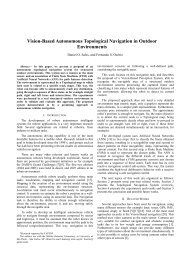
Vision and GPS-based autonomous vehicle navigation using ...

3.2 Template Matching Step
After obtaining the ANN classification, different road templates
are placed over the image in order to identify the road
geometry. One of them identifies a straight road ahead, two
identify soft turns, and two identify hard turns. Each template
is composed of a mask of 1s and 0s, as proposed in
[17]. The value of each mask is multiplied by the correspondent
value into the navigability matrix. The total score for
each template is the sum of products. A good performance
was obtained in the navigation defined by the urban path
avoiding obstacles using the best template [16].
In this step, templates are selected for use in the next step
of the system. The template that obtains the higher score
is selected as the best match to the road geometry.
3.3 Occupation Percentage
In this step, the templates of the previous step are used to
calculate the occupation percentage of the road regions (navigable
and non-navigable). This calculation is performed by
dividing the template score by its maximum value. This is
carried out for each template, so several values normalized
between [0, 1] are obtained.
After obtaining these values based on the occupation areas
resulting from the classified images (navigable and nonnavigable
- image processing step), we verify if the occupation
percentage obtained is lower than a threshold level. It
is then assigned as either obstructed (value 0) or free (value
1) for the occupation areas, which are part of the system
input for the next step.
3.4 Learning Based Navigation
We have already developed works analyzing different levels
of memory of the templates based on examples obtained
from human drivers using neural networks [15]. The results
of these neural networks have also been compared with
different supervised learning techniques for the same purpose
[14]. This work is based in the integration of GPS
and compass, furthermore the occupation percentage on the
autonomous navigation system.
In this step, the basic network structure used is a feedforward
MLP. The activation functions of the hidden neurons
are logistic sigmoid and hyperbolic tangent, and the ANN
learning method is the resilient backpropagation (RPROP).
The inputs are represented by azimuth (difference between
the current and target positions of the vehicle) and the
five values obtained by the occupation percentage step (obstructed
or free occupation areas). The outputs of the proposed
method are the steer angle and speed (Figure 4).
Figure 4: Structure of the second ANN used to generate
steering and acceleration commands.
283
4. EXPERIMENTAL RESULTS
The experiments were performed using CaRINA (Figure
1), an electric vehicle capable of autonomous navigation in
an urban road, equipped with a VIDERE DSG camera, a
ROBOTEQ AX2580 motor controller for steering control, a
TNT Revolution GS Compass (orientation) and a GARMIN
18X-5Hz GPS (localization). The image acquisition resolution
was set to (320 x 240) pixels. Figure 5 shows the vehicle
trajectory obtained by GPS coordinates.
Figure 5: GPS coordinates performed by CaRINA.
Seven GPS waypoints (desired trajectory) were defined.
In order to navigate, the vehicle used a monocular camera to
avoid obstacles. The experiment was successfully performed
as it followed the GPS points and avoided obstacles. In some
of the straight paths, the vehicle had to avoid curbs at the
same time it was attracted by the GPS goal points, resulting
in some oscillation in the final trajectory.
Table 2 shows the values of the path performed by Ca-
RINA. Five different ANNs topologies were analyzed using
two learning functions (logistic sigmoid and hyperbolic tangent).
These topologies represent the architecture of the
second ANN used in our proposed system. Several topologies
of ANNs were tested to obtain the minimum training
error and a near optimal neural architecture.
The ANN architecture was selected considering the number
of neurons in the hidden layer using the RPROP supervised
learning algorithm in MLP networks and considering
the values of MSE (Mean squared error) and the best epoch
(Optimal point of generalization [OPG], i.e., minimum training
error and maximum capacity of generalization).
We also evaluated the ANNs modifying the learning functions.
The main difference between these functions is that
logistic sigmoid produces positive numbers between 0 and 1,
and the hyperbolic tangent (HT), numbers between -1 and
1. Furthermore the HT is the activation function most commonly
used in neural networks. After the analysis of Table
2, the 6x15x2 architecture using the hyperbolic activation
function showed the lowest MSE for the 10600 epoch. Five
different runs were executed changing the random seed used
in the neural networks (Tests 1 to 5).
Figure 6 shows the histograms of the errors based on the
best ANN topology obtained in Table 2. Topologies 4 and
5 were accepted based on the results. Figure 6(b) presents
the error concentrated on zero and with a lower dispersion
than the one in Figure 6(a). The same is true for Figure
6(d), which shows a lower dispersion compared to Figure
6(c), therefore encouraging the use of topology 5.