6. Order Statistics

Order Statistics
http://www.math.uah.edu/stat/sample/OrderStatistics.xhtml
1 of 7 7/16/2009 6:06 AM
Virtual Laboratories > 6. Random Samples > 1 2 3 4 5 6 7
6. Order Statistics
Definitions
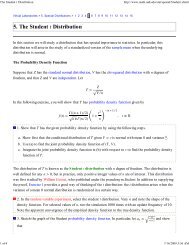
Suppose again that we have a basic random experiment, and that X is a real-valued random variable for the
experiment with distribution function F and probability density function f .
We perform n independent replications of the basic experiment to generate a random sample
X = (X 1 , X 2 , ..., X n ) of size n from the distribution of X. Recall that this is a sequence of independent
random variables, each with the distribution of X.
Let X n, k( X) denote the k th smallest of element of the sample X. This statistics is called the order statistic of
order k. Often the first step in a statistical study is to order the data; thus order statistics occur naturally. Our
goal in this section is to study the distribution of the order statistics in terms of the sampling distribution.
Note in particular that the extreme order statistics are the minimum and maximum values:
X n, 1 = min {X 1 , X 2 , ..., X n }, X n, n = max {X 1 , X 2 , ..., X n }
1. In the order statistic experiment, use the default settings and run the experiment a few times. Note the
following:
a. The table on the left shows the values of the order statistics.
b. The graph on the left shows the density function of the sampling distribution in blue and the sample
values in red.
c. The graph on the right shows the density function of the selected order statistic in blue and the
empirical density function in red. The mean/standard deviation bar of the distribution is shown in blue
while the empirical mean/standard deviation bar is shown in red.
d. The table on the right gives numerical values of the density function and moments and the empirical
density function and moments.
Distributions
The Distribution of the k th Order Statistic
Let G n, k denote the distribution function of X n, k . Define
N n, y = #({i ∈ {1, 2, ..., n} : X i ≤ y}),
y ∈ R
2. Show that N n, y has the binomial distribution with parameters n and F(y) for each y ∈ R.

Order Statistics
http://www.math.uah.edu/stat/sample/OrderStatistics.xhtml
2 of 7 7/16/2009 6:06 AM
3. Show that X n, k ≤ y if and only if N n, y ≥ k for y ∈ R and k ∈ {1, 2, ..., n}.
4. Use the results of Exercises 2 and 3 to show that
n
n
G n, k( y) = ∑ j =k ( j) F(y) j (1 − F(y)) n − j , y ∈ R
5. In particular, show that G n, 1( y) = 1 − (1 − F(y)) n , y ∈ R.
6. In particular, show that G n, n( y) = F(y) n , y ∈ R.
7. Suppose now that X has a continuous distribution. Show that X n, k has a continuous distribution with
probability density function
n
g n, k(y) = ( k − 1, 1, n − k) F(y)k−1 (1 − F(y)) n −k f (y),
Hint: Differentiate the expression in Exercise 4 with respect to y.
y ∈ R
8. In the order statistic experiment, select the uniform distribution on [ 0, 1]
and n = 5. Vary k from 1 to 5
and note the shape of the density function of X n, k . For each value of k, run the simulation 1000 times with
and update frequency of 10. Note the apparent convergence of the empirical density function to the true
density function.
There is a simple heuristic argument for the result in Exercise 7. First, g n, k(y) dy is the probability that X n, k
is in an infinitesimal interval of size dy about y. On the other hand, this event means that one of sample
variables is in the infinitesimal interval, k − 1 sample variables are less than y, and n − k sample variables are
greater than y. The number of ways of choosing these variables is the multinomial coefficient
n
( k − 1, 1, n − k) = n!
(k − 1)! 1! (n − k)!
By independence, the probability that the chosen variables are in the specified intervals is
F(y) k−1 (1 − F(y)) n −k f (y) dy
9. Consider a random sample of size n from the exponential distribution with rate parameter r. Compute
the probability density function of the k th order statistic X n, k . In particular, note that the minimum of the
variables X n, 1 has the exponential distribution with rate parameter n r.
10. In the order statistic experiment, select the exponential (1) distribution and n = 5. Vary k from 1 to 5
and note the shape of the probability density function of X n, k . For each value of k, run the simulation 1000
times with and update frequency of 10. Note the apparent convergence of the empirical density function to
the true density function.

Order Statistics
http://www.math.uah.edu/stat/sample/OrderStatistics.xhtml
3 of 7 7/16/2009 6:06 AM
11. Consider a random sample of size n from the uniform distribution on the interval [ 0, 1]
.
a.
b.
Show that X n, k has beta distribution with parameters k and n − k + 1.
Given the mean and variance of X n, k .
12. In the order statistic experiment, select the uniform distribution on [ 0, 1]
and n = 6. Vary k from 1 to 6
and note the size and location of the mean/standard deviation bar. For each value of k, run the simulation
1000 times with and update frequency of 10. Note the apparent convergence of the empirical moments to
the distribution moments.
13. Four fair dice are rolled. Find the probability density function of each of the order statistics.
14. In the dice experiment, select the following order statistic and die distribution. Increase the number of
dice from 1 to 20, noting the shape of the probability density function at each stage. Now with n = 4, run
the simulation 1000 times, updating every 10 runs. Note the apparent convergence of the relative
frequency function to the density function.
a.
b.
c.
d.
Maximum score with fair dice.
Minimum score with fair dice.
Maximum score with ace-six flat dice.
Minimum score with ace-six flat dice.
Joint Distributions
Suppose again that X has a continuous distribution.
15. Suppose that j < k. Use an heuristic argument to show that the joint density of (X n, j , X n, k) is
n
g n, j, k(y, z) = ( j − 1, 1, k − j − 1, 1, n − k) F(y) j −1 f (y) (F(z) − F(y)) k− j −1 f (z) (1 − F(z)) n −k ,
y < z
Similar arguments can be used to obtain the joint probability density function of any number of the order
statistics. Of course, we are particularly interested in the joint probability density function of all of the order
statistics; the following exercise gives this joint probability density function, which has a remarkably simple
form.
16. Show that (X n, 1 , X n, 2 , ..., X n, n) has joint probability density function given by
g n (y 1 , y 2 , ..., y n ) = n! f (y 1 ) f (y 2 ) ··· f (y n ),
y 1 < y 2 < ··· < y n
a.
b.
For each permutation i = (i 1 , i 2 , ..., i n ) of (1, 2, ..., n), let S i = {x ∈ R n : x i1 < x i2 < ··· < x in }.
On S i , the mapping (x 1 , x 2 , ..., x n ) ↦ (x i1 , x i2 , ..., x in ) is one-to-one, has continuous first partial
derivatives, and has Jacobian 1.

Order Statistics
http://www.math.uah.edu/stat/sample/OrderStatistics.xhtml
4 of 7 7/16/2009 6:06 AM
c.
d.
e.
The sets S i where i ranges over the n! permutations of (1, 2, ..., n) are disjoint.
The probability that (X 1 , X 2 , ..., X n ) is not in one of these sets is 0.
Now use the multivariate change of variables formula.
Again, there is a simple heuristic argument for the formula in Exercise 16. For each y ∈ R n with
y 1 < y 1 < ··· < y n , there are n! permutations of the coordinates of y. The probability density of
(X 1 , X 2 , ..., X n ) at each of the this points is f (y 1 ) f (y 2 ) ··· f (y n ). Hence the probability density of
(X n, 1 , X n, 2 , ..., X n, n) at y is n! times this product.
17. Consider a random sample of size n from the exponential distribution with rate parameter r. Compute
the joint probability density function of the order statistics (X n, 1 , X n, 2 , ..., X n, n) .
18. Suppose that (X 1 , X 2 , ..., X n ) is a random sample of size n from the uniform distribution on the
interval [ a, b]
, where a < b. Show that
a.
b.
(X 1 , X 2 , ..., X n ) is uniformly distributed on [ a,
b]
(X n, 1 , X n, 2 , ..., X n, n) is uniformly distributed on {x ∈ [ a,
b]
n : a < x 1 < x 2 < ··· < x n < b}.
n .
19. Four fair dice are rolled. Find the joint probability density function of the order statistics.
Derived Statistics
We will study several important statistics that are based on order statistics.
Sample Range
The sample range is the random variable
R = X n, n − X n, 1
This statistic gives a simple measure of the dispersion of the sample. Note the distribution of the sample
range can be obtained from the joint distribution of (X n, 1 , X n, n) given earlier.
20. Consider a random sample of size n from the exponential distribution with rate parameter r. Show that
the sample range R has the same distribution as the maximum of a random sample of size n − 1 from this
exponential distribution.
21. Consider a random sample of size n from the uniform distribution on [ 0, 1]
.
a.
Show that R has the beta distribution with left parameter n − 1 and right parameter 2.

Order Statistics
http://www.math.uah.edu/stat/sample/OrderStatistics.xhtml
5 of 7 7/16/2009 6:06 AM
b.
c.
Give the mean and variance of R.
What happens as n → ∞?
22. Four fair dice are rolled. Find the probability density function of the sample range.
The Sample Median
If n is odd, the sample median is the middle of the ordered observations, namely
X n, k where k = n + 1
2
If n is even, there is not a single middle observation, but rather two middle observations. Thus, the median
interval is
[ X n, k , X n, k+1]
where k = n 2
In this case, the sample median is defined to be the midpoint of the median interval
1
2 ( X n, k + X n, k+1) where k = n 2
In a sense, this definition is a bit arbitrary because there is no compelling reason to prefer one point in the
median interval over another. For more on this issue, see the discussion of error functions in the section on
Variance. In any event, sample median is a natural statistic that is analogous to the median of the distribution.
Moreover, the distribution of the sample median can be obtained from our results on order statistics.
Sample Quantiles
We can generalize the sample median discussed above to other sample quantiles. Suppose that p ∈ ( 0, 1)
. Let
k = ⌊(n + 1) p⌋, the integer part of (n + 1) p, and let q = (n + 1) p − k, the fractional part of (n + 1) p. Using
linear interpolation, we define the sample quantile of order p to be
X n, k + q (X n, k+1 − X n, k) = (1 − q) X n, k + q X n, k+1
Once again, the sample quantile of order p is a natural statistic that is analogous to the distribution quantile of
order p. Moreover, the distribution of a sample quantile can be obtained from our results on order statistics.
The sample quantile of order 1 4 is known as the first sample quartile and is frequently denoted Q 1. The the
sample quantile of order 3 4 is known as the third sample quartile and is frequently denoted Q 3. Note that

Order Statistics
http://www.math.uah.edu/stat/sample/OrderStatistics.xhtml
6 of 7 7/16/2009 6:06 AM
the sample median is the quartile of order 1 2 and is sometimes denoted Q 2. The interquartile range is
defined to be
IQR = Q 3 − Q 1
The IQR is a statistic that measures the spread of the distribution about the median, but of course this
number gives less information than the interval [ Q 1 , Q 3 ].
Exploratory Data Analysis
The five statistics (X n, 1 , Q 1 , Q 2 , Q 3 , X n, n) are often referred to as the five-number summary. Together,
these statistics give a great deal of information about the distribution in terms of the center, spread, and
skewness. Graphically, the five numbers are often displayed as a boxplot, which consists of a line extending
from the minimum X n, 1 to the maximum X n, n , with a rectangular box from the first quartile Q 1 to the third
quartile Q 3 and tick marks at the minimum, the median Q 2 , and the maximum.
23. In the interactive histogram, select boxplot. Construct a frequency distribution with at least 6 classes
and at least 10 values. Compute the statistics in the five-number summary by hand and verify that you get
the same results as the applet.
24. In the interactive histogram, select boxplot. Set the class width to 0.1 and construct a distribution with
at least 30 values of each of the types indicated below. Then increase the class width to each of the other
four values. As you perform these operations, note the shape of the boxplot and the relative positions of
the statistics in the five-number summary:
a.
b.
c.
d.
e.
f.
A uniform distribution.
A symmetric, unimodal distribution.
A unimodal distribution that is skewed right.
A unimodal distribution that is skewed left.
A symmetric bimodal distribution.
A u-shaped distribution.
25. In the interactive histogram, select boxplot. Start with a distribution and add additional points as
follows. Note the effect on the boxplot:
a.
b.
c.
d.
e.
f.
Add a point below X n, 1 .
Add a point between X n, 1 and Q 1 .
Add a point between Q 1 and Q 2 .
Add a point between Q 2 and Q 3 .
Add a point between Q 3 and X n, n .
Add a point above X n, n .

Order Statistics
http://www.math.uah.edu/stat/sample/OrderStatistics.xhtml
7 of 7 7/16/2009 6:06 AM
In the last problem, you may have noticed that when you add an additional point to the distribution, one or
more of the five statistics does not change. In general, quantiles can be relatively insensitive to changes in the
data.
26. Compute the five number summary and sketch the boxplot for the velocity of light variable in
Michelson's data. Compare the median with the “true value” of the velocity of light.
27. Compute the five number summary and sketch the boxplot for the density of the earth variable in
Cavendish's data. Compare the median with the “true value” of the density of the earth.
28. Compute the five number summary and sketch the boxplot for the net weight variable in the M&M
data.
29. Compute the five number summary for the sepal length variable in Fisher's iris data, using the cases
indicated below. Plot the boxplots on parallel axes, so you can compare.
a.
b.
c.
d.
All cases
Type Setosa only
Type Verginica only
Type Versicolor only
Virtual Laboratories > 6. Random Samples > 1 2 3 4 5 6 7
Contents | Applets | Data Sets | Biographies | External Resources | Key words | Feedback | ©