7. The Multivariate Normal Distribution

The Multivariate Normal Distributionhttp://www.math.uah.edu/stat/special/MultiNormal.xhtml2 of 5 7/16/2009 5:56 AM6. Show that inverse transformation is given byu = x − μ 1σ 1, v =x − μ 1σ 1 1 − ρ 2√− ρy − μ 2σ 2 1 − ρ 2√7. Show that the Jacobian of the transformation in the previous exercise is∂(u, v)∂(x, y) = 1σ 1 σ 2 1 − ρ 2√Note that the Jacobian is a constant; this is because the transformation is linear.8. Use the previous exercises, the independence of U and V, and the change of variables formula to showthat the joint probability density function of (X, Y) isf (x, y) =12 π σ 1 σ 2 1 − ρ 2√1 (x − μ 1 ) 2exp − ( 2 (1 − ρ 2 ) ( σ2 1(x, y) ∈ R 2− 2 ρ (x − μ 1) (y − μ 2 )σ 1 σ 2+ (y − μ 2) 2σ 22)) ,If c is a constant, the set of points {(x, y) ∈ R 2 : f (x, y) = c} is called a level curve of f (these are curves ofconstant probability density).9. Show thata.b.The level curves of f are ellipses centered at (μ 1 , μ 2 ).The axes of these ellipses are parallel to the coordinate axes if and only if ρ = 010. In the bivariate normal experiment, run the experiment 2000 times with an update frequency of 10 forselected values of the parameters. Observe the cloud of points in the scatterplot and note the apparentconvergence of the empirical density function to the probability density function.TransformationsThe following exercise shows that the bivariate normal distribution is preserved under affine transformations.11. Define W = a 1 X + b 1 Y + c 1 and Z = a 2 X + b 2 Y + c 2 . Use the change of variables formula to showthat (W, Z) has a bivariate normal distribution. Identify the means, variances, and correlation.12. Show that the conditional distribution of Y given X = x is normal with mean and variance given bya.b.(Y|X = x) = μ 2 + ρ σ 2 x−μ 1σ 1var(Y|X = x) = σ 22( 1 − ρ 2 )13. Use the definition of X and Y in terms of the independent standard normal variables U and V to show

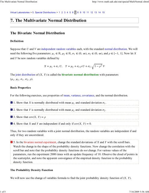
The Multivariate Normal Distributionhttp://www.math.uah.edu/stat/special/MultiNormal.xhtml3 of 5 7/16/2009 5:56 AMthatY = μ 2 + ρ σ X − μ 12 + σ 2σ √1 − ρ 2 V1Now give another proof of the result in Exercise 12 (note that X and V are independent).14. In the bivariate normal experiment, set the standard deviation of X to 1.5, the standard deviation of Yto 0.5, and the correlation to 0.7.a.b.c.Run the experiment 100 times, updating after each run.For each run, compute (Y|X = x) the predicted value of Y for the given the value of X.Over all 100 runs, compute the square root of the average of the squared errors between the predictedvalue of Y and the true value of Y.The following problem is a good exercise in using the change of variables formula and will be useful when wediscuss the simulation of normal variables.15. Recall that U and V are independent random variables each with the standard normal distribution.Define the polar coordinates (R, Θ) of (U, V) by the equations U = R cos(Θ), V = R sin(Θ) where R ≥ 0and 0 ≤ Θ < 2 π. Show thata.b.c.R has probability density function g(r) = r e − 1 2 r 2 , r ≥ 0.Θ is uniformly distributed on [ 0, 2 π).R and Θ are independent.The distribution of R is known as the Rayleigh distribution, named for William Strutt, Lord Rayleigh. Itis a member of the family of Weibull distributions, named in turn for Wallodi Weibull.The General Multivariate Normal DistributionThe general multivariate normal distribution is a natural generalization of the bivariate normal distributionstudied above. The exposition is very compact and elegant using expected value and covariance matrices, andwould be horribly complex without these tools. Thus, this section requires some prerequisite knowledge oflinear algebra. In particular, recall that A T denotes the transpose of a matrix A.The Standard Normal DistributionSuppose that Z = (Z 1 , Z 2 , ..., Z n ) is a vector of independent random variables, each with the standard normaldistribution. Then Z is said to have the n-dimensional standard normal distribution.16. Show that (Z) = 0 (the zero vector in R n ).

The Multivariate Normal Distributionhttp://www.math.uah.edu/stat/special/MultiNormal.xhtml4 of 5 7/16/2009 5:56 AM17. Show that VC(Z) = I (the n×n identity matrix).18. Show that Z has probability density function1g(z) =(2 π) n / 2 exp ( −1 2 z · z ) , z ∈ Rn19. Show that Z has moment generating function given by1(exp(t · Z)) = exp ( 2 t · t ) , t ∈ RnThe General Normal DistributionNow suppose that Z has the n-dimensional standard normal distribution. Suppose that μ ∈ R n and thatA ∈ R n×n is invertible. The random vector X = μ + A Z is said to have an n-dimensional normaldistribution.20. Show that (X) = μ.21. Show that VC(X) = A A T , and that this matrix is invertible and positive definite.22. Let V = VC(X) = A A T . Use the multivariate change of variables theorem to show that X hasprobability density functionf (x) =1(2 π) n / 2 det(V) √23. Show that X has moment generating function given byexp (− 1 2 (x − μ) · V −1 (x − μ) ),x ∈ R n(exp(t · X)) = exp (μ · t + 1 2 t · V t ) ,t ∈ RnNote that the matrix A that occurs in the transformation is not unique, but of course the variance-covariancematrix V is unique. In general, for a given positive definite matrix V, there are many invertible matrices A suchthat A A T = V. A theorem in matrix theory states that there is a unique lower triangular matrix L with thisproperty.24. Identify the lower triangular matrix L for the bivariate normal distribution.TransformationsThe multivariate normal distribution is invariant under two basic types of transformations: affinetransformation with an invertible matrix, and the formation of subsequences.25. Suppose that X has an n-dimensional normal distribution. Suppose also that a ∈ R n and thatB ∈ R n×n is invertible. Show that Y = a + B X has a multivariate normal distribution. Identify the mean

The Multivariate Normal Distributionhttp://www.math.uah.edu/stat/special/MultiNormal.xhtml5 of 5 7/16/2009 5:56 AMvector and the variance-covariance matrix of Y.26. Suppose that X has an n-dimensional normal distribution. Show that any permutation of thecoordinates of X also has an n-dimensional normal distribution. Identify the mean vector and the variancecovariancematrix. Hint: Permuting the coordinates of X corresponds to multiplication of X by apermutation matrix--a matrix of 0's and 1's in which each row and column has a single 1.27. Suppose that X = (X 1 , X 2 , ..., X n ) has an n-dimensional normal distribution. Show that if k < n,W = (X 1 , X 2 , ..., X k ) has a k-dimensional normal distribution. Identify the mean vector and the variancecovariancematrix.28. Use the results of Exercise 26 and Exercise 27 to show that if X = (X 1 , X 2 , ..., X n ) has an n-dimensional normal distribution and if (i 1 , i 2 , ..., i k ) is a sequence of distinct indices, thenW = (X i1 , X i2 , ..., X ik ) has a k-dimensional normal distribution.29. Suppose that X has an n-dimensional normal distribution, a ∈ R m , and that B ∈ R m×n has linearlyindependent rows (thus, m ≤ n). Show that Y = a + B X has an m-dimensional normal distribution. Hint:There exists an invertible n×n matrix C for which the first m rows are the rows of B. Now use Exercise 25and Exercise 27.Note that the results in Exercises 25, 26, 27, and 28 are special cases of the result in Exercise 29.30. Suppose that X has an n-dimensional normal distribution, Y has an m-dimensional normal distribution,and that X and Y are independent. Show that (X, Y) has an m + n dimensional normal distribution. Identifythe mean vector and the variance-covariance matrix.31. Suppose that X is a random vector in R m , Y is a random vector in R n , and that (X, Y) has an m + n-dimensional normal distribution. Show that X and Y are independent if and only if cov(X, Y) = 0 (them×n zero matrix).Virtual Laboratories > 5. Special Distributions > 1 2 3 4 5 6 7 8 9 10 11 12 13 14 15Contents | Applets | Data Sets | Biographies | External Resources | Key words | Feedback | ©