High-Dynamic-Range Laser Amplitude and Phase Noise - Next ...

More documents

Recommendations

Info

648 IEEE JOURNAL ON SELECTED TOPICS IN QUANTUM ELECTRONICS, VOL. 7, NO. 4, JULY/AUGUST 2001 Noise voltage (nV/√Hz) Fig. 6. Measured and calculated electronic noise at the output of the photoreceiver used for amplitude noise measurements. 1 Measured amplitude noise of photoreceiver. Calculated noise at output of photoreceiver based 2 on manufacturer’s data ( ). 3 Measurement system noise floor. Noise Voltage (dBV/√Hz) 1000 100 10 1 0.1 1 10 100 1k 10k 100k 1M 10M Frequency (Hz) -130 -135 -140 -145 -150 -155 -160 -165 -170 -175 -180 0.1 1 10 100 1k 10k 100k 1M 10M 100M Fig. 7. Photoreceiver gain and noise. 1 Relative gain in dB with respect to a 2 nominal gain of 330 V/A. Frequency (Hz) Noise voltage at photoreceiver output. 5 dB. The 120-MHz filter is necessary to reduce the second and higher order harmonics from the photoreceiver since the amplifier cannot tolerate the high peak voltages of the pulses. 1 2 5 0 -5 -10 -15 -20 -25 -30 -35 -40 -45 1 2 3 Relative Gain (dB) VI. THE COMPLETE SYSTEM The essential components for making amplitude and phasenoise measurements are shown in Fig. 1. With the exception of the photoreceiver, these are the same components required to make amplitude and phase-noise measurements of RF and microwave sources. Many years of research and development have gone into optimizing these components and creating integrated measurement systems, including software control. We take advantage of this by using one of the first complete systems developed for phase-noise measurement; the HP 3047A. (These systems are not the same as the “phase-noise measurement utility” available on some spectrum analyzers.) However, it is not necessary to have a commercial system in order to make reliable, high-dynamic-range noise measurements. One can assemble the essential components and, using modern software tools, create an equivalent system. The commercial systems eliminate the arduous tasks associated with measurement calibration, normalization, data acquisition and display, instrument control, and stitching together data from the various frequency bands. The reader is cautioned, however, to realize that replicating and verifying a reliable AM/PM noise measurement system is a formidable project. The software that controls the HP 3047A has in excess of 10 000 lines of BASIC code. The HP 3047A consists of two spectrum analyzers: a spectrum analyzer interface and a computer running the measurement software. The low-frequency FFT analyzer, an HP 3582A, has a frequency range from 0.01 Hz to 25 kHz and a noise floor of 140 dBm/Hz ( 1 kHz). The RF spectrum analyzer, an HP 3585A, covers the range from 20 Hz to 40 MHz and has a noise floor of 147 dBm/Hz ( 20 kHz). Together, these spectrum analyzers allow us to make noise measurements at offset frequencies from 0.02 Hz to 40 MHz. In this range, we readily observe noise with mechanical origins such as optical mount and electrical cable vibrations, instrument fan vibrations, general laboratory acoustical noise coupled into the laser signal, and low-frequency electrical interference such as power line or switching supply spurs (1 Hz–500 kHz). We can also see higher frequency electrical interference, thermal noise, laser relaxation oscillations, shot noise, and more. Since the spectrum analyzers have noise floors approximately 30 dB above thermal noise ( dBm/Hz), a low-noise amplifier is included in the spectrum analyzer interface box (HP 35601A). With 40 dB of gain and a noise figure (NF) of 5 dB ( kHz), the absolute system noise floor is reduced to 169 dBm/Hz and all measured noise, e.g., laser shot noise, must be greater than this value. The interface box also includes a 5 MHz–1.6 GHz mixer used as a phase detector. A 60-MHz LPF is used to remove the second- and higher order harmonics that are present at the output of the phase detector. It is important to use a multipole, constant-impedance LPF so that the large second harmonic signal is not reflected back into the mixer, degrading detector performance, or passed through to the LNA. In addition, there is a remotely programmable phase-locked loop (PLL) for frequency control of voltage-controlled oscillators (VCOs). This allows the system to keep two sources (e.g., mode-locked laser and reference oscillator) in quadrature during a measurement. All of the components of the measurement system must be connected with high-quality cables and connectors. Doubleshielded or semi-rigid coax should be used whenever possible. The instruments and cabling should be securely mounted to minimize microphonic effects, and every effort should be made to minimize ground loops [38].
SCOTT et al.: HIGH-DYNAMIC-RANGE LASER AMPLITUDE AND PHASE NOISE MEASUREMENT TECHNIQUES 649 VII. SYSTEM CALIBRATION One of the most important, and frequently overlooked, elements in making reliable noise measurements is system calibration. It is one of the most difficult and time-consuming aspects of the measurement process. At a minimum, the following must be characterized over the entire frequency range of interest (dc-40 MHz for AM noise and 40–120 MHz for PM noise), photoreceiver and amplifier gain and noise, filter bandwidths, and spectrum analyzer response (noise floor). In addition, for phasenoise measurements, we need to know the phase detector constant, PLL response when using a VCO, absolute phase noise of any reference oscillators, and residual phase noise of all amplifiers used. A. System Amplitude Noise Floor Once a noise measurement system has been assembled, the noise floor must be continually verified. In our experience, when the setup location or environmental conditions change, a noise floor may no longer be valid. Since we are looking at such small signal levels ( 1nV/ Hz), even cable placement can make a 20-dB difference in a spur level. Ground loops are especially troublesome. Good electrical engineering practices must be used [38] during the design and construction of the system. All components and their power supplies must be considered. For amplitude noise measurements, the absolute voltages measured by the spectrum analyzers are compared with the dc voltage at the photoreceiver output, which is proportional to the average photocurrent. The ratio then establishes the relative intensity noise (RIN) as a spectral density (dB/Hz). To observe the full dynamic range available, it is essential that the system noise floor be below that of the photoreceiver, which in turn must be below the shot noise. System noise floor verification is accomplished by terminating the input of the LNA in its characteristic impedance (50 ) and making a full measurement. System and environmental noise sources can then be recognized and minimized. 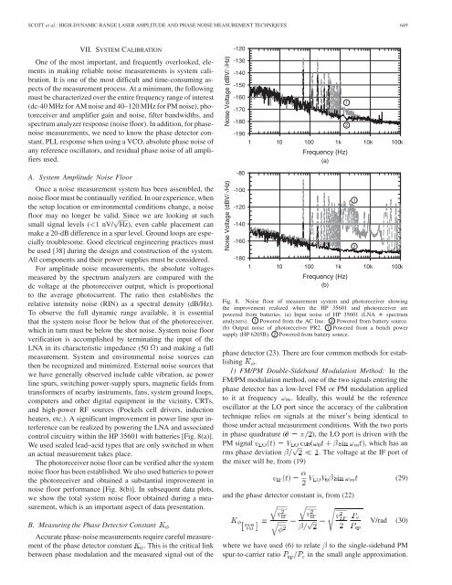External noise sources that we have generally observed include cable vibration, ac power line spurs, switching power-supply spurs, magnetic fields from transformers of nearby instruments, fans, system ground loops, computers and other digital equipment in the vicinity, CRTs, and high-power RF sources (Pockels cell drivers, induction heaters, etc.). A significant improvement in power line spur interference can be realized by powering the LNA and associated control circuitry within the HP 35601 with batteries [Fig. 8(a)]. We used sealed lead–acid types that are only switched in when an actual measurement takes place. The photoreceiver noise floor can be verified after the system noise floor has been established. We also used batteries to power the photoreceiver and obtained a substantial improvement in noise floor performance [Fig. 8(b)]. In subsequent data plots, we show the total system noise floor obtained during a measurement, which is an important aspect of data presentation. B. Measuring the Phase Detector Constant Accurate phase-noise measurements require careful measurement of the phase detector constant . This is the critical link between phase modulation and the measured signal out of the Noise Voltage (dBV/ √Hz) Noise Voltage (dBV/ √Hz) -120 -130 -140 -150 -160 -170 -180 -190 1 10 100 1k 10k 100k Frequency (Hz) (a) -80 -100 -120 -140 -160 -180 1 10 100 1k 10k 100k Fig. 8. Noise floor of measurement system and photoreceiver showing the improvement realized when the HP 35601 and photoreceiver are powered from batteries. (a) Input noise of HP 35601 (LNA + spectrum analyzers). 1 Powered from the AC line. 2 Powered from battery source. (b) Output noise of photoreceiver PR2. 1 Powered from a bench power supply (HP 6205B). 2 Powered from battery source. 1 2 Frequency (Hz) (b) phase detector (23). There are four common methods for establishing . 1) FM/PM Double-Sideband Modulation Method: In the FM/PM modulation method, one of the two signals entering the phase detector has a low-level FM or PM modulation applied to it at frequency . Ideally, this would be the reference oscillator at the LO port since the accuracy of the calibration technique relies on signals at the mixer’s being identical to those under actual measurement conditions. With the two ports in phase quadrature ( ), the LO port is driven with the PM signal , which has an rms phase deviation . The voltage at the IF port of the mixer will be, from (19) and the phase detector constant is, from (22) 1 2 (29) V/rad (30) where we have used (6) to relate to the single-sideband PM spur-to-carrier ratio in the small angle approximation.
Page 1 and 2: IEEE JOURNAL ON SELECTED TOPICS IN
Page 3 and 4: SCOTT et al.: HIGH-DYNAMIC-RANGE LA
Page 7: SCOTT et al.: HIGH-DYNAMIC-RANGE LA
Page 15: SCOTT et al.: HIGH-DYNAMIC-RANGE LA

High-Dynamic-Range Laser Amplitude and Phase Noise - Next ...

You also want an ePaper? Increase the reach of your titles

Delete template?

Save as template?