DERIVATIVE-FREE OPTIMIZATION Algorithms, software and ...

DERIVATIVE-FREE OPTIMIZATION 

Algorithms, software and 

applications 

Nick Sahinidis 

National Energy Technology Laboratory 

Department of Chemical Engineering 

Carnegie Mellon University 

sahinidis@cmu.edu 

Acknowledgments: 

Luis Miguel Rios 

NIH and DOE/NETL 

1

DERIVATIVE-FREE 

OPTIMIZATION 

• Optimization of a function for which 

– derivative information is not symbolically available 

– derivative information is not numerically computable 

• Talk outline 

– Motivation 

– Review of algorithms and software 

– Application to protein-ligand binding 

– Two new algorithms 

2

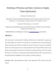
MODEL CALIBRATION 

(Maguthan and Shoemaker, 2005) 

Cl Cl 

Cl C C Cl 

Tetrachloroethene 

H H 

Dechlorination 1 


H Cl 

Cl C C Cl 

Trichloroethene 

Cl C C Cl 

cis-1,2-Dichloroethene 

H H 

C C 

H H 

Ethene 



H 

Cl C C 

H 

H 

Vinyl Chloride 

Parameter estimation problem on top of PDEs 

Each function evaluation takes 2.5 hours 

3

APPLICATIONS 

• Parameter estimation over differential 

equations 

• Optimal control problems 

• Simulation-based optimization 

– Objective computation may involve sampling 

• Automatic calibration of optimization 

algorithms 

• Experimental design/optimization 

4

TIMELINE OF INNOVATION 

5

MOST CITED WORKS 

6


OPTIMIZATION ALGORITHMS 

• LOCAL SEARCH METHODS 

– Direct local search 

» Nelder-Mead simplex 

algorithm 

» Generalized pattern 

search and generating 

search set 

– Based on surrogate 

models 

» Trust-region methods 

» Implicit filtering 

• GLOBAL SEARCH METHODS 

– Deterministic global search 

» Lipschitzian-based partitioning 

» Multilevel coordinate search 

– Stochastic global optimization 

» Hit-and-run 

» Simulated annealing 

» Genetic algorithms 

» Particle swarm 

– Based on surrogate models 

» Response surface methods 

» Surrogate management 

framework 

» Branch-and-fit 

7

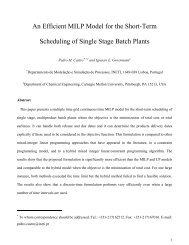
NELDER-MEAD SIMPLEX 

ALGORITHM 

x e 

Expansion 

x r 

x 1 

x co 

Reflection 

x c 

Contraction outside 

x ci 

x 2 

x 3 

Contraction inside 

8

PATTERN SEARCH ALGORITHMS 

9

start 

DIRECT ALGORITHM 

Identify potentially 

optimal 

Evaluate and divide 

Iteration 

1 

BIG partitions and/or LOW function values are preferable 

Iteration 

2 

Iteration 

3 

10

ALGORITHMIC COMPONENTS 

• Random elements 

– Deterministic vs. stochastic 

• Set of points considered in each iteration 

– None; One; Many 

• Partitioning 

– Without: local optimality 

» Torczon (1991) 

– With: global optimality, provided search is “dense” 

11


OPTIMIZATION SOFTWARE 

LOCAL SEARCH 

FMINSEARCH (Nelder-Mead) 

DAKOTA PATTERN (PPS) 

HOPSPACK (PPS) 

SID-PSM (Simplex gradient PPS) 

NOMAD (MADS) 

DFO 

(Trust region, quadratic model) 

IMFIL (Implicit Filtering) 

BOBYQA 


NEWUOA 


GLOBAL SEARCH 

DAKOTA SOLIS-WETS (Direct) 

DAKOTA DIRECT (DIRECT) 

TOMLAB GLBSOLVE (DIRECT) 

TOMLAB GLCSOLVE (DIRECT) 

MCS (Multilevel coordinate search) 

TOMLAB EGO (RSM using Kriging) 

TOMLAB RBF (RSM using RBF) 

SNOBFIT (Branch and Fit) 

TOMLAB LGO (LGO algorithm) 

STOCHASTIC 

ASA (Simulated annealing) 

CMA-ES (Evolutionary algorithm) 

DAKOTA EA (Evolutionary 

algorithm) 

GLOBAL (Clustering - Multistart) 

PSWARM (Particle swarm) 

12

SOLVERS CONSIDERED 

13

SEARCH PROGRESS 

FOR camel6 

14

SEARCH PROGRESS 

FOR camel6—Continued 

15

TEST PROBLEMS 

16

TEST PROBLEM 

CHARACTERISTICS 

Over 500 problems 

17

EXPERIMENTAL SETUP 

• For all solvers 

– Default settings / non-intrusive interface 

– Same bounds; only if required by solver; mostly [-10000, 10000] 

– Same starting points 

– Limit of 2500 iterations and 600 CPU seconds 

• BARON and LINDOGlobal used to find global solutions 

for all problems 

• Absolute Tolerance of 0.01 or Relative Tolerance of 1% 

used for solver comparisons 

• Average-case comparisons based on median objective 

function value of 10 runs from randomly generated 

starting points 

– But DAKOTA/DIRECT, MCS, TOMLAB/CLUSTER 

18

QUESTIONS ADDRESSED 

• What is the quality of solutions obtained by 

current solvers for a given limit on the 

number of allowable function evaluations? 

• Does quality drop significantly as problem 

size increases? 

• Which solver is more likely to obtain global or 

near-global solutions for nonconvex 

problems? 

• Is there a subset of existing solvers that 

would suffice to solve a large fraction of 

problems? 

19

FRACTION OF PROBLEMS SOLVED: 

CONVEX SMOOTH 

20


CONVEX NONSMOOTH 

21


NONCONVEX SMOOTH 

22


NONCONVEX NONSMOOTH 

23

FRACTION OF PROBLEMS 

SOLVER WAS BEST: 

CONVEX SMOOTH 

24




25




26




27


1 TO 2 VARIABLES 

28



29



30



31

STARTING POINT IMPROVEMENT 

• For a given τ between 0 and 1, and a given 

starting point x 0 , a solver improves the 

starting point if 

where f L is the best possible solution for the 

problem 

• Problem considered solved if one or more 

runs satisfied this requirement 

32

FRACTION OF PROBLEMS IMPROVED: 

CONVEX SMOOTH 

33



34



35



36


MULTISTART STRATEGY 

1 to 2 

variables 

3 to 9 

variables 

10 to 30 

variables 

31 to 300 

variables 

37

MINIMUM SET OF SOLVERS 

CONVEX SMOOTH PROBLEMS 

38


CONVEX NONSMOOTH PROBLEMS 

39


NONCONVEX SMOOTH PROBLEMS 

40


NONCONVEX NONSMOOTH PROBLEMS 

41


ALL PROBLEMS 

42

REFINEMENT ABILITY 

• Solvers were started from an starting point 

close to a global minimum of the problem 

• A range of 0.2 for each variable was used 

(unless problem bounds were tighter) 

43

FRACTION OF LOCAL PROBLEMS 

SOLVED: ALL PROBLEMS 

44

MODEL-AND-SEARCH 

LOCAL ALGORITHM 

Π 

x 3 

x 1 

x 5 

r 1 

r 1 

r 2 

r 1 

r 2 

x 2 

r 2 

x 4 

Collect points 

around current 

iterate 

Scale and shift 

origin to current 

iterate 

Add points: n 

linearly 

independent points 

Check for positive 

basis. Add points if 

necessary 

Build and optimize 

interpolating 

model 

Evaluate points in 

specific order 

45

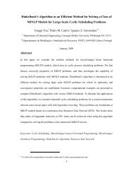
BRANCH-AND-MODEL 

GLOBAL ALGORITHM 

Partition the space 

as a collection H of 

hypercubes 

Reduce H to 

potentially optimal 

set O 

For hypercubes in 

O, FIT models 

Sort O by size of 

hypercubes. 

Evaluate n 2 points 

Sort O by 

predicted optimal 

values. Evaluate n 1 

points 

Optimize models in 

O 

46

PROTEIN-LIGAND DOCKING 

• Identify binding site and pose 

• Conformation must minimize binding free 

energy 

• Docking packages 

– AutoDock, Gold, FlexX … 

– Most rely on genetic and other stochastic search algorithms 

47

BINDING ENERGIES 

B&M outperformed AutoDock in 11 out of 12 cases, 

and found the best solution amongst all solvers for 3 complexes 

48

CONCLUSIONS 

• MCS, LGO, and NEWOA/BOBYQA stand out 

• Stochastic solvers do not perform as well as 

deterministic ones 

– CMA-ES and PSWARM are occasionally competitive 

• Many opportunities 

– New algorithms needed 

– Applications abound 

• Readings 

– Rios and Sahinidis (2010) 

– Conn, Scheinberg and Vicente (2009) 

49

DERIVATIVE-FREE OPTIMIZATION Algorithms, software and ...

Create successful ePaper yourself

Delete template?

Save as template?