Parameter estimation for stochastic equations with ... - samos-matisse

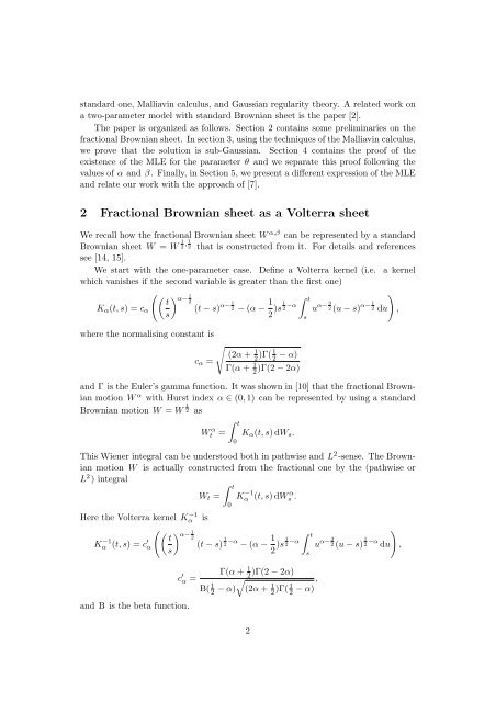
standard one, Malliavin calculus, and Gaussian regularity theory. A related work on
a two-parameter model with standard Brownian sheet is the paper [2].
The paper is organized as follows. Section 2 contains some preliminaries on the
fractional Brownian sheet. In section 3, using the techniques of the Malliavin calculus,
we prove that the solution is sub-Gaussian. Section 4 contains the proof of the
existence of the MLE for the parameter θ and we separate this proof following the
values of α and β . Finally, in Section 5, we present a different expression of the MLE
and relate our work with the approach of [7].
2 Fractional Brownian sheet as a Volterra sheet
We recall how the fractional Brownian sheet W α,β can be represented by a standard
Brownian sheet W = W 1 2 , 1 2 that is constructed from it. For details and references
see [14, 15].
We start with the one-parameter case. Define a Volterra kernel (i.e. a kernel
which vanishes if the second variable is greater than the first one)
( ( ) t α−
1
∫ )
2
K α (t, s) = c α (t − s)
α− 1 1
t
2 − (α −
s
2 )s 1 2 −α u α− 3 2 (u − s)
α− 1 2 du ,
where the normalising constant is
√
(2α + 1 2
c α =
)Γ( 1 2 − α)
Γ(α + 1 2
)Γ(2 − 2α)
and Γ is the Euler’s gamma function. It was shown in [10] that the fractional Brownian
motion W α with Hurst index α ∈ (0, 1) can be represented by using a standard
Brownian motion W = W 1 2 as
W α t =
∫ t
0
K α (t, s) dW s .
This Wiener integral can be understood both in pathwise and L 2 -sense. The Brownian
motion W is actually constructed from the fractional one by the (pathwise or
L 2 ) integral
Here the Volterra kernel K −1
α
Kα
−1 (t, s) = c ′ α
W t =
is
( ( t
s) α−
1
2
(t − s)
1
c ′ α =
and B is the beta function.
∫ t
0
K −1
α (t, s) dW α s .
2 −α − (α − 1 2 )s 1 2 −α ∫ t
Γ(α + 1 2
)Γ(2 − 2α)
√
,
B( 1 2 − α) (2α + 1 2 )Γ( 1 2 − α)
2
s
s
u α− 3 2 (u − s)
1
2 −α du
)
,