Parameter estimation for stochastic equations with ... - samos-matisse
Parameter estimation for stochastic equations with ... - samos-matisse
Parameter estimation for stochastic equations with ... - samos-matisse

Create successful ePaper yourself
Turn your PDF publications into a flip-book with our unique Google optimized e-Paper software.
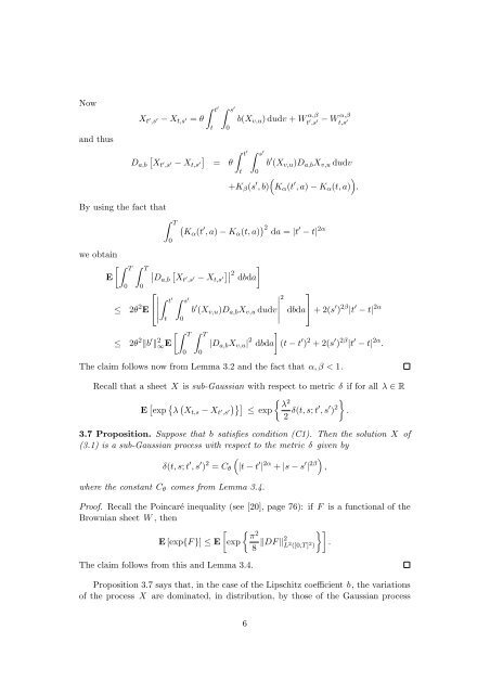
Now<br />
and thus<br />
X t ′ ,s ′ − X t,s ′ = θ ∫ t ′<br />
D a,b<br />
[<br />
Xt ′ ,s ′ − X t,s ′ ]<br />
t<br />
∫ s ′<br />
0<br />
b(X v,u ) dudv + W α,β<br />
t ′ ,s<br />
− W α,β<br />
′ t,s ′<br />
∫ t ′ ∫ s ′<br />
= θ b ′ (X v,u )D a,b X v,u dudv<br />
t 0<br />
(<br />
)<br />
+K β (s ′ , b) K α (t ′ , a) − K α (t, a) .<br />
By using the fact that<br />
∫ T<br />
we obtain<br />
[∫ T<br />
E<br />
≤<br />
≤<br />
0<br />
∫ T<br />
0<br />
⎡<br />
2θ 2 E ⎣<br />
∣<br />
0<br />
(<br />
Kα (t ′ , a) − K α (t, a) ) 2 da = |t ′ − t| 2α<br />
]<br />
∣ [<br />
∣D a,b Xt ′ ,s ′ − X ]∣<br />
t,s ∣<br />
2 ′ dbda<br />
∫ t ′ ∫ s ′<br />
t<br />
0<br />
b ′ (X v,u )D a,b X v,u dudv<br />
∣<br />
2<br />
⎤<br />
dbda⎦ + 2(s ′ ) 2β |t ′ − t| 2α<br />
[∫ T ∫ T<br />
]<br />
2θ 2 ‖b ′ ‖ 2 ∞E |D a,b X v,u | 2 dbda (t − t ′ ) 2 + 2(s ′ ) 2β |t ′ − t| 2α .<br />
0 0<br />
The claim follows now from Lemma 3.2 and the fact that α, β < 1.<br />
Recall that a sheet X is sub-Gaussian <strong>with</strong> respect to metric δ if <strong>for</strong> all λ ∈ R<br />
E [ exp { λ ( { }<br />
)}] λ<br />
2<br />
X t,s − X t ′ ,s ′ ≤ exp<br />
2 δ(t, s; t′ , s ′ ) 2 .<br />
3.7 Proposition. Suppose that b satisfies condition (C1). Then the solution X of<br />
(3.1) is a sub-Gaussian process <strong>with</strong> respect to the metric δ given by<br />
δ(t, s; t ′ , s ′ ) 2 = C θ<br />
(|t − t ′ | 2α + |s − s ′ | 2β) ,<br />
where the constant C θ comes from Lemma 3.4.<br />
Proof. Recall the Poincaré inequality (see [20], page 76): if F is a functional of the<br />
Brownian sheet W , then<br />
[ { }]<br />
π<br />
2<br />
E [exp{F }] ≤ E exp<br />
8 ‖DF ‖2 L 2 ([0,T ] 2 )<br />
.<br />
The claim follows from this and Lemma 3.4.<br />
Proposition 3.7 says that, in the case of the Lipschitz coefficient b, the variations<br />
of the process X are dominated, in distribution, by those of the Gaussian process<br />
6