Parameter estimation for stochastic equations with ... - samos-matisse

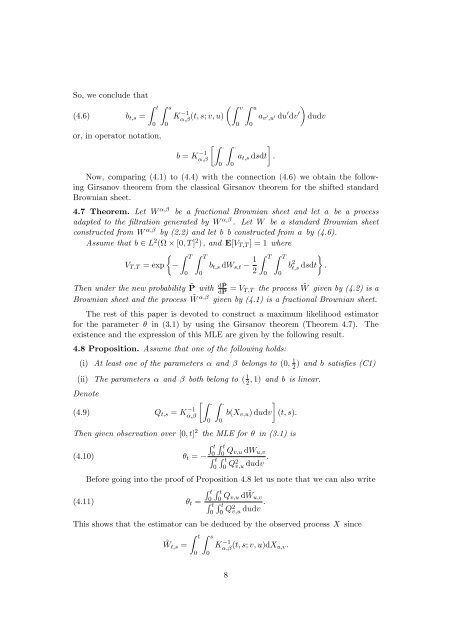
So, we conclude that
(4.6) b t,s =
∫ t ∫ s
or, in operator notation,
0
0
K −1
α,β (t, s; v, u) (∫ v
b = K −1
α,β
[∫ ·
0
∫ ·
0
0
∫ u
0
]
a t,s dsdt .
a v ′ ,u ′ du′ dv ′ )
dudv
Now, comparing (4.1) to (4.4) with the connection (4.6) we obtain the following
Girsanov theorem from the classical Girsanov theorem for the shifted standard
Brownian sheet.
4.7 Theorem. Let W α,β be a fractional Brownian sheet and let a be a process
adapted to the filtration generated by W α,β . Let W be a standard Brownian sheet
constructed from W α,β by (2.2) and let b b constructed from a by (4.6).
Assume that b ∈ L 2 (Ω × [0, T ] 2 ), and E[V T,T ] = 1 where
{ ∫ T ∫ T
V T,T = exp − b t,s dW s,t − 1 ∫ T ∫ T
}
b 2 t,s dsdt .
2
0
0
Then under the new probability ˜P with d ˜P
dP = V T,T the process ˜W given by (4.2) is a
Brownian sheet and the process ˜W α,β given by (4.1) is a fractional Brownian sheet.
The rest of this paper is devoted to construct a maximum likelihood estimator
for the parameter θ in (3.1) by using the Girsanov theorem (Theorem 4.7). The
existence and the expression of this MLE are given by the following result.
4.8 Proposition. Assume that one of the following holds:
(i) At least one of the parameters α and β belongs to (0, 1 2
) and b satisfies (C1)
(ii) The parameters α and β both belong to ( 1 2
, 1) and b is linear.
Denote
(4.9) Q t,s = K −1
α,β
[∫ ·
0
∫ ·
0
]
b(X v,u ) dudv (t, s).
Then given observation over [0, t] 2 the MLE for θ in (3.1) is
(4.10) θ t = −
∫ t ∫ t
0
∫ t
0
0
0 Q v,u dW u,v
∫ t
0 Q2 v,u dudv .
Before going into the proof of Proposition 4.8 let us note that we can also write
(4.11) θ t =
∫ t ∫ t
0
∫ t
0
0 Q v,u d ˜W u,v
∫ t
0 Q2 v,u dudv .
This shows that the estimator can be deduced by the observed process X since
˜W t,s =
∫ t ∫ s
0
0
K −1
α,β (t, s; v, u)dX u,v.
0
8