Table of Contents - California Air Resources Board

Standard Operating Procedure
for
Routine Operation of the
CRPAQS Particle Sizing System
DRAFT
April 18, 2001
Prepared By:
Aerosol Dynamics, Inc.
2329 Fourth St.
Berkeley, CA 94710
Contacts: Susanne Hering, Brent Kirby
(510) 649-9360
1

Table of Contents
1. Scope and Applicability....................................................................... 5
2. Summary of Method........................................................................... 5
2.1. Method Parameters ...................................................................... 5
2.2. System Overview.......................................................................... 5
2.3. The TSI Scanning Mobility Particle Sizer .......................................... 6
2.4. Optical Particle Counters............................................................... 7
2.5. Inlet .......................................................................................... 7
3. Definitions........................................................................................ 8
4. Health and Safety Warnings................................................................. 9
4.1. Laser......................................................................................... 9
4.2. Radioactive Source ....................................................................... 9
5. Cautions .......................................................................................... 9
6. Interferences..................................................................................... 9
7. Personnel Qualifications ...................................................................... 9
8. Apparatus and Materials ..................................................................... 9
9. Site and Equipment Preparation .......................................................... 11
9.1. General Setup ............................................................................ 11
9.2. SMPS Setup Guide ...................................................................... 11
9.2.1. Assembly.............................................................................. 11
9.2.2. Plumbing.............................................................................. 11
9.2.3. Electrical .............................................................................. 11
9.2.4. Power Up ............................................................................. 12
10. Instrument Calibration..................................................................... 12
10.1. Overview ................................................................................. 12
10.2. Particle Sizing Calibration Materials.............................................. 12
10.3. Nebulization System ................................................................... 13
10.4. PSL Calibration Procedure .......................................................... 13
10.4.1. Overview ............................................................................ 13
10.4.2. Preparation of Solutions .......................................................... 13
10.4.3. Instrument Setup ................................................................... 14
10.4.4. Calibration Check Procedure .................................................... 14
10.4.5. Calibration Shutdown Procedure................................................ 15
11. Instrument Operation: Optical Particle Counters ................................... 20
11.1. Daily Checks ............................................................................ 20
11.1.1. Climet SPECTRO .3 .............................................................. 20
11.1.2. PMS LASAIR 1003 ............................................................... 20
3

11.2. Monthly Checks ........................................................................ 21
11.2.1. Flow check .......................................................................... 21
11.2.2. Leak check .......................................................................... 21
11.3. Restart Procedure...................................................................... 22
12. Instrument Operation: Scanning Mobility Particle Sizer .......................... 22
12.1. Daily Checks ............................................................................ 22
12.2. 3-Day Essential Maintenance........................................................ 23
12.2.1. Maintenance Frequency........................................................... 23
12.2.2. Reset TSI Software ................................................................ 23
12.2.3. Rezero ESC Flow Transducers.................................................. 23
12.2.4. Clean Impactor ..................................................................... 24
12.3. Weekly Checks.......................................................................... 24
12.4. Monthly Checks ........................................................................ 25
12.4.1. Flow Check ......................................................................... 25
12.4.2. Leak Check ......................................................................... 26
12.5. Restart Procedure...................................................................... 26
13. Sample Preparation, Handling, and Preservation ................................... 30
14. Preventative Maintenance and Repairs................................................. 30
15. Troubleshooting .............................................................................. 30
15.1. LASAIR Warning Messages......................................................... 30
15.1.1. Power Interruption................................................................. 30
15.1.2. Low Flow ........................................................................... 30
15.1.3. Low Laser Level ................................................................... 30
15.2. OPC Flow Rate Errors ............................................................... 30
15.3. OPC Leak Check Errors ............................................................. 31
15.4. Instrument Manuals................................................................... 31
16. Data Acquisition, Calculations, and Data Reduction ............................... 31
16.1. Raw Data................................................................................. 31
16.2. Reduced Data ........................................................................... 32
16.3. Optical Calibrations ................................................................... 33
17. Computer Hardware and Software...................................................... 35
18. Data Management and Records Management ........................................ 35
19. References ..................................................................................... 35
Appendix A .........................................................................................37
Appendix B..........................................................................................55
Appendix C .........................................................................................69
Appendix D .........................................................................................73
4

1. Scope and Applicability
This applies to the operation of the CRPAQS particle sizing system. This system
measures the ambient particle size distribution, defined as the number concentration of
particles as a function of particle diameter. The system is comprised of the following
instruments:
• Climet Instruments model SPECTRO .3
• Particle Measuring Systems model LASAIR 1003
• TSI Scanning Mobility Particle Sizer model 3936 (SMPS)
These instruments sample from a common inlet system. Together they provide size
distributions from 0.01 to 10 µm particle diameter. This document describes the
common inlet, the individual instruments and their operation, and the calibration
procedures for the combined system.
2. Summary of Method
2.1. Method Parameters
The particle sizing instruments have multiple size bins that span the measured size
range. The number of bins (or channels) and the size range of each are different for the
three sizing instruments. All three instruments output the particle number or number
concentration for each size bin. The parameters for each instrument, as operated for
CRPAQS are listed below.
Measured Parameter: Particle number concentrations units of #/cm 3 per size bin.
Size Bins:
• Climet: 16 channels from 0.3 to 10 µm
• LASAIR: 8 channels from 0.1 to 2 µm
• SMPS: 53 channels from 0.01 to 0.4 µm
Time Resolution: 5 min
Sample flow rates:
• Climet: 1 L/min
• LASAIR: 0.03 L/min
• SMPS: 1 L/min
2.2. System Overview
The particle sizing system is comprised of a common inlet, and three particle sizing
instruments. Each of the three instruments covers a different size range. Particles in the
size range from 0.01 to 0.4 µm are measured by electrical mobility using the TSI
Scanning Mobility Particle Sizer model 3936. For singly charged, spherical particles
the mobility size equals the physical size of the particle. The intermediate size range,
from 0.1 to 2 µm diameter, is measured by the Particle Measuring Systems model
LASAIR 1003. The large particle size range, 0.3 to 10 µm, is measured by the Climet
Instruments model SPECTRO .3. Both the LASAIR and Climet are optical particle
5

counters (OPC’s). Their sizing is based on amount of the light scattered by individual
particles and is dependent on particle refractive index as well as size. All three
instruments sample from downstream of a common PM10 inlet. The inlet, sample lines,
and flow rates were designed to ensure representative sampling by each of the three
instruments for their respective size ranges, as described in Section 2.5. The data must
be combined to yield a complete size distribution.
The selection of the Climet for large particle sizing was based on laboratory evaluation
and comparison of several candidate instruments. Indeed, in the first evaluation none of
the candidate instruments were deemed acceptable (see Appendix A). Two of the
instruments were modified by the manufacturer based on input from Aerosol Dynamics,
and retested. Of these the Climet 0.3 operated at a sample flow of 1 L/min was
considered the most suitable for this study because it did not show false counts at large
particle sizes, and is relatively insensitive to particle refractive index (see Appendix B).
The selection of the SMPS and LASAIR instruments was based on a review of
instrument performance specifications in concert with the expected size distributions
expected for California’s central valley, as described in Appendices C and D,
respectively.
The inlet and the operational principal of each instrument are described in Sections 2.3,
2.4, and 2.5.
2.3. The TSI Scanning Mobility Particle Sizer
The Scanning Mobiltiy Particle Sizer (SMPS) used for CRPAQS is the TSI model
3936. As installed for CRAPQS, it consists of:
• Long Differential Mobility Analyzer model 3081 (LDMA)
• Electrostatic Classifier model 3080 (ESC: DMA control box)
• Condensation Particle Counter model 3010 (CPC)
• Windows 95 computer with TSI SMPS software installed
The SMPS measures the aerosol number size distribution from slightly less than 10 nm
to just under 400 nm particle diameter. One size distribution is reported every five
minutes with resolution of 32 channels per decade of particle diameter.
The SMPS consists of a particle charger/neutralizer, a differential mobility analyzer
(DMA) and a condensation particle counter (CPC) in series. As the sampled aerosol
passes through the radioactive charger (Kr-85) it acquires a known steady-state charge
distribution. Within the DMA the charged aerosol is pulled across a layer of clean air
by an applied electric field while flowing down the length of the annular gap between
two concentric tubes. Particles of different electric mobilities follow different paths and
the DMA selects only that fraction of positively charged particles having electric
mobilities within a narrow window. Most of the selected particles will have one positive
charge with a relatively small fraction having two (or more) positive charges. The CPC
then measures the concentration of the selected aerosol by condensing butanol vapor
onto the particles and growing them to a size large enough to be detected and counted
optically as they pass through a laser beam. Over a period of a few minutes the
selection window of the DMA is scanned from the minimum to the maximum selectable
6

particle size and the CPC count is recorded in tenth of a second increments. Theoretical
relationships are used to convert from scan time to electric mobility to particle
diameter. Knowledge of the charge distribution is used to convert measured
concentrations of charged particles to total concentration at each particle size.
Correction for multiply charged particles is also possible. Within each five-minute
period, two scans are made and summed and the size distribution reported with
resolution of 32 channels per decade of particle diameter.
A dedicated computer running the Windows 95 operating system acts as an
intermediary between the SMPS and the site Data Acquisition System. For details, see
Section 17, Computer Hardware and Software.
2.4. Optical Particle Counters
The particle sizing system has two optical particle counters (OPC’s), the Particle
Measuring Systems model LASAIR 1003 for the intermediate size range, and the
Climet Instruments model SPECTRO .3 for the large particle size range. The OPC’s
report the number of particles counted within fixed size bins. The Climet SPECTRO
covers a size range 0.3-10 µm using 16 channels while the PMS LASAIR covers a size
range of 0.1-2 µm using eight channels. The highest channel records all particles
exceeding the upper limit of the sizing range.
The OPC determines the size of a sampled particle by the quantity of light scattered by
the particle and focused on to a photodetector using a system of mirrors. Since the
amount of light scattered from a particle is a strong function of its size, precise and
repeatable sizing of particles is possible. Particle concentrations are kept low enough
within the measuring volume of the counter to insure only one particle is measured at a
time. The indicated size by an OPC depends on a particle’s refractive index in addition
to its size. An appropriate optical calibration for use in the field is therefore required
for accurate sizing of ambient particles.
2.5. Inlet
The sampling inlet system for the particle sizing instruments is designed to ensure
representative sampling by each instrument. The different particle size ranges measured
by each instrument impose correspondingly different requirements, and these are taken
into account in the design. First, it is necessary that there be no size bias in the size of
particles aspirated into the sampling line over the entire size range from 0.01-10µm.
Second, the flow splits and transport lines to each instrument are designed to minimize
losses for the specific size range covered by that instrument.
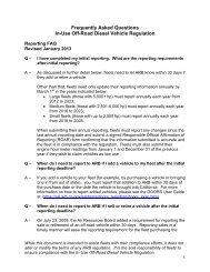
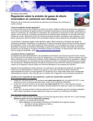
The inlet system for the CRAPQS particle sizing system is shown in Figure 1. Essential
components of the inlet system are:
• PM10 inlet.
• Straight flow path and an isokinetic flow split for the Climet (large particle size
range).
• Transport flow to the LASAIR to minimize gravitational and diffusional losses.
7

• Sufficient flow to the SMPS to minimize diffusional losses.
TSI
SMPS
PARTICLE SIZING INSTRUMENTS
SAMPLING INLET SYSTEM
¼”OD
TSI Flexible,
Conducting
Black Tubing
PMS
LASAIR
ISO-KINETIC
SAMPLING INLET
¼”OD
1¼”OD
½”OD
¼”OD
CLIMET
SPECTRO
Figure 1. Sampling inlet system for particle sizing instruments.
Roof
PM-10 Head
Vent
Valve
Transport
PSL Test
System
Vaccum
The PM10 inlet was needed to provide representative sampling of coarse particles from
the atmosphere, regardless of ambient wind speeds. Without this inlet, the efficiency
with which particles entered the sample line would depend on wind speed, and could
vary with sampling location as well as particle size. The inlet was essential for
comparison of coarse particle size distributions measured on the tower sites to those
measured at ground level. The sample line to the Climet was made to be straight as
possible, with an isokinetic flow split, to ensure representative sampling of the particles
that penetrate the PM10 inlet. Transport flow to the LASAIR counter is supplied by the
SMPS system, thereby minimizing gravitational and diffusional losses to this counter.
3. Definitions
• ADI: Aerosol Dynamics, Inc.
• CPC: Condensation Particle Counter
8

• CRPAQS: California Regional Particulate Air Quality Study
• DMA: Differential Mobility Analyzer
• ESC: Electrostatic Classifier
• LDMA: Long Differential Mobility Analyzer
• OPC: Optical Particle Counter
• PM10 inlet: A standard precut device to select particles of less than 10-µm diameter
• PMS: Particle Measuring Systems
• PSL: Polystyrene Latex
• SMPS: Scanning Mobility Particle Sizer
4. Health and Safety Warnings
4.1. Laser
The LASAIR contains a HeNe laser, and exposure to the direct or scattered laser light
should be avoided.
4.2. Radioactive Source
The TSI SMPS contains a Kr85 radioactive source.
5. Cautions
The pump for the CPC should be exhausted outside, well away from any hydrocarbon
canister samplers.
None.
6. Interferences
7. Personnel Qualifications
The system requires a technically experienced operator who understands the system, its
operation and calibration. This operating procedure assumes the operator can properly
use flow standards and is familiar with computer operations.
Inlet consisting of:
8. Apparatus and Materials
• PM10 inlet
• downtube
• flow splitter, plumbing and electrically conducting flexible tubing
• bypass flow line with rotameter and pump
Climet Spectro 0.3
Particle Measuring Systems LASAIR 1003
TSI SMPS system consisting of:
9

• TSI Scanning Mobility Particle Sizer model 3936 (SMPS)
• Long Differential Mobility Analyzer model 3081 (LDMA)
• Electrostatic Classifier model 3080 (ESC: DMA control box)
• Condensation Particle Counter model 3010 (CPC)
• Windows 95 computer with TSI SMPS software installed
PSL Calibration system consisting of:
• compressed dry air source (such as cylinder of dry air)
• nebulizer setup, with metered dilution and nebulizing air flows
Supplies as listed in Table 1.
Table 1. Field Operations Supply List
1 Initially order 6 Liters HPLC grade butanol
e.g. Fisher HPLC Butanol (cat. # A383-1) Order from Fisher Scientific (1-800-766-7000)
2 Small quantity of spectroscopic grade acetone (for PMS optics cleaning)
e.g. Fisher Optima Acetone (Cat # A929-1) Order from Fisher Scientific (1-800-766-7000)
3 Five latex particle sizes in 15 ml bottles from Interfacial Dynamics
(prices range from $85-135 per):
Dp (µm) Product # Batch # Order 1 of each size from:
0.234 1-200 1063,1 Interfacial Dynamics Corp.
0.576 1-600 684,3 17300 SW Upper Boones Ferry Road,
Suite 120
0.885 1-900 10-200-
Portland, OR 97224
60,1
1.418 1-1400 928,1 Ph: 800-323-4810
4.6 1-4500 736,3 Fax: 503-684-09559
4 5 dozen Devilbiss Micro-Mist Disposable Nebulizers
Product # 4650D-620 Available from many medical supply houses
Mail order: Shield Healthcare (800-675-8840)
5 Dry compressed air cylinder and regulator
Cylinder of dry air (size 1A) for CG-590 regulator. Note -- medical air takes a different
regulator, you don't want this. Order from compressed gas distributor near site
6 Glassware: 10 ml graduated cylinder (2 ea.), 50 ml beakers (5 ea.)
7 Q-tips, Kimwipes, alcohol and distilled water bottles, cleaning detergent
10

9. Site and Equipment Preparation
9.1. General Setup
The site should be prepared with PM10 inlet and sampling system as shown in
Figure 1. The Climet is situated directly underneath the downtube. The LASAIR should
be placed alongside the Climet. These are installed in accordance with their respective
manuals. They each require separate data lines to the data acquisition computer.
Guidance on the setup of the SMPS is given in Section 9.2, with reference to specific
pages in the manual.
9.2. SMPS Setup Guide
9.2.1. Assembly
Assemble the DMA (long tube) including the side support bracket to the ESC (box)
following the instructions on pages 2-9 of the ESC manual. Connect the high voltage
cable (ESC manual pages 2-16). Install the neutralizer (ESC manual pages 2-5, skip
step 3). Install the impactor (ESC manual pages 2-7).
9.2.2. Plumbing
Connect the precut black conductive tubing to the DMA, ESC and CPC following the
schematic (Figure 3-2) on pages 3-6 of the SMPS manual. Note that the filter in front
of the CPC need not be installed for normal use as the connecting valve is normally
closed.
The vacuum pump (small diaphragm) should be located near the SMPS (not outside) as
routine procedures require short-term shut down and it is not very noisy. Connect the
vacuum hose provided (thick-wall Tygon) from the back of the CPC (put a short piece
of thin-wall Tygon over 1/4”-OD tube first) to the vacuum side of the pump. Using the
polypropylene tubing provided (with Tygon for connections), vent the pump exhaust
outside but away from and downwind of any samplers which might be contaminated by
butanol vapor.
Connect black conductive tubing from the tee at the PMS LASAIR inlet to the impactor
on the front of the ESC control box.
9.2.3. Electrical
Connect power to the computer, monitor, ESC, CPC and pump. Connecting the pump
to a separate circuit is preferable but not essential. Note that the CPC does not have a
power switch; it is on when plugged in. It also requires the longest warm-up time
(approximately 10 minutes). Do not supply CPC power until all other electrical
connections have been made.
11

Connect the BNC cable from the back of the CPC to the back of the ESC. All DIP
switches on the back of the CPC should be in the down position. DIP switches should
be set before applying power to the CPC.
Connect the monitor, keyboard and mouse to the computer.
Connect the computer COM3 to the CPC and COM2 to the ESC using the cables and
adapter provided. Connect COM1 to the CRPAQS DAS computer using a cable and
null-modem adapter provided by thesite coordinator.
9.2.4. Power Up
Power up all the components with the computer last. Note that the computer
automatically enters data acquisition mode on power up. To stop data acquisition if
desired, pull down the Run menu in TSI SMPS window and choose “Cancel Run”. The
window may then be closed. SMPSDAT may be aborted and closed as desired using the
upper right corner “X” button.
Perform all scheduled maintenance/checks in Section 12.
10. Instrument Calibration
10.1. Overview
The particle sizing instruments require two types of calibration in the field: (1) flow
checks and (2) particle sizing checks. The flow checks should be done routinely and are
described in Sections 11 and 12. The particle sizing checks are done for all instruments
together, as described in this section.
Periodic sizing calibration checks with polystyrene latex (PSL) spheres are necessary to
insure instrument responses do not change. These tests are only ‘spot checks’, designed
to catch significant changes in sizing that would accompany such conditions as
obstructed orifices, failing laser light intensities or extreme deviations from flow set
points. A selection of PSL sizes have been chosen to fall predominantly in a single OPC
bin for unambiguous identification of instrument response. Each PSL size is nebulized
and sent to one of three instrument configurations (Figures 2a-c). The range of test
sizes exceeds the range of each instrument so only a subset of responses need be
recorded for each as indicated in Table 2. The peak responses of the instruments are to
be recorded in the particle sizing system calibration logbook.
10.2. Particle Sizing Calibration Materials
Materials for calibration are, as follows:
• Concentrated PSL stock (~8% by volume) in sizes 0.23, 0.58, 0.89, 1.4 and
4.6 µm.
• Distilled water in a squirt bottle.
• 10 ml graduated cylinder.
• 50 ml beakers.
12

• Particle sizing system calibration (PSC) logbook.
• Nebulizers for each particle size.
• Compressed, filtered, dry air.
• Nebulization and dilution system.
Commercial sources for these items (except dry air and nebulization system) are listed
in Table 1. The nebulization system is supplied by Aerosol Dynamics.
10.3. Nebulization System
A small flow nebulizer is used to generate aerosolized PSL particles. This is connected
to the system as shown in Figure 2. The flow to the nebulizer is regulated by a 0-2
L/min rotameter (note the scale in units of cc/min). The nebulizer output is mixed with
dry air in a mixing chamber or plenum prior to supplying the instruments. This dilution
flow is regulated by a second rotameter (0-10 L/min). Excess flow is dumped through a
valve into the transport flow line used with the inlet system. This vent valve must be
open during PSL testing and closed during normal sampling.
10.4. PSL Calibration Procedure
10.4.1. Overview
Calibrations are done at 5 PSL particle sizes, as listed in Table 2. Each particle size is
used for one or more instruments. The largest size is for the Climet only, while the
middle three sizes are for both the Climet and LASAIR. The smallest size is introduced
into the LASAIR and SMPS. The calibration configuration is slightly different,
depending upon which instrument, or pair of instruments is being calibrated. These
configurations are shown in Figure 2, and referenced in Table 2.
To calibrate the system with PSL, proceed as follows:
• Prepare the nebulization solutions.
• Take the instruments off line, with proper notation in the logbook or data system.
• Put the system into the first of the three calibration configuration shown in Figure
2.
• Run the calibration check for the corresponding particle size(s), as listed in Table 2.
• Record the results for that size.
• Run the calibration check for the next particle sizes, changing the calibration
configuration as indicated in Table 2.
• Return the system to operational mode.
Details for each step are given below.
10.4.2. Preparation of Solutions
Prepare the nebulization solutions in advance of calibration as follows:
• Prepare 5 nebulizers by rinsing them out with distilled water.
13

• Label each nebulizer with the PSL size using either a Sharpie permanent marker
directly on the unit or by using suitable tape.
• Using Table 2 as a guideline, prepare each PSL solution by dispensing the given
number of drops from the stock bottles directly into a graduated cylinder.
• Fill the cylinder with distilled water up to 5 or 10 ml line depending on desired
concentration and then pour the solution into a clean beaker.
• Add necessary additional distilled water to achieve the desired concentration.
• To thoroughly mix the solution, pour back and forth between the cylinder and the
beaker (note: this formulation of PSL possesses special surface properties that
avoids agglomerates without the use of sonication).
• Pour the prepared solution into a clean, dry nebulizer chamber. Insure that the
green insert is in place. Screw the nebulizer top firmly in place.
• Set the nebulizer aside and prepare the next solution. Thoroughly rinse glassware
between preparations. Do not use paper towels or Kimwipes for drying as they may
shed particles. Because concentrations are approximate, merely shaking out cleaned
glassware is sufficient.
• If no ultrasonic cleaner is available for cleaning nebulizers between calibration
checks, then always use new units each time, discarding used nebulizers after use.
10.4.3. Instrument Setup
• Record the start time for PSL calibration in the site log and the PS calibration
logbook.
• Replumb the instruments according to the PSL size specific configurations used for
the calibration checks (designated I-III in Figure 1 and Table 2). For the largest two
sizes, the output of the nebulizer should be connected directly to the Climet
SPECTRO inlet to avoid particle losses. For the middle two sizes, replace the
SMPS port side of the 1/4” Swagelock tee at the LASAIR inlet with a short length
of black, conducting tubing to the SPECTRO inlet. For the smallest size (0.23 µm),
replace the line to the SPECTRO with a new line to the SMPS (do not use the
regular sampling line because of possible subsequent contamination).
• Temporarily disconnect the OPC’s from the data system by removing the serial line
connector at the rear of the instrument. Do not change SMPS connections.
• Reset the sample period to 1 minute.
10.4.4. Calibration Check Procedure
• Set compressed gas cylinder regulator to 10 PSIG.
• Open the vent valve located at the sampling inlet/transport flow split.
• Attach a nebulizer with a prepared PSL solution.
• Turn on the dilution flow in the range 4-5 L/min.
• Turn on the nebulizer supply flow in the range 1.5-2 L/min. Note: variations in
nebulizer manufacturing lead to this range of operation. General rule of thumb:
dilution flow is twice the nebulizer flow.
• Allow for aerosol sampling to stabilize with new PSL size, gauging from real-time
indications in channel response.
14

• Record a minimum of ~5,000 counts total that fall in the peak channel (over
multiple sampling periods if necessary). Increase nebulizer flow by 0.2 L/min
increments until concentrations fall within expected ranges given in Table 2.
• Print a representative sample with the instrument’s built-in line printer. Accumulate
printouts for all tests prior to removing from printer, then paste into calibration
logbook.
• Record in log status sheet whether or not peak response falls in correct channel.
• For 0.23 µm PSL record peak channel numbers from SMPS in P.S. calibration
logbook. There are two peaks, channel ~71 for doubly-charged and channel ~78
for singly-charged particles (see Figure 3).
• Turn off nebulizer flow and repeat for all sizes, reconfiguring plumbing as needed.
10.4.5. Calibration Shutdown Procedure
• Turn off the nebulizer and dilution flows.
• Close the vent valve.
• Reconfigure the normal sampling lines with the original sampling tubing.
• Reconnect the OPC’s to the data system.
• Record the time back online in the site logbook.
• Check to verify that the OPC’s are sending data to the CRPAQS Data Acquisition
System normally. If not, cycle the power on the OPC’s that are not transmitting
properly.
• Perform the daily checks (Sections 11.1, 12.1) to verify that all parameters are
within acceptable limits.
PSL size
Dp (µm)
Table 2. PSL test parameters
Test # Drops Volume Distilled
Config. PSL stock Water (ml) Conc. (#/cm 3 Peak Bin
) SPECTRO
4.6 I 5 5 2 12 -
1.4 II 2 5 4 7 7 b
0.89 II 2 5 60 6 6
0.58 II 1 10 200 4 b 5
0.23 c
III 1 50 500 - 2
Approximate a
Table notes:
a Concentrations are only approximate owing to nebulizer and flow rate variability.
b Instrument response should be within 1 channel of these values.
c SMPS response to 0.23 µm PSL (Figure 3) should have peaks in Channels 78
(0.28 µm, singly-charged) and 71 (0.17 µm, doubly-charged). Click on histogram bar
for channel information. Acceptable range is ±1 channel.
Peak Bin
LASAIR
15

INLET
VENT
VALVE
SPECTRO
TRANSPORT FLOW
PLENUM
Flexible
conducting
black tubing
NEB
QNEB QDILUTION
Figure 2a. PSL test configuration I for 4.6 µm PSL.
10 PSIG
1A
CGA-590
16

INLET
VENT
VALVE
LASAIR
TRANSPORT FLOW
PLENUM
Flexible
conducting
black tubing
NEB
SPECTRO
QNEB QDILUTION
10 PSIG
Figure 2b. PSL test configuration II for PSL sizes 1.4, 0.89 and .58 µm.
1A
CGA-590
17

INLET
VENT
VALVE
LASAIR
TRANSPORT FLOW
PLENUM
Flexible
conducting
black tubing
NEB
SMPS
QNEB QDILUTION
10 PSIG
Figure 2c. PSL test configuration III for PSL size 0.23 µm.
1A
CGA-590
18

Figure 3. SMPS response to 0.23 µm PSL.
19

11.1. Daily Checks
11. Instrument Operation: Optical Particle Counters
11.1.1. Climet SPECTRO .3
Operating conditions and OPC status should be checked daily. All Climet SPECTRO
parameters can be viewed from the main display when the ‘SMALL’ display setting is
in effect (keypad sequence: DSPL|SIZE,HIST, then use up/down arrows to select
‘SMALL’). See page 3-5 of Climet manual for an example display screen.
• Check to verify that the instrument’s front panel display corresponds to the
allowable parameter values given in Table 3.
• Record instrument’s flow rate and any out of range parameters on site log.
• Verify that total counts in the lowest bin (0.3-0.4 µm) are on the order of 1x10 6 for
a 285-second sample interval. The operator should note typical count values during
normal operation for future reference.
• Examine the CRPAQS Data Acquisition System screen to verify that the
instrument’s data is being properly stored. Logged values include flow rate in
L/min and 16 channels of counts.
Table 3. Acceptable Climet SPECTRO .3 Parameters
PARAMETER DISPLAY ALLOWABLE VALUES
Mode DIFFCOUNT DIFFCOUNT
Flow rate FLOW= 1.0 L/min 0.95-1.05
Battery charge CHARGE=>3.0 HR >1
Sample program PROGRAM=CRPAQS CRPAQS
Sample Period SAMP TIME=285 285
Sample start delay DELAY=00:00:00 00:00:00
Sampling mode #SAMPLES=1 1
Multiple configurations CLASS= OFF OFF
11.1.2. PMS LASAIR 1003
Operating conditions and OPC status should be checked daily. The PMS LASAIR
parameters are viewable when the TABULAR display setting is chosen as shown on
page 5-8 of the instrument’s manual. If the display currently shows the setup screen,
press the DS key. If ‘TABULAR’ does not appear in upper left corner, repeatedly
press the right arrow ‘>’ to cycle through the other formats until you regain the table
format.
• Check to verify that the instrument’s front panel display corresponds to the
allowable parameter values given in Table 4.
• Record instruments flow rate and any out of range parameters on site log. Check for
instrument printouts that record error conditions having occurred.
20

• Verify that the total counts in the lowest bin (0.1-0.2 µm) are on order of 7x10 5 for
a 285-second sample interval. Operator should note typical count values during
normal operation for future reference.
• Examine the CRPAQS Data Acquisition System screen to verify that the
instrument’s data is being properly stored. Logged values include sample volume
(=flow rate * sample period in liters) and 8 channels of counts.
Table 4. Acceptable PMS LASAIR 1003 Parameters
PARAMETER TYPICAL DISPLAY ALLOWABLE RANGE
Sampling mode S#: 1 1
Mode COUNTS COUNTS
Sample Period SI: 00:04:45 00:04:45
Status SAMPLING SAMPLING/WARN a
Flow rate FLOW: 28 ml/min 25-31
Laser level LREF: 9.2 V OK 7-10
a See Section 11.3 for warning indicators
11.2. Monthly Checks
11.2.1. Flow check
The flow rate calibration should be checked at least once per month. Necessary
equipment includes a primary flow standard such as a BIOS flow meter and assorted
plumbing.
• Using a short segment of flexible tubing, connect the SPECTRO inlet to the BIOS
outlet. For the LASAIR, a 1/8” to 1/4" plumbing adapter may be used to convert
this instrument’s inlet to mate with the same tubing used for the SPECTRO.
• Take an average of 10 readings with the BIOS for each instrument. Note: BIOS
readings perturb the mass flow readings on the SPECTRO’s front panel but do not
significantly impact the accuracy of the flow measurements. Therefore, ignore the
fluctuating panel readings while the BIOS is in use.
• Record the average flow rates in the site log.
• If either instrument fails to give an average volumetric flow rate within the limits
given in Tables 3 or 4, recheck flow to verify problem is persistent before
proceeding to Section 15, Troubleshooting.
11.2.2. Leak check
The plumbing integrity should be checked at least once per month. Necessary
equipment includes a HEPA capsule filter and assorted plumbing.
• Attach a HEPA filter capsule to the 1/4” OD inlet of the SPECTRO or tubing
adapter on the LASAIR.
21

• After sampling for approximately 5 minutes, manually begin a 1-minute sample and
verify that no more than 1-2 counts appear (always in the lowest channels) during
this period.
• Record zero count in the site log.
• If more than 1-2 counts/min are measured then repeat several times to verify
problem is persistent before proceeding to Section 15, Troubleshooting.
11.3. Restart Procedure
On power interruptions both instruments will retain all necessary sample parameters
and resume sampling either immediately (LASAIR) or at the next 5-minute mark of the
CRPAQS Data Acquisition System (SPECTRO). Steps outlined under Section 11.1,
Daily Checks, should be executed after each power failure to insure that the instruments
resume normal operations. Note that a power loss less than the remaining battery
charge of the SPECTRO will result in uninterrupted operation of this instrument.
12. Instrument Operation: Scanning Mobility Particle Sizer
12.1. Daily Checks
Operating conditions and software status should be checked daily.
• Check the ESC display to verify that the Sheath Flowrate is 7.0 L/min and that the
DMA-Voltage is scanning up or down. The green SHEATH FLOW LED at the top
center of the front panel should be illuminated, indicating that the sheath flow is
stable.
• Check the status lights on the CPC front panel. The PARTICLE light should be
flashing irregularly or on steadily, depending on aerosol concentration. The
LASER, TEMP and FLOW lights should be on steadily. The LIQUID light may be
on or off but should be steady, not flashing.
• Check the SMPS program window labeled “TSI Scanning Mobility Particle Sizer”.
Verify that the up/down scan time in the upper left corner is incrementing by
seconds. Verify that that the date/time in the upper right corner is within the last 5
minutes. Check that the graphically displayed size distribution looks normal in both
shape and overall concentration. In some locations normal values may encompass a
very wide range. The operator should note typical shapes and concentrations during
normal operation for future reference.
• Still within the SMPS program window, check the sample number just left of top
center. Verify that the sample count will not reach 999 before the next instrument
check by an operator (see Section 12.2, 3-Day Essential Maintenance). For
instance, if the next check will be at the same time tomorrow the sample count
should be no larger than 700. Note that this leaves just one additional hour safety
margin.
• Check the SMPSDAT program window. The display for each 5-minute sample
covers several lines beginning as in the following example:
FRESNO.012 -> F2152030.SMP Done 20:35:05 300
22

02-15-2000,20:30:02,…
Examine the lines for the last sample processed. Verify that the time near the end of
the first line is within the last 5 minutes. Verify that the date and time at the
beginning of the second line are within the last 10 minutes. Verify that the SMPS
computer clock, date and time, is synchronized to the standard site clock. Note: the
SMPS computer at Angiola seems to retain the time when the power is cycled, but
often the date is not correctly recovered.
• Examine the CRPAQS Data Acquisition System screen to verify that the SMPS data
is being properly stored.
12.2. 3-Day Essential Maintenance
12.2.1. Maintenance Frequency
Three maintenance tasks must be performed at least every three days or data will be
lost. The TSI SMPS software will only take 999 consecutive samples without operator
intervention to reset the sample count. With 5-minute sample periods, that corresponds
to 12 samples per hour or 288 samples per day and the SMPS program can go 3 days
11 hr 15 min without operator intervention. The zeroes on the ESC flow transducers
tend to drift some and must be rezeroed regularly. The collection stage of the impactor
precut attached to the Aerosol Inlet on the front of the ESC loads rather quickly and
must be cleaned and regreased regularly.
12.2.2. Reset TSI Software
• Within the TSI SMPS software window, pull down the Run menu and choose
Cancel Run. Pull down the File menu and choose Exit.
• Check that the SMPS computer clock, date and time, is synchronized with the
standard site clock. Resynchronize, if necessary.
• Restart the TSI SMPS software by double-clicking the SMPS icon in the upper left
corner of Windows desktop. At the beginning of a standard 5-minute sample period,
pull down Run menu and choose Run.
• Use Windows Task Bar or Alt-Tab to choose the SMPSDAT window as the active
window and position it to the right side of the screen to minimize overlay of the size
distribution in the SMPS window. It is preferable to leave the system running with
SMPSDAT as the active window.
12.2.3. Rezero ESC Flow Transducers
• Turn off the vacuum pump attached to back of CPC but leave the plumbing
attached. In the appropriate log book, note the start and end times of the zeroing
procedure as well as the SMPS sample start time indicated in the upper right corner
of the SMPS program window.
• Use the ESC front panel control knob to enter Menu (refer to Chapter 5 of the
Model 3080 manual for detailed information on the front panel display and control
knob). Choose Flow Calibration and Sheath Flow. This will cause the sheath flow
pumps to be turned off. Wait until the Raw Sheath Flow reading stabilizes at a low
23

value. Record this zero value in the log book. Choose Zero Laminar Flow Element.
The Raw Sheath Flow reading should now be zero. Choose Exit Calibration.
• Choose Bypass Flow in the Flow Calibration submenu. Record the Pressure Drop
zero in the log book. Choose Zero Bypass Transducer and verify the zero Pressure
Drop reading. Choose Exit Calibration.
• Choose Impactor Flow in the Flow Calibration submenu. Record the Pressure Drop
zero in log book. Choose Zero Impactor Transducer and verify the zero Pressure
Drop reading. Choose Exit Calibration.
• Exit the Flow Calibration submenu and main menu. Reset the sheath flowrate by
highlighting the “Sheath Flowrate” box, pressing the control knob, dialing to “7.0
lpm” and pressing the knob again. Restart the CPC vacuum pump.
12.2.4. Clean Impactor
• Since the SMPS (and possibly the OPC’s as well) will be sampling room air while
the impactor is being cleaned, the number of samples perturbed by this operation
should be minimized. Cleaning the impactor should normally only take a couple of
minutes so that it can easily be completed within one 5-minute sample period if it is
begun near the beginning of the sample period. In the appropriate log book, note the
start and end times of the cleaning procedure as well as the SMPS sample start time
indicated in the upper right corner of the SMPS program window.
• Refer to page 6-1 of the Model 3080 manual. Remove the impactor collection stage
by unscrewing the large knurled nut at the end opposite the inlet nozzle. The
impaction surface is the flat circular area at the end of the post attached to the
knurled nut.
• Wipe the impaction surface clean with a soft clean cloth or Kimwipe. Apply a very
small amount of vacuum grease (from the plastic pill box) to the impaction surface.
Apply grease sparingly in a smooth even layer. Too much grease will alter the
pressure drop across the nozzle and shift the impactor cutpoint.
• Reassemble the collection stage to the impactor body making sure it is fully
tightened to ensure a reproducible cutpoint. Check the Sample Flowrate indicated
in the lower right of the ESC front panel. (Select box and dial to appropriate
display, if necessary. Refer to Chapter 5 of the Model 3080 manual for detailed
information on the front panel display and control knob.) Wait one minute for the
reading to stabilize. The indicated flow rate should be very close to 1.00 lpm. The
operator should note the typical value during normal operation for future reference.
A high value indicates that too much grease was applied or the nozzle is dirty. A
low value indicates that the impactor is not screwed in far enough or the system
leaks.
• About once a month check the impactor nozzle and clean it if necessary following
the procedure on pages 6-1,2 of the Model 3080 manual.
12.3. Weekly Checks
On a weekly basis, the CPC butanol reservoir must be checked and refilled if needed.
Necessary equipment includes a CPC fill bottle.
24

Check the CPC butanol level through the window on the front face. If the level is low,
refill the reservoir. Refer to page 5-3 of the Model 3010 manual for detailed
instructions. In the appropriate log book, note the start and end times of the filling
procedure as well as the SMPS sample start time indicated in the upper right corner of
the SMPS program window. To refill the reservoir:
• Turn off the vacuum pump attached to the back of the CPC but leave the plumbing
connected. Remove the plastic fill bottle from the plastic bag and add reagent-grade
or HPLC-grade n-butanol to the bottle if needed. Plug the bottle hose into the top
connector on the back of the CPC, place the bottle in a high position (on top of
ESC), and loosen the cap.
• Press the FILL button on the front of the CPC. The LIQUID light will start to
flash. Raise the fill bottle if necessary to start the flow. The reservoir may take
several minutes to fill. The fill valve will automatically close when the butanol level
reaches the line. The LIQUID light will come on steadily.
• If desired, the fill valve may be closed manually before the fill level is reached by
pressing the FILL button again. The LIQUID light stops flashing.
• Tighten the fill bottle cap, disconnect the bottle hose from the CPC and restart the
vacuum pump. Reseal the fill bottle in the plastic bag (butanol stinks).
12.4. Monthly Checks
12.4.1. Flow Check
On a monthly basis, the ESC and CPC flow rates must be tested to insure accurate
sampling is maintained. Necessary equipment includes a Gilibrator primary flow
calibrator and assorted plumbing.
• In the appropriate log book, note the start and end times of the flow and leak check
procedure.
• Within the TSI SMPS software window, pull down the Run menu and choose
Cancel Run to stop data acquisition.
• If not already done, execute the ESC flow transducer zeroing procedure as indicated
in Section 12.2.3. The CPC vacuum pump should be restarted.
• Disconnect the sample line at the impactor inlet on the ESC. Disconnect the flow
line at the bottom of the DMA going to the CPC. Disconnect the flow line from the
ESC Sheath Flow port to top of the DMA and connect the ESC Sheath Flow port to
the Gilibrator large cell inlet (bottom tap).
• Measure the 7.0 lpm ESC sheath flow as an average of approximately 10 Gilibrator
readings. Make sure the Sheath Flow stability status light remains lit during
calibration readings. Record the sheath flow measurement in the log book.
• Reconnect the ESC Sheath Flow port to the top of the DMA.
• Connect the CPC inlet to the Gilibrator medium cell outlet (top tap). Measure the
1.0 lpm CPC inlet flow as average of approximately 10 Gilibrator readings and
record in the log book.
• Reconnect the flow line from the bottom of the DMA to the CPC.
25

12.4.2. Leak Check
On a monthly basis, the ESC and CPC plumbing integrity must be tested to insure
accurate sampling is maintained. Necessary equipment includes a HEPA capsule filter
and assorted plumbing.
• Connect the filter to the ESC impactor inlet. Within the TSI SMPS software
window, pull down the Run menu and choose Run to restart data acquisition.
• Run with the filter for approximately 10 minutes and verify a very low particle
count. The operator should note typical “zero” concentrations during normal leak
checks for future reference.
• Reconnect the sample line to the ESC impactor inlet.
12.5. Restart Procedure
On power interruption and restart the SMPS system should resume operation
automatically but the reliability of this is still questionable. The computer should boot
directly into Windows without a pause for login. Shortcuts to both the SMPS and
SMPSDAT programs are in the StartUp directory so both should start automatically.
When the SMPS program is started in this manner it begins sampling immediately
without operator intervention. In this case the SMPS 5-minute sample periods will not
be synchronized with the standard site clock.
The SMPS computer at Angiola has two unique problems with automatic restart. The
first is that it seems to retain the time when power is cycled but often the date is not
correctly recovered. The SMPS system clock, date and time, should always be checked
after restarting this computer from a power down condition. It is very important that
clock be reasonably synchronized with that of the CRPAQS Data Acquisition System.
The second problem is that immediately after power up the COM1 and COM2 ports are
not accessible to DOS programs (e.g. SMPSDAT) until they have been accessed by a
Windows program. A crude patch has been developed and installed to do just that. The
SMPSDAT shortcut in the Windows StartUp directory points to a batch file,
SMPSDAT.BAT, which first calls a short Windows program, COMPORTS, to open
and close the ports and then starts the regular SMPSDAT program. For proper
functioning, it was necessary to place a 30-second delay at the beginning of the batch
file. The operator should note that, consequently, the SMPS sheath flow is not turned
on by SMPSDAT until nearly 50 seconds into the first scan of the first sample. If
desired, the operator may manually set the sheath sooner (see below). If the SMPSDAT
batch file is somehow bypassed on startup, the COM ports can be accessed manually
using the “COM1_Test.ht” and “COM2_Test.ht” shortcuts at top center of the
Windows desktop.
In general, to restart the programs manually, double-click the shortcut icons in the
upper left corner of the Windows desktop. Start SMPSDAT first to allow it to process
any remaining data files. Then start SMPS and, at the beginning of the next standard 5minute
sample period, pull down the Run menu and choose Run.
Use the Windows Task Bar or Alt-Tab to choose the SMPSDAT window as the active
window and position the window to the right side of the screen to minimize any overlay
26

of the size distribution in the SMPS window. It is preferable to leave the system
running with SMPSDAT as the active window.
On power up, almost all operating parameters of the electrostatic classifier ESC should
be automatically set to their proper values. The two exceptions to this are the sheath
flow rate and the source of the DMA voltage control. These should be properly set by
commands from the SMPSDAT program when it is started but the operator should
verify the correct settings on the front panel display of the ESC. Refer to Chapter 5 of
the Model 3080 manual for detailed information on the front panel display and control
knob.
The box in the lower left corner of the ESC display indicates the source of the DMA
voltage control. On power up this is set to “Panel Ctrl”. If the SMPSDAT program has
not done so, change this setting to “Analog Ctrl”. Above this is a large box labeled
“Sheath Flowrate”. Normally this box indicates the measured sheath flowrate, not the
sheath flowrate setting. Note that it takes several seconds for the active flow control to
stabilize at a new level after a setting change. If the stable flow reading is not “7.0
lpm,” check the setting by highlighting the box and pressing the control knob. If
necessary, adjust the setting to “7.0 lpm” and press the knob again.
A menu of other ESC operating parameters may be accessed through the box at the
bottom center of the display. Table 5 shows the standard settings for the operating
parameters shown on this menu. All except for sheath flowrate should be correct on
power up. If necessary, the sheath flowrate may be set here but it is usually more
convenient to set it as described above. Note that only the flowrate setting is shown on
the menu, never the measured flowrate.
Table 5. Standard TSI ESC Menu Parameters
PARAMETER NORMAL DISPLAY ALLOWABLE VARIATIONS
Sheath Flow Mode Dual Blower
Sheath Flowrate 7.0 lpm
Bypass Flowrate Disabled
DMA Model Model 3081
Impactor .0508 cm
Cabinet Temperature 22.0 C near room temperature
Display Contrast 4 as desired
Display Brightness 7 as desired
Flow Calibration for rezeroing flow xducers only
Diagnostic Off
Firmware Version 1.28
27

Table 6. TSI SMPS Software Settings
File Menu
Auto Save … -- checked
Save As File name: C:\SMPS30\DATA\PROG\FRESNO
or C:\SMPS30\DATA\PROG\ANGIOL
Save Settings -- unchecked, unless need to save changed or corrected settings
Hardware Setup Menu
Instrument Setup …
Impactor Type: .508 mm
CPC Model: 3010
DMA Model: 3081
DMA flow rate: Sheath 7.0 Aerosol 1.0
Scan Time: Up 135 Down 15
Size Range Bounds: Lower 8.66 Upper 378
Low V 10 High V 9610
tf = 3.0 s
COM Port Setup …
td = 1.8 s D50 = 410 nm
COM Port Selection: COM 3
Down Scan First: unchecked
View Menu
View Setup …
Source: Base
Weighted by: Number
Display: Conc.dW/dlgDp
Channel Resolution: 32
Size Limits: Lower 8.66 Upper 365 (press Set to Max View)
Run Menu
Run Setup …
Number of scans/sample: 2
Number of Samples: 999
Inter Sample Delay: 0
28

Table 7. SMPSDAT.CFG Settings
DATA\PROG\,ANGIOL, FileSrce$,FileRoot$ (ANGIOL or FRESNO)
DATA\,A, FileDest$,FileCode$ (A or F)
7.0, Qshset(lpm)
22,0, Tsh(degC),iTsh(0=prm,1=fixed)
930,0, Pabs(mBar),iPabs(0=prm,1=fixed)
85,0, dPimp(cmH2O),idPimp(0=prm,1=fixed)
0, Qsmp(lpm) (0=prm,Qa)
0,0, Qsh(lpm),Qa(lpm) (0=file)
0,0, dpstart(nm),dpend(nm) (0=file)
32,.2, inchp10,fmin
DxST2PDT,RxEPROC,TxSI,TxEST
F3021945.SMP
Only the parameters on the left side matter, the right side is for comments. Except for
the last two lines, the parameter list on the left side of each line must end with a
comma. Note that the second parameter in each of the first two lines is site-specific. In
the second last line, DST2PDT, REPROC, TSI or TEST should not appear as whole
words. The contents of the last line is a file name used only when in TEST or REPROC
mode.
29

13. Sample Preparation, Handling, and Preservation
Not Applicable.
14. Preventative Maintenance and Repairs
Maintenance issues for the duration of CRPAQS are addressed through the operational
checks described in Sections 11 and 12. For longer term operation one should clean the
PM10 inlet. It may be necessary to replace the butanol in the CPC and clean the drift
tube as described in the TSI manual. The optical counters may need cleaning of their
optics, and recalibration by the factory if their performance is not within operating
specifications.
15.1. LASAIR Warning Messages
15. Troubleshooting
15.1.1. Power Interruption
Note the time of power resumption in the site log and press the E(enter) key on the
keypad to clear the warning message.
15.1.2. Low Flow
Check the instrument’s flow rate (as described in Section 11.2.1) to determine if the
instrument is displaying the actual flow. If the measured flow is outside the range of
25-31 ml/min then perform a flow rate adjustment as outlined in the instrument manual
(Section 10-15). If the display is in error then merely record this discrepancy in the site
log and leave the instrument in operation. Press the E(enter) key on the keypad to clear
the warning message.
15.1.3. Low Laser Level
The LASAIR can operate with laser light levels above 4.5 volts but levels above 7 volts
are recommended. If the level drops below 7 volts follow the instructions in the
instrument manual for cleaning the optics (page 9-3 and following). Press the E(enter)
key on the keypad to clear the warning message.
15.2. OPC Flow Rate Errors
If an instrument’s flow rate falls outside the allowable range, then the following steps
should be taken:
• Verify that tubing connections between the BIOS and instrument are snug.
• Perform a second flow check. If available, use a different flow meter. If readings
are low, conduct an internal leak check on BIOS.
• Determine if OPC reports actual flow rate or internal readings are in error.
30

• If actual flow rate is in error for the LASAIR, reset the instrument’s flow setting
following Section 10-15 of the instrument’s manual.
• If actual flow rate is in error for the SPECTRO, consult manufacturer Climet
Instruments for possible return to factory for service.
• If internal flow rate readings are in error but the actual flow rate drawn by the
instrument is within the acceptable limits then merely note this discrepancy in the
site log and return instrument to normal operation.
15.3. OPC Leak Check Errors
If unacceptably high levels of counts are recorded during leak checks, then the source
of leakage should be determined before consulting with the instrument’s manufacturer.
• Verify that high zero count is not a result of a contaminated filter capsule (e.g. one
that was connected in reverse flow order) by use of a second filter.
• For the SPECTRO, while performing a zero count check pinch off the sheath flow
tubing (connects the external pump located on the back of the unit to the inlet block)
to determine if the external pump is the source of particles. If no reduction in zero
counts results then the leak is most likely internal to the instrument.
• For the LASAIR, if a 50 MHz oscilloscope is available proceed to follow pulse
width check given in the instrument’s manual (see page 9-2).
• If all zero counts fall within the lowest channel, then electrical noise may be the
source. Disconnect the RS-232 lines and relocate instrument away from sources of
electrical interference and re-perform the leak test. If zero counts are reduced to
acceptable levels then electrical noise is the source.
• If unacceptable zero count readings persist consult the manufacturer with results of
the above tests.
15.4. Instrument Manuals
Besides the steps outlined in Sections 15.1, 15.2, and 15.3, operators should consult the
appropriate manufacturer’s instrument manual for troubleshooting guidelines.
16. Data Acquisition, Calculations, and Data Reduction
16.1. Raw Data
Data from each optical counter is stored in the form of differential particle counts per
sample period (originally set to 4:45). Specifically, the OPC counts the number of
incident particles that fall within a fixed size range, a ‘bin’ or channel, incrementing
each count as they arrive. All particles exceeding the lower boundary of each
instrument’s top channel are recorded in that ‘oversize’ bin, therefore size distributions
are only obtainable up to this bounding size (10 µm for the SPECTRO and 2.0 µm for
the LASAIR, as PSL equivalent sizes).
31

16.2. Reduced Data
To report the data in a form that can be readily compared to other instruments requires
converting the raw counts to particle number concentration or particle volume
concentration as described in this guide. To calculate a concentration, the particle
counts must be divided by the sample volume for each data record:
Ni
ni
= , (1)
Vs
where Ni is the number of particle counts in the i th bin, ni is the concentration in the i th
bin in units of cm -3 , Vs is the sample volume = Q× ∆ t,
Q is the flow rate in cm 3 /min
and ∆t is the sample period in minutes. Note that the LASAIR records both sample
volume and flow rate but that the precision is higher for the volume so it is
recommended that the instrument-derived volume be used in calculating concentrations.
Conversion of flow rate to volume is necessary for the SPECTRO since this instrument
only records average flow rate during each sample period.
Comparisons to be made with other instruments usually require reducing the size
distributed OPC counts into a total particle concentration over some size range
comparable to a size range of another instrument. Total or subinterval concentrations
are obtained by simple summation of ni:
i max
n= � ni, (2)
i min
where imin and imax are the appropriate channel numbers corresponding to the desired
particle diameter limits (see Section 16.3, Optical Calibrations). For instance, to
compare total concentrations between the SPECTRO, nSPEC, and the LASAIR, nLASR, the
following summations should be used:
7
� �
n = n , n = n
SPEC i, SPEC LASR i,
LASR
1
3
This comparison assumes that the original manufacturer’s calibration was in use for the
Climet SPECTRO. The PMS LASAIR channel boundaries are non-adjustable.
For comparisons to non-particle counting instruments, e.g. nephelometers or mass
measurement instruments, conversion of OPC number concentrations to volume
concentrations is desirable. Once an appropriate particle diameter range has been
selected based on an appropriate optical calibration (see next section) the following
relations may be used to compute aerosol volumes:
π 3
V i = ( Dp
g ) , Dp,
g = Dp,
i+
1 × D
6
, p,
i
where Vi is the mean particle volume in µm 3 corresponding to the geometric mean
particle diameter, D p,
g of the i th bin with bounding particle sizes of DP, i and DP, i+1.
The particle volume concentration, V, in units of µm 3 /cm 3 is obtained by multiplying Vi
by the particle number concentration, ni, and summing over the desired size range:
i max
�
i min
V = n × V
i
i
7
,
(3)
(4)
(5)
32

16.3. Optical Calibrations
Use of an appropriate optical counter calibration is necessary for accurate size
distribution measurements. Ideally, the response of an optical counter to varying
changes in ambient particle conditions would be measured routinely [Stolzenburg and
Hering, 1998]. Alternatively, an ‘average’ optical state for the ambient aerosol under
consideration can be used in the form of suitable laboratory calibrations using aerosols
with appropriate refractive indices, e.g. oleic acid or dioctyl sebacate [McMurry and
Hering, 1989; Stolzenburg and Hering, 1998].
Table 8 is Climet Instruments factory calibration of the SPECTRO .3 optical counter
using multiple sizes of monodispersed polystyrene latex particles. During in-house
experiments at Aerosol Dynamics, this PSL calibration was found to produce close
agreement of the SPECTRO and an Aerodynamic Particle Sizer (TSI model 3320) when
subjected to oleic acid or Berkeley ambient aerosol (see Appendix B).
TABLE 8. SPECTRO .3 PSL CALIBRATION
Bin Dp,lo Dp,hi dlnDp GM(Dp) Volume
1 0.30 0.40 0.2877 0.346 2.18E-02
2 0.40 0.50 0.2231 0.447 4.68E-02
3 0.50 0.63 0.2311 0.561 7.55E-02
4 0.63 0.80 0.2389 0.710 1.25E-01
5 0.80 1.00 0.2231 0.894 3.07E-01
6 1.00 1.30 0.2624 1.140 7.76E-01
7 1.30 1.60 0.2076 1.442 1.57E+00
8 1.60 2.00 0.2231 1.789 3.00E+00
9 2.00 2.50 0.2231 2.236 4.83E+00
10 2.50 3.20 0.2469 2.828 8.88E+00
11 3.20 4.00 0.2231 3.578 2.18E+01
12 4.00 5.00 0.2231 4.472 4.68E+01
13 5.00 6.30 0.2311 5.612 7.55E+01
14 6.30 8.00 0.2389 7.099 1.25E+02
15 8.00 10.00 0.2231 8.944 3.07E+02
16 10.0 - - - -
LEGEND FOR TABLE 8
Dp,lo = lower bin boundary in µm
Dp,hi = upper bin boundary in µm
dlnDp = loge(Dp,hi) - loge(Dp,lo)
GM(Dp) = geometric mean diameter = SQRT(Dp,hi × Dp,lo) in µm
Volume = (π/6)(GM(Dp)) 3 in µm 3
33

Table 9 is the Particle Measuring Systems LASAIR 1003 PSL calibration. Because of
the optical characteristics of this instrument has been found to be inappropriate for
ambient size distributions [Stolzenburg and Hering, 1998], an approximate calibration
using oleic acid performed on the same model of LASAIR should be used as given in
Table 10. This calibration was obtained by performing a linear fit in log(Dp) vs. bin
number based on the peak response of a LASAIR 1003 to nebulized oleic acid classified
into mono-dispersed size fractions using a differential mobility analyzer. Note that the
calibration is least accurate above 0.8 µm, the largest mobility size used that produced a
peak below the instrument’s highest channel.
Final calibration factors will be submitted after post-study evaluation of the optical
counters.
TABLE 9. LASAIR 1003 PSL CALIBRATION
Bin Dp,lo Dp,hi dlnDp GM(Dp) Volume
1 0.1 0.2 0.6931 0.141 1.48E-03
2 0.2 0.3 0.4055 0.245 7.70E-03
3 0.3 0.4 0.2877 0.346 2.18E-02
4 0.4 0.5 0.2231 0.447 4.68E-02
5 0.5 0.7 0.3365 0.592 1.08E-01
6 0.7 1.0 0.3567 0.837 3.07E-01
7 1.0 2.0 0.6931 1.414 1.48E+00
8 2.0 - - - -
TABLE 10. LASAIR 1003 OLEIC ACID CALIBRATION (APPROX.)
Bin Dp,lo Dp,hi dlnDp GM(Dp) Volume
1 0.2 0.2 0.377 0.18 3.12E-03
2 0.2 0.3 0.377 0.26 9.65E-03
3 0.3 0.5 0.377 0.38 2.99E-02
4 0.5 0.7 0.377 0.56 9.24E-02
5 0.7 1.0 0.377 0.82 2.86E-01
6 1.0 1.4 0.377 1.19 8.84E-01
7 1.4 2.1 0.377 1.74 2.74E+00
8 2.1 - - - -
LEGEND FOR TABLES 9,10
Dp,lo = lower bin boundary in µm
Dp,hi = upper bin boundary in µm
dlnDp = loge(Dp,hi) - loge(Dp,lo)
GM(Dp) = geometric mean diameter = SQRT(Dp,hi × Dp,lo) in µm
34

Volume = (π/6)(GM(Dp)) 3 in µm 3
17. Computer Hardware and Software
Each of the two OPC’s and the SMPS computer are connected to the site Data
Acquisition System with serial lines. The OPC’s do not require any other computer
hardware or software.
The SMPS requires a dedicated Windows 95 computer to act as an intermediary
between it and the Data Acquisition System. The SMPS program (SMPS) provided by
the manufacturer, TSI, is not well suited for monitoring applications. As a result a
companion program (SMPSDAT) has been written (in Microsoft QuickBASIC) and
both run concurrently on the computer. The SMPSDAT program reads and records
operating parameters (temperatures, pressures, flows and flags) from the ESC, moves
and renames raw data files (one per sample) from the SMPS program, and sends
processed data over a serial line to the site Data Acquisition System. However, not all
of the shortcomings of the TSI software could be overcome and more operator attention
to the software is required than would normally be desired. Further revisions of both
programs are anticipated in the future which will hopefully reduce the degree of
required operator intervention. Refer to Section 12 for details regarding the use of the
SMPS software.
18. Data Management and Records Management
As part of daily maintenance, data records should be examined to ensure that there are
no significant deviations in any parameters or values. Large raw data files produced by
the SMPS computer will be backed up periodically on Zip disks to make room on the
hard drive. Data files collected by the Data Acquisition Systems will be stored
electronically by Sonoma Technology, Inc. Log books and log sheets will be stored and
reviewed during data analysis.
19. References
Hering, S.V. and McMurry, P.H., Response of a PMS LAS-X laser optical counter to
monodisperse atmospheric aerosols, Atmos. Environ. 25A:463-488 (1991).
Stolzenburg, M. R. and Hering, S. V., A new method for the atuomated high-time
resolutijon measurement of PM2.5 nitrate, in PM2.5: a Fine Particle Standard, J.
Chow and P. Koutrakis editors, J. Air Waste Management Assoc, pp 312-317 (1998).
35

Appendix A
37

1
Aerosol Dynamics Inc. Draft 8/3/1999
Intercomparison of Three Particle Sizing Instruments:
a Portable OPC, Climet CI-500A OPC and TSI 3320 APS
Introduction
A variety of particle sizing instruments were evaluated for suitability in an atmospheric
study to be conducted in the San Joaquin Valley. The assumed goal for particle
measurements is representative size distributions ranging from about 0.1 µm to upwards
of 20 µm. Given the extreme range of particle concentrations as a function of size
expected for an atmospheric study, an inherent trade-off exists between poor counting
statistics at large particle sizes and coincidence limits imposed by high concentrations of
small particles. Estimates based on previous measurements made in Fresno, CA (size
distributions by Whitby (1972) and PM10 and PM2.5 ARB database for years 1995-97)
were used to gauge minimum sampling parameter limits to be placed on prospective
instruments. Using Whitby’s size distributions results for Fresno for fine and coarse
modes (details are below) scaled by the most recent ARB reported PM data for that city,
one can expect to see particle number concentrations on the order of 500 #/ cm 3 with a
0.3 µm cutoff (the lower limit of the two OPCs). This number concentration increases by
more than an order of magnitude when the lower cutoff is decreased to 0.1 µm.
On the counting statistic side, one can expect less than about .01 #/ cm 3 for particle
sizes from 10-25 µm. For a 10% uncertainty (based on a Poisson model), one needs to
collect 100 particles per channel. Assuming 10-minute sample periods and 3 coarse
channels covering this range, the minimum flow rate for an instrument would have to be
roughly 3 LPM. Of course, changing sample times, number of channels or flow rate will
proportionally require adjustments in one or more of the remaining parameters.
No single particle sizing instrument can adequately span the full range of 0.1-20 µm,
therefore two optical particle counters (OPC) and the Aerodynamic Particle Sizer (APS)
were selected for comparison to judge their relative suitability for SJV sampling in the
restricted range of .3/.5 to 20 µm. Other sizing instruments, such as a differential
mobility particle scanning system, will be necessary to extend the range below this lower
limit.
This short report is arranged into seven sections. Section I gives a brief description of
the chosen instruments. Section II describes the experimental methods used in the
evaluation. The laboratory and ambient aerosol test results are presented in sections III
and IV, respectively. Known limitations of the instruments are given in section V while
assumptions for anticipated SJV size distributions are outlined in section VI. The last
section, VII, provides conclusions and recommendations regarding the selection of sizing
instruments for the SJV study.
I. Instruments
In addition to the TSI 3320 APS, numerous optical counters from a variety of
manufacturers were considered for evaluation. Table 1 contains compilation of
specifications obtained from the manufacturers on the more appropriate models. Two
demo units were secured for direct side-by-side testing in ADI’s lab in Berkeley along
with ADI’s own APS. Both OPCs, a portable instrument (PRTBL, manufacturer’s name

2
Aerosol Dynamics Inc. Draft 8/3/1999
withheld) and a modified Climet CI-500A, are laser-diode based spectrometers with 15
channels spanning 0.3 to 20 µm and 16 channels spanning 0.3 to 25 µm, respectively.
The Climet unit is a modified version of their standard 8-channel clean room instrument.
Scattered light is collected at right angles with wide (Climet) and narrow (PRTBL)
acceptance angles for the collection optics. The maximum rated concentration limits (at
5% coincidence) are ~1000 #/cm 3 for the PRTBL and ~100 #/cm 3 for the Climet.
However, the PRTBL flow rate is 1.4 LPM as compared to the Climet flow rate of 7
LPM. Engineers at Climet Instruments are confident that by decreasing the CI-500A
flow rate to 1 LPM that the coincidence limit for this instrument can be raised by an
equivalent factor (i.e. to ~700 #/cm 3 ).
The Climet employs a clean-air sheath flow derived from filtered, recirculated
output flow. The PRTBL unit does not use sheath air, but instead has a pair of purge
flow inlets to the measurement chamber to prevent particle contamination of the optics.
Both OPCs have automated data collection and storage with limited RS-232 data output
options. The PRTBL unit has a solid state memory card capable of storing 10s of
thousands of spectra. Additionally, the PRTBL collects all sampled aerosols on an
internal filter intended for an empirical basis for aerosol mass determinations. The
Climet has a unique feature of user programmable channel boundary settings that could
prove useful in tailoring the instrument to the particular ambient optical characteristics of
SJV aerosol (via comparison with another sizing device such as the APS or a variable
impactor precut).
The APS is an inertial based device that sizes particles in 52 bins spanning 0.5-
20 µm by accelerating them through a jet and effectively measuring the transit time of the
particles with side scattered light. Unlike an OPC, the APS measures the aerodynamic
diameter of particles that depend on geometric size, particle density and, to a lesser
extent, shape. Additionally, the model 3320 measures the uncalibrated optical sizes of
particles either in a correlated mode (simultaneous aerodynamic and optical sizing of
each particle) or uncorrelated mode (independent aerodynamic and optical sizing). With
a sampling flow rate of 5 LPM (1 LPM for measurement and 4 LPM for sheathing) the
instrument can handle on the order of 1000 #/cm 3 for submicron particles (based on the
previous model’s specifications).
II. Experimental Methods
Every effort was made to present comparable sampling conditions to each instrument.
Laboratory aerosol was injected into a ~130 liter mixing plenum for simultaneous
sampling by each instrument through identical, bundled tubing. The Climet possesses the
highest flow rate, 7 LPM, so the other two instruments were outfitted with custom ADI
inlets to make up the flow differences and thereby arrive at equivalent aspiration
efficiencies. The PRTBL inlet device consisted of a 3/8” Swagelock tee with a 4 mm OD
tube (matching the instruments input fitting) mounted inside the straight path of the tee.
The side port drew off the excess 5.8-LPM flow downstream of the point at which the
small tube nearly isokinetically (area ratio within 10% of flow ratio) sampled the
incoming aerosol. The APS setup consisted of removing the auxiliary 2-LPM flow
axially through a porous metal tube placed immediately upstream of the instrument.
Three independent computer systems were used to operate different combinations of the
instruments in parallel and acquire data. After synchronization of the 6 clocks involved,

3
Aerosol Dynamics Inc. Draft 8/3/1999
data was acquired mostly within a couple of seconds of simultaneity for the standard 1
minute sample periods used for all measurements in these tests.
Three laboratory generated test aerosols were used: (1) nebulized monodispersed
2.5-µm polystyrene latex spheres (PSL) (2) fluidized bed generated dry, polydispersed
PSL and (3) nebulized polydispersed oleic acid. The dry polydispersed PSL (n=1.59) is
useful for testing an instrument’s sizing and counting capabilities without interference
effects due to refractive index (OPC calibrations are based on PSL), density (APS
requires a density correction) or non-spherical particle shape (both types of instruments
are affected). Oleic acid was chosen as a laboratory surrogate for atmospheric aerosol
because its refractive index (n=1.46) has been found to be close to that observed in both
an urban setting (Los Angeles, 1987, SCAQS study) and a rural setting (Meadview, Az,
1992, MOHAVE study). Ambient aerosol was sampled through an open window of a
second story building (Berkeley) and within the open confines of ADI’s small laboratory.
A steady offshore breeze carries aerosol from the greater SF Bay Area with a mixture of
fresh emissions from the East Bay Shore freeway (I80) half a kilometer to the building
housing ADI’s facilities.
To evaluate the potential for false large-particle counts, a serious problem when
volume or mass weighted size distributions are of interest, a cyclone precut was used to
strip out particles above a well defined aerodynamics diameter. A single, lightly greased
AIHL cyclone was employed running at either 14 LPM or 19 LPM, depending on the
number of ganged instruments under evaluation. Using the empirical relationship D50 =
52.5 × Q -.99 between flow rate in LPM and cutpoint in micrometers gives cutpoints of
3.9 µm and 2.8 µm, respectively.
For ease of comparison, all size distributions are reported as true dN/dlogDp or
dV/dlogDp quantities, which avoids the distorting effects of greatly different bin sizes
present with these instruments (dlogDp ranges from .07 for the APS to .4 for a few bins of
the PRTBL). Ideally, each instrument will have the same area under each type of
distribution when graphically plotted.
III. Laboratory Aerosol Results
Monodispersed Latex Spheres
The least ambiguous comparison test one can perform on these instruments is with
monodispersed PSL because the OPC factory calibrations are performed with this aerosol
and the nearly unit density (1.05 g/cm 3 ) eliminates differences between geometric and
aerodynamic diameter bases. Figure 1 shows the size distribution results of simultaneous
sampling of 2.5 µm latex spheres (Interfacial Dynamics, SEM sized with a standard
deviation of 0.19 µm) by all three instruments. The much finer resolution of the APS is
notable although all three instruments are in good agreement for geometric size, see
Table 1, with only the PRTBL showing a slight undersizing. Countwise, the APS and
PRTBL are in excellent agreement but the Climet shows a count deficit above 1 µm of
14% relative to the mean of the other two instruments. Table 2 summarizes the modal
parameter results for these size distributions. Note that inadvertently data below 1 µm
was not stored for the APS so that no comparable value for total counts is available.

Table 2. Monodispersed PSL
Parameter PRTBL CLIMET APS
Ntotal (#/cm 3 ) 42.2 37.7 -
N>1 µm (#/cm 3 ) 18.4 16.0 18.7
Dg, >1 µm (µm) 2.43 2.67 2.69
σg, >1 µm 1.24 1.23 1.18
4
Aerosol Dynamics Inc. Draft 8/3/1999
Polydispersed Oleic Acid
For a more realistic representation of ambient aerosol, as compared to PSL, oleic acid
was nebulized and sampled by all three instruments. Being optically closer to that
expected for ambient aerosol, oleic acid serves as an excellent test of optical response
sensitivities to refractive index. A range of concentrations were sampled by first
injecting a burst of particles into the mixing plenum and then turning the nebulizer off to
allow for a steady, natural decay. A typical set of distributions is shown in Figure 2 for
which the total number concentrations (order 400 #/cm 3 ) are appropriate for that
anticipated for the SJV. We note that all three instruments are in good agreement below
10 µm for volume distribution shape and location. The lower coincidence limit for the
Climet is evident with fewer than half the total number of particles sampled being
counted. As is generally the case with particle coincidence errors in OPCs, the high end
of the particle size spectrum, that emphasized by a volume weighting, is least affected
which explains why even with a 50% lose the Climet spectrum looks comparable to the
others’. Above 10 µm, the APS exhibits false counts resulting from a known artifact
which produces a small fraction of the smallest particles being oversized (see Section V).
The Climet and PRTBL track each other very well with the former showing slightly
higher spreading of the peak. This slight dispersion for the Climet probably accounts for
the presence of aerosol volume showing up in the 10-µm bin for it and not the PRTBL.
Table 3 lists modal parameter results for these volume distributions with the APS
restricted to diameters below 10 µm to ignore false counts. The optical counters are in
excellent agreement with each other for total volume and geometric standard deviation
and good agreement for volume mean diameter. Considering no refractive index
correction has been made to the OPC data, it is surprising how close these modal
parameters come to those measured by the APS.
Table 3. Polydispersed Oleic Acid
Parameter PRTBL CLIMET APS
Ntotal (#/cm 3 ) 455 187 396
Vtotal (µm 3 /cm 3 ) 379 389 *562
Dg, v (µm) 2.59 2.97 *2.69
σg, v 1.83 1.84 *1.90
*Over aerodynamic diameter range of .5-9.6 µm
Polydispersed Latex Spheres
To test the response of these instruments to polydispersed aerosol in the absence of
interfering optical or density effects, dry PSL particles were generated by a fluidized bed
system at low concentrations (10-100 #/cm 3 ). Measurements were made with and
without a cyclone precut. The direct samples, shown in Figure 3, show very good

5
Aerosol Dynamics Inc. Draft 8/3/1999
agreement in counting and sizing up to 10 µm. For Dp>0.5 µm, all instruments measured
total number concentrations within 6% of the group mean of 111 #/cm 3 . The Climet
again exhibits a broadening of the peak towards the higher particle size to such an extent
that a sizable fraction of the total volume (45%) falls above 7 µm in the top two channels
as compared to the PRTBL (9% above 7.5 µm) and the APS (10% above 6.7 µm).
To directly measure the tendency of an instrument’s propensity to falsely report
particles in the upper size bins, a set of samples were taken downstream of a cyclone
operating at the combined flow of 19 LPM. At this flow rate, the 50% penetration of the
AIHL cyclone is computed to be 2.8 µm and a 1% penetration is estimated to occur at
6.2 µm. The 3% density correction is ignored for the purposes of this discussion.
Figure 4 shows the resulting penetration curves formed by dividing the precut samples by
an average of the direct samples. That is, direct samples bypassing the cyclone were
made immediately before and after the cyclone samples and averaged to provide a best
approximated input distribution at the time of the cyclone samples. The curves in
Figure 4 represent several of these penetration curves averaged together to reduce
inherent low particle count noise at the endpoints. (Note that this type of uncertainty is
the best explanation for the wild behavior of the PRTBL curve below 0.7 µm.) The
Climet’s tendency to exhibit greater dispersion is evident in the much shallower
penetration curve. Table 4 summarizes the penetration results where the geometric mean
diameter corresponding to the bins closest to the 50% and 1% level are shown. All
instruments exhibit good agreement with theory with perhaps the PRTBL demonstrating
the best overall agreement. More weight should be placed on the results for D50 as they
are statistically more significant (approximately 7 times smaller uncertainty).
Table 4. Penetration of PolyPSL through a cyclone
Dp (µm) P Dp (µm) P
THEORY 2.8 .5 6.2 .01
APS 3.2 .49 5.2 .011
CLIMET 2.1 .52 6.2 .008
PRTBL *2.9 *.5 6.1 .014
* linearly interpolated between log(2.4 µm) and log(3.5 µm).
IV. Ambient Aerosol Results
Tests reported thus far represent ‘well-posed’ and controlled experiments were the most
important properties of the particles relevant to the basis for measurement (i.e.
morphology, refractive index and density) were all known. Unfortunately, atmospheric
aerosols rarely if ever can be so readily classified. It may be reasonable to assume that
atmospheric particles are nearly spherical but their density is less certain and their
refractive index will generally fall somewhere near that of oleic acid (ca. 1.4 to 1.5).
Thus, ambient samples were taken with all three instruments to gauge their sensitivity to
these vagaries.
Neither time nor resources allowed for any attempt to calibrate the OPCs with
ambient aerosol so that direct comparisons could not be made with the APS. However,
consistency between the OPCs could be examined with ambient aerosol and by
measuring the penetration through a cyclone (as was conducted with PSL, see previous
section), one can test for false measurements of large particles. Indeed, particles with

6
Aerosol Dynamics Inc. Draft 8/3/1999
refractive indices with large imaginary parts can be grossly over-sized. Fresh combustion
engine sources generated by a nearby freeway provide at least a modest test of this
potential source of error. With only the two OPCs sampling from out of the window
through the cyclone, a 50% cutpoint of 3.9 µm is predicted. Figure 5 shows the resulting
volume distributions taken over the coarse of a couple of hours with this arrangement.
Assuming a maximum likely density of 2 g/cm³, the geometric diameter based cutpoint
for the cyclone is about 2.8 µm so that only 1% should penetrate above roughly twice that
diameter or 6 µm. The aerosol volume above 10 µm indicated by the PRTBL in Figure 5
represents the measurement of nearly 14,000 particles falling in the top three channels.
Since a lower refractive index for ambient aerosol relative to PSL usually results in
undersizing, this apparent ‘phantom’ aerosol volume at the large sizes suggests a strong
sensitivity towards the optical properties of measured particles. Samples taken directly
through individual sampling tubes extending out the window show little differences from
these precut samples (Figure 6) for the PRTBL unit but a definite increase in
concentration at the high end for the Climet.
As a further check on this apparent particle sizing error exhibited by both OPCs,
but primarily the PRTBL unit, a second set of runs was performed with the addition of
the APS running at its normal 5 LPM. The total flow rate from ganging these
instruments together was 19 LPM which lowers the cutpoint of the cyclone to 2.8 µm.
Unfortunately, space and time did not conveniently allow this combined instrumentation
to be deployed at the window sill as with the previous cyclone test, so measurements
were conducted inside the laboratory space which is separated by a doorway and another
room from the open windows. The roof exhaust fan was turned on high in an attempt to
draw in a maximum amount of outside aerosol but a smaller proportion of large particles
undoubtedly results in this arrangement as compared to the earlier tests. Nonetheless, as
clearly shown in Figure 7, volume distributions measured by the OPCs differ
significantly from the APS and to a less extent with each other. The APS data clearly
show the result of the cyclone cutting the distribution at 3 µm whereas particle counts in
the top channels are in evidence with both OPCs. The optical counters appear to have
shifted counts from left of the peak to well above the cutpoint. Unlike the results with
polydispersed PSL, the PRTBL shows a greater degree of dispersion relative to the
Climet for these ambient aerosols when considering aerosol volume distributions.
Conversely, these two instruments measured nearly equal total number concentrations
(4.6 #/cm 3 for Climet and 4.4 #/cm 3 for PRTBL). The APS spikes above 4 µm result
from a known artifact of this instrument (see section V) and should be considered
spurious.
Table 5 shows results from penetration measurements from this laboratory aerosol
experiment comparable to the results in Table 4 for PSL. Note that no adjustment to
diameter for density or refractive index was made so that only the APS is a true
aerodynamic diameter directly comparable to theory. It is merely fortuitous then that the
density and optical corrections necessary for the OPC data nearly cancel each other out
around the cyclone cutpoint.

7
Aerosol Dynamics Inc. Draft 8/3/1999
Table 5. Penetration of laboratory aerosol through a cyclone
Dp (µm) P Dp (µm) P
THEORY 2.8 .5 6.2 .01
APS 2.7 .49 ~5.2 .006
CLIMET 2.6 .51 14 .009
PRTBL *3.0 *.5 >17 -
* linearly interpolated between log(2.4 µm) and log(3.5 µm).
V. Known Instrument Limitations
The primary limitation of OPCs is their reliance on the optical properties of particles for
accurate sizing. The exaggerated dispersion seen by both the Climet and the PRTBL
units when sampling ambient aerosols illustrates this problem. For accurate volume
distribution measurements this weakness becomes significant. Only with proper field
calibrations using the actual ambient aerosol to be studied could this limitation be
minimized. The nature of these instrument’s optical systems (single wavelength, less
than full scattering collection) makes their response unpredictable with respect to particle
refractive index and, to a lesser extent, particle morphology. White light sources (e.g.
Climet model 208, discontinued) and multi-mode, active cavity OPCs (e.g. Particle
Measuring Systems LAS-X, discontinued) exhibit less sensitivity to these characteristics.
The TSI Aerodynamic Particle Sizer has exhibited ‘phantom’ particle generation from
the very first version of the instrument. The newest version, model 3320, make use of a
double-crested pulse measurement scheme that virtually eliminates false counts.
However, a minute fraction of the smallest particles apparently can escape the aerosol jet
and recirculate within the measurement chamber but on the fringe of the jet stream. In
this manner, these small particles pass the light scattering region more slowly then the
regular flow of particles centered in the jet. The result is an increased time of flight
measurement producing an artificial count (which can be ignored since this effect is on
the 0.001% order) but at extremely large indicated sizes (which can not be ignored for
volume distributions). However, using the correlated mode potentially allows for
resolving ambiguities between genuine large sampled particles and these small,
recirculating particles. The slow, small particles will have minimal optical sizes that can
be used to screen out these spurious counts through a post-processing data masking
scheme. This approach has not yet been demonstrated to work for ambient particles but
efforts currently underway at TSI should produce answers imminently.
VI. Size Distributions for Central San Joaquin Valley
To estimate the extreme concentrations that could be expected during the study, the size
distributions of Whitby were scaled by the average of 1995-97 ARB yearly maximum
PM2.5 and PM10-PM2.5 values. To convert distributions from mass into volume (and
then number) bases, a density of 1.7 g/cm 3 was assumed. Table 5 contains the input data
and spreadsheet results used to estimate maximum concentrations that could be expected
during the SJV studies. Given are the modal parameters from Whitby’s findings, PM
data from CARB’s 1 st St., Fresno site and the cumulative number and volume

8
Aerosol Dynamics Inc. Draft 8/3/1999
concentrations of the raw Whitby fine and coarse distributions over various particle size
ranges and the results of scaling and summing these distributions after scaling by the
most recent average maximum PM data. Note in particular the scaled cumulative number
concentrations for the ranges of .1-25 µm and for other ranges using different lower
cutoffs. These numbers determine the necessary concentration capacities for the particle
counters.
VII. Conclusions
A careful comparison of three particle-sizing instruments has been completed.
Experiments with monodispersed 2.5 µm latex particles indicate that all three instruments
accurately count and size this kind of particle, which is expected given that the
manufacturers base their calibrations on PSL in the first place. When polydispersed PSL
was sampled, the size measurements as indicated by the penetration of a cyclone of
known cutpoint were good for all three. The Climet, however, did show a greater
tendency to spread particle counts into the upper channels producing significant aerosol
volume measurement errors.
Paradoxically, less disagreement between instruments was observed for
polydispersed oleic acid, despite the difference in refractive index from that of PSL, the
basis for the OPC’s factory calibration. A slight redistribution of aerosol volume was
seen between the OPCs relative to the APS, but this did not greatly affect the calculated
modal parameters, which were in surprising agreement.
Ambient aerosol tests demonstrated more definitively the potential problem with
OPCs of this design. The persistent appearance of particles in the highest particle size
bins of the OPCs when no aerodynamically large particles were present (having been
removed via a cyclone) shows that over-sizing ambient particles can be a significant
source of error in measuring volume distributions. In two separate experiments, the
PRTBL exhibited a stronger tendency to miss-size particles relative to the Climet that
may, in part, be attributable to the quoted narrower collection optics of the former.
The APS consistently sized accurately but it also produced false counts in the
upper size range that without correction renders volume distributions from atmospheric
sampling with this instrument unusable. Employing the correlation mode in which both
aerodynamic and optical sizing are performed simultaneously holds promise for avoiding
this problem. Using a data-masking scheme to reject large, ‘dim’ particles, however, has
not been validated with ambient aerosols but certainly should be attempted.

dN/dlogDp (#/cm³)
150
100
50
0
.3
Figure 1. Monodispersed 2.5 µm Latex Spheres
.5 1
2 5
Dp (µm)
PRTBL, N(>1µm) = 18.4 #/cm³
CLIMET, N(>1µm) = 16.0 #/cm³
APS, N(>1µm) = 18.7 #/cm³

dV/dlogDp (µm³/cm³)
450
400
350
300
250
200
150
100
50
0
.3
Figure 2. Polydispersed Oleic Acid
.5 1 2 5
10 20
Dp (µm)
PRTBL, Ntot = 455 #/cm³
CLIMET, Ntot = 187 #/cm³
APS, Ntot = 396 #/cm³

dV/dlogDp (µm³/cm³)
1100
1000
900
800
700
600
500
400
300
200
100
Figure 3. Polydispersed Latex Spheres
0
1 2 5
10 20
Dp (µm)
APS
CLIMET
PRTBL

P
2.0
1.8
1.6
1.4
1.2
1.0
0.8
0.6
0.4
0.2
0.0
.3
Figure 4. Penetration Through Cyclone of PolyPSL
.5 1 2 5
10 20
APS
CLIMET
PRTBL

dV/dlogDp (µm³/cm³)
6.0
5.5
5.0
4.5
4.0
3.5
3.0
2.5
2.0
1.5
1.0
0.5
0.0
Figure 5. Berkeley Ambient Aerosol Through Cyclone Precut (D50=4µm)
.5 1 2 5
10 20
PRTBL
CLIMET

dV/dlogDp (µm³/cm³)
6.0
5.5
5.0
4.5
4.0
3.5
3.0
2.5
2.0
1.5
1.0
0.5
0.0
Figure 6. Berkeley Ambient Aerosol Without Cyclone
.5 1 2 5
10 20
PRTBL
CLIMET

dV/dlogDp (µm³/cm³)
2.0
1.8
1.6
1.4
1.2
1.0
0.8
0.6
0.4
0.2
0.0
.3
Figure 7. Laboratory Aerosol Through Cyclone Precut (D50=3µm)
.5 1 2 5
10 20
APS
CLIMET
PRTBL

Appendix B
55

Aerosol Dynamics Inc.
2329 Fourth St., Berkeley, CA 94710 Phone: (510) 649-9360
Fax: 649-9260
Susanne@aerosoldynamics.com
September 9, 1999
To: STI, K. Magliano, J. Chow, J. Watson
Fr: Susanne Hering and Nathan Kreisberg
RE: Selection of a Coarse Particle Optical Counter
One of the objectives of the San Joaquin Valley CarPaqs study is to assess the
climatology and vertical dispersion of coarse (1-10 µm) particles at Angiola. Needed is
instrumention to count and size particles in this size range that can be operated on the
ground and at two or three heights on the Angiola tower, and on the ground in Fresno.
Requirements are that the instrument provide accurate counts of coarse particles, and be
small enough to be suitable for tower operation.
In evaluating instruments to meet this application, we specifically examined whether fine
particles were falsely counted as large particles. This is of concern because the numbers
of particles in the atmosphere increases exponentially with decreasing particle size. Thus
the misclassification of a small portion of smaller particles as large particles will
completely distort the size distribution.
Previously we reported on our laboratory investigations of two optical counters (a Grimm
and an unmodified Climet 500), and on an unmodified TSI Aerodynamic Paritcle Sizer.
None of the instruments was deemed acceptable. The Grimm performed as advertised for
measurements of polystyrene latex particles, but its optics were such as to produce false
large particle counts when sampling ambient particles. The Climet seemed to size
ambient particles more accurately, but was strongly limited by coincidence errors that led
to undercounting and sizing biases. The TSI instrument also showed false counts at large
particles sizes (so-called “elephants”).
Climet Instruments offered to provide us with a modified version of their instrument: one
with a lower sample flow rate. We felt this might serve the needs of the project, and it
was agreed we should test it. The modified Climet optical counter (OPC) is a 16-channel
spectrometer with a sample flow rate of 1 L/min (instead of 7 L/min). For this lower
flow rate the 10% coincidence limit is increased to 1200 particles/cm 3 , which is suitable
for anticipated concentration levels in the San Joaquin Valley.
At the same time we were able to obtain a pre-release firmware modification from TSI to
for the Aerodynamic Particle Sizer (APS). The new APS firmware allows the use of

correlation mode measurement, which provides aerodynamic and optical sizing for each
particle. In this mode, the optical information can be used to distinguish false large
aerodynamic-sized particles that typically fall into the lower optical bins.
Reported here are the results of our testing of both of these instruments.
Tests
Parallel measurements with the two instruments were conducted with three types of
aerosols: (1) dry dispersed polystyrene latex spheres (PSL), (2) nebulized oleic acid and
(3) ambient Berkeley air. Test aerosols were sampled directly from a common inlet, or
from an AIHL cyclone downstream of the inlet. Flow rate through the inlet, or inlet and
cyclone, was 24 L/min. The corresponding cyclone 50% aerodynamic cutpoint was
2.5 µm. After removing the 18 L/min makeup flow by means of a simple tee, 6 L/min
remained for the combined instrument flows. The OPC flow was removed from a
vertical tubing arrangement immediately upstream of the APS with near-isokinetic
sampling conditions. Horizontal runs at low flow were limited to one ~10 cm long 5 mm
ID line to the OPC. The theoretical differential losses between the instruments was
calculated to be 10% at 10 µm and less than 0.5% below 2.5 µm for the OPC relative to
the APS.
The three challenge aerosols test different aspects of the instrument performance. Latex
spheres provide direct comparison of sizing between that of the OPC and that the APS
since for these particles optical calibrations, density and morphology are not factors in the
indicated sizing. Oleic acid has a refractive index more representative of ambient
paritcles than that of PSL, and allows for more realistic testing under controlled
laboratory conditions, and testing at high particle concentrations to evaluate coincidence
errors. Finally, the use of ambient aerosols tests for unique optical response effects that
occur with optically mixed aerosols.
For all measurements with the APS, the correlation mode was employed with
simultaneous aerodynamic and optical sizing of each particle. An empirically derived
masking function was used to filter out particles within each aerodynamic size bin with
correspondingly lower optical sizes than that of black carbon particles (spent copier
toner). This choice of black carbon for a masking comparison is very conservative and
avoids filtering any true particles.
The coincidence limits for the modified Climet OPC were tested using high
concentrations of oleic acid introduced into a plenum that were then allowed to decay
over time. Comparisons of the APS to the OPC concentrations were used to gauge the
level of coincidence using the APS as the standard.
Results
Test results for dry, polydispersed latex particles are shown in Figure 1A for number
concentrations and Figure 1B for volume concentrations.. Both instruments are shown
with and without the use of the cyclone precutting at 2.5 µm. Number concentrations are
in good agreement at the high and low end of the diameter scale but some noticeable

under-counting by the OPC is evident in the 1-3 µm range. The majority of these
‘missed’ counts can be seen appearing in the channels below 1 µm. Taking the ratio of
the number distributions with and without the cyclone gives a penetration measurement
that can be compared to the expected value 50% penetration at 2.5 µm. Using a logdiameter-based
interpolation of the penetration data, the APS data indicate that the
cyclone cutpoint is 2.7 µm aerodynamic diameter, while the OPC data indicate a 2.0 µm
cutpoint (calculated using a density of 1.05 g/cm 3 ). Note that zero counts appear with the
OPC above the 5.5 µm size bin with the cyclone in place.
Figure 2A and 2B show results from oleic acid tests with number and volume
distributions, respectively, obtained with and without the cyclone precut. Surprisingly
good agreement can be seen in both types of distributions between the two instruments.
A poorly understood imbalance between the direct and cyclone lines, as can be best seen
in the number distributions, and hamper comparisons between the direct and precut
distributions. However, by normalizing the number ratios by the mean of the penetration
measured below the cutpoint, aerodynamic cutpoints could be derived. The resulting
indicated cutpoints are 2.9 µm for the APS and 2.6 µm for the OPC (using a density of
0.89 g/cm 3 ). As with PSL, essentially no counts appear with the OPC above the 5.5 µm
bin.
In Figure 2B, a considerable amount of aerosol volume is observed above 10 µm with the
APS where there should be none. The masking routine using black carbon as a basis is
too stringent and misses filtering these few false particles by one (out of sixteen) optical
size bins. An empirical based mask using the correlation data taken with the cyclone
would positively remove this artifact.
Figure 3 shows the results of the coincidence test using high concentrations of oleic acid
allowed to decay inside a mixing chamber by continuous dilution with filtered air. As
measured by the OPC, total concentrations started at roughly 1200 cnts/cm 3 and were
allowed to decay to less than 20 cnts/cm 3 . Given the good agreement in sizing between
the two instruments, total counts above 0.5 µm was chosen for a measure of coincidence.
At 1200 cnts/cm 3 , this measure of coincidence is roughly 17%, in good agreement with
the 10% rating given by the manufacturer. Below 800 cnts/cm 3 , the coincidence is within
the uncertainty of ±5% of 0. Expected number concentrations for Fresno are

channels of the APS as with the oleic acid data. Again, a better choice of mask would
eliminate this problem.
Conclusions
Taken together, the test results show that the modified Climet CI-500 instrument should
be able to reliably count and reasonably size particles over the full size range of 0.5-
10 µm PSL equivalent diameter. Proper calibration with ambient aerosol will be
necessary for accurate sizing, although quite good agreement with the measured cyclone
cutpoint using a reasonable density was obtained with the manufacturer’s calibration in
the difficult response region of the instrument (1-3 µm). This finding may be fortuitous,
resulting from the particular light scattering response of this instrument in this size range.
The cyclone penetration results illustrate, however, how by comparison with a known
aerodynamic precut an empirical calibration of the OPC could be obtained in the field.
False particle counting in the top channels was wholly absent with the OPC so that this
instrument will not falsely over-estimate volume distributions during field deployment.
The APS still produced false counts in the 10-20 µm range when using the correlation
mode and a masking function based on black carbon particle response of the instrument.
If instead of using these minimally scattering particles for a basis of the mask the
response of the instrument with the presence of a well-defined precut were used, all of the
observed false counts seen in these tests could be avoided. If this empirically based
measurement to identify the false counts were performed periodically in the field, the
APS should give highly resolved, aerodynamically based size distributions from 0.5-
20 µm. These measurements could be performed in conjunction with field calibrations of
the OPC s. Thus with careful calibration and masking, the APS may provide excellent
sizing and counting for coarse particles. However its much higher cost makes it
inappropriate for the tower measurements.
Recommendation:
Based on cost and performance, our recommendation for coarse particle sized distribution
measurements for CarPaqs is the modified, 1 L/min, 16 channel Climet CI-500 optical
particle counter. Should an additional measurement be desired at the Fresno supersite,
consideration should be given to the correlation-mode TSI Aerodynamic Particle Sizer.

dN/dlogDp (#/cm 3 )
Figure 1A. Polydisperse Latex Number Distribution with and without cyclone (D50 = 2.5 µm)
10.00
1.00
0.10
0.01
.3
.5 1 2 5
10 20
Dp (µm)
APS w/o cyc
APS w/ cyc
CLIM w/o cyc
CLIM w/ cyc

dV/dlogDp (µm 3 /cm 3 )
Figure 1B. Polydisperse Latex Volume Distribution with and without cyclone (D50 = 2.5 µm)
350
300
250
200
150
100
50
.3
.5 1 2 5
10 20
Dp (µm)
APS w/o cyc
APS w/ cyc
CLIM w/o cyc
CLIM w/ cyc

dN/dlogDp (#/cm 3 )
Figure 2A. Number distribution for nebulized oleic acid with and without cyclone (D50 = 2.5 µm)
1000.00
100.00
10.00
1.00
0.10
0.01
.3
.5 1 2 5
10 20
Dp (µm)
APS w/o cyc
APS w/ cyc
CLIM w/o cyc
CLIM w/ cyc

dV/dlogDp (µm 3 /cm 3 )
Figure 2B. Volume distribution for nebulized oleic acid with and without cyclone (D50 = 2.5 µm)
700
600
500
400
300
200
100
.3
.5 1 2 5
10 20
Dp (µm)
APS w/o cyc
APS w/ cyc
CLIM w/o cyc
CLIM w/ cyc

CONCENTRATION (#/cc)
1400
1200
1000
800
600
400
200
0
16:15:00 16:23:20 16:31:40 16:40:00 16:48:20
CLIMET TOTAL
% COINCIDENCE
CLIMET (>.5µm)
APS (>.54µm)
20
15
10
5
0
COINCIDENCE (%)

Figure 4A. Number distributions for ambient Berkeley aerosol with and without cyclone (D50 = 2.5 µm)
dN/dlogDp (#/cm 3 )
100.000
10.000
1.000
0.100
0.010
0.001
.3
.5 1 2 5 10 20
Dp (µm)
APS w/o cyc
APS w/ cyc
CLIM w/o cyc
CLIM w/ cyc

Figure 4B. Volume distributions for ambient Berkeley aerosol with and without cyclone (D50 = 2.5 µm)
dV/dlogDp (µm 3 /cm 3 )
30
25
20
15
10
5
0
.3
.5 1 2 5
10 20
Dp (µm)
APS w/o cyc
APS w/ cyc
CLIM w/o cyc
CLIM w/ cyc

Figure 5. Penetration of ambient particles through 2.5 µm cutpoint cyclone, as measured by APS and Climet
PENETRATION
1.2
1.0
0.8
0.6
0.4
0.2
0.0
.3
.5 1 2 5
10
PARTICLE DIAMETER (µm)
APS
CLIMET

Appendix C
69

Aerosol Dynamics Inc.
2329 Fourth St., Berkeley, CA 94710 Phone: (510) 649-9360
Fax: 649-9260
Susanne@aerosoldynamics.com
August 31, 1999
To: Judy Chow and John Watson
Fr: Susanne Hering
RE: DMPS system for particle sizing below 0.4 µm
Objective: Size distributions below 0.4 µm
Options:
1) 3936L10: long DMA with 3010 CPC (1 lpm aerosol flow, 12 nm lower cut)
2) 3936L25 long DMA with 3025A CPC (0.03 lpm aerosol flow, 5 nm lower cut)
Note: long DMA needed to reach 0.4 µm (7 lpm sheath at 10,000 V). Question is which
CPC to use.
Option (1) will nicely cover size range from 20 nm to 0.4 µm. Lower limit now set by
CPC (which has sloppy cutoff at 12 nm.) Increasing the saturator- condensor temperature
difference to delta T=22 (now 17 C) lowers cutoff and would take you to 14 nm without
entering region of inefficient CPC counting. This may require a different E-prom from
TSI, about which we are inquiring.
Going lower than 14 nm has several complications: larger DMA sheath flows are desired
to minimize diffusional broadening, and transport losses would have to be characterized.
The TSI system does not allow for changing sheath flows on the fly from their controller.
It would seem that if the ultra-fine, 6-14 nm particle count is very important, then an
independent 3025A CPC might be the best option.
The 3025A CPC can handle higher particle concentrations than the CPC 3010. However
our calculations indicate the upper count limit of the CPC 3010 should be sufficient to
handle ambient aerosols. Mark Stolzenburg prepared graphs of counts at the CPC vs size
for various Whitby size distributions from California, including freeways, and were are
nicely within the counting range for the 3010 CPC.
So our inclination is toward the 3936L10 -- the long DMA with the 3010 CPC.

Appendix D
73

Aerosol Dynamics Inc.
2329 Fourth St., Berkeley, CA 94710 Phone: (510) 649-9360
Fax: 649-9260
Susanne@aerosoldynamics.com
September 8, 1999
To: STI, K. Magliano, J. Watson, J. Chow
Fr: Susanne Hering
RE: OPC for 0.1-1 µm particle sizing
To obtain complete, detailed size distributions on the ground at Fresno and Angiola, we
are looking at three instruments, each covering approximately 1-1½ decades in particle
size. These are:
(1) An electrical mobility system for particles from 0.014-0.3 µm.
(2) A high-resolution, low-flow rate counter for particles from 0.14-1.5 µm
(3) A higher flow rate optical counter for sizing particles above 0.8 µm, to at least 10 µm.
This memo addresses item (2), the 0.1-1 µm optical counter.
Most optical counters manufactured today are for clean room applications where
particle counts are very low, less than a few particles per cubic centimeter. Our
application to ambient aerosol size distribution measurement is very different. First, the
number concentrations are of the order of 2000-6000 particles per cubic centimeter in the
size range above 0.1 µm. Second, we care about the accuracy of the sizing. A third
factor that must always be considered is reliability in the field.
The difficulty of counting high particle concentrations is coincidence. If two or
more particles are present in the sampling volume at once, they are counted as one large
particle. Coincidence leads to an undercounting and a distortion of the size distribution
to larger particle sizes. Coincidence is reduced by selecting an instrument with a low flow
rate and a small sensing volume. We have examined instruments with coincidence losses
of less than 10% at 6000 particles/cm 3 .
One of the limiting factors on accuracy particle sizing is the non-monotonic
response in scattering amplitude for particles with diameters close to the wavelength
of the incident light. In this range the single particle scattering is described by Mie
Theory, which shows highly structured and oscillating dependence of the scattering
amplitude on scattering angle and particle size. Some of the earlier optical counters that
employed narrow angle optical collectors exhibited a “wiggle” in their calibration curves

in the 0.5-0.8 size range. This is generally less of a problem with particle counters that
collect over wide scattering angles. It is also less of a problem for “white light” counters
that integrate over many wavelengths, than for laser-based counters with one wavelength.
However, high-resolution white light counters are not readily available, and none were
ever capable of sizing particles as small as 0.1 µm that can be obtained with the laser
counters.
Another factor in the accuracy of particle sizing is the dependence on particle
refractive index. While all commercial counters are calibrated with polystyrene latex,
which has a refractive index of m=1.59, the response to ambient particles can be quite
different. Ambient particles have generally lower, and certainly more variable refractive
index. Over the years we have considerable experience with the response optical
counters using HeNe lasers (633nm) and wide angle collection optics. Calibration of
these instruments with ambient particles or with a material with a more representative
refractive index shows a generally lower response, with poor size resolution in the 0.5 to
0.7 µm size range (Hering and McMurry, 1991; Stolzenburg et al, 1998).
Particle Measuring Systems (PMS) optical counters have been used for
ambient particle measurements in the 0.1-1 µm size range. The model LAS-X was used
in several studies including the 1987 Southern California Air Quality Study and the 1995
Dallas Fort Worth Winter Haze Study. The LAS-X is no longer manufactured. We
examined its sucessor, the Particle Measuring Systems 1000 series instruments. Like the
LAS-X, these use a wide-angle collection optics and a HeNe laser. The difference is that
the newer instruments use a passive cavity, and are more easily maintained. Unlike the
clean room optical counters in this size range from other manufacturers, some of 1000
series instruments are designed with the low flow rates required for ambient particle
monitoring.
Figure 1 shows the expected number concentrations of particles in each of the
seven lower optical counter size range for Fresno. The graph also has lines that show the
maximum particle concentration that can be measured accurately by each of the PMS
1000 series instruments, as defined by the 10% coincidence limit. Note that the number
concentration is on a logarithmic scale. With respect to being able to accurately measure
at the particle number concentrations anticipated, either the 1003 (0.5 cc/s) or the 1004
(0.25 cc/s) is acceptable, the 1002 is marginal. The 1001 at 5 cc/s would not be
acceptable, due to high coincidence errors.
There is experience with the 1002 and 1003 series PMS counters in the
field. The Big Bend Study currently underway is using both a model 1002 and a 1003.
The SEARCH-ARIES study in Atlanta Georgia uses the 1002 in conjunction with a
particle mobility system for size distribution measurements below 2 µm. We have
contacted both groups, and they say these instruments have performed reliably in the
field. Colorado State (operating at Big Bend) calibrated both the 1002 and 1003 with
oleic aerosol and found similar responses. As with the LAS-X, the indicated size is
somewhat smaller than the actual particle size, and the instrument response is somewhat
flat for particles in the 0.5-0.8 µm size range. The University of Minnesota group (Atlanta)

calibrated their 1002 with ambient particles, and report a similar shift to smaller channel
numbers for particles above 0.3 µm, however they say the sizing from 0.1 - 0.3 µm is
fairly accurate. The University of Minnesota group measured the counting efficiency,
and said this was good. Both of these results are in accordance with our prior experience
with the active scattering laser-based counters from Particle Measuring Systems. No
studies that we know of use the 1004 (0.25 cc/s), which differs from the 1002 and 1003 in
that it has a mass-flow controller based flow regulation system.
With the exception of the 1001 these instruments are not available for
demonstration. Thus we have relied on the reports from the Minnesota and Colorado
groups on the instrument performance. We did inspect a demonstrator 1001 instrument.
It is rugged with easy access to the optics for cleaning if necessary. The instrument has a
serial output data stream, and will output number counts per channel and flow rate at
preselected intervals. It does not automatically coordinate its output with the “top of the
hour”, but this could be done via instruction from the main data acquisition system.
Based on the experience of these groups, on the coincidence evaluation shown in
Figure 1, and our own examination of a similar instrument, we are recommending the
PMS 1003 for the 0.1-1 µm size distribution measurements.
References
Hering, S.V. and McMurry, P.H. (1991), Response of a PMS LAS-X laser optical
counter to monodisperse atmospheric aerosols, Atmos. Environ. 25A:463-488.
Stolzenburg, M. R., Kreisberg, N. M., Hering, S. V. (1998), Atmospheric size
distributions measured by differential mobility optical particle size spectrometry, Aerosol
Science and Technology 29; 402-418.

Number/cm3
100,000
10,000
1,000
100
10
1
Ambient Particle Number Concentrations for Fresno
.1-.2 .2-.3 .3-.4 .4-.5 .5-.7 .7-1 1-2
Size Range (µm)

Instrument: OPC System
Worksheet: Task 2 - TSI 3 Day Essential Maintenance
Site Code:
Date / / / / / / / / / /
Field Tech
TSI S/N:
INITIAL CHECKS BEFORE SMPS SHUTDOWN
SMPS sample number:
SMPS date: / / / / / / / / / /
SMPS time: : : : : : : : : : :
REZERO ESC FLOW TRANSDUCERS
Raw sheath flow rate (LPM)
zero reset to 0.0 LPM? Yes / No Yes / No Yes / No Yes / No Yes / No
Bypass flow pressure drop (mm H2O)
zero reset to 0.0 mm H2O? Yes / No Yes / No Yes / No Yes / No Yes / No
Impactor flow pressure drip (mm H2O)
zero reset to 0.0 mm H2O? Yes / No Yes / No Yes / No Yes / No Yes / No
MAINTANCE
Set sheath flow to 7.0 LPM? Yes / No Yes / No Yes / No Yes / No Yes / No
Clean impactor? Yes / No Yes / No Yes / No Yes / No Yes / No
Fill butanol? Yes / No Yes / No Yes / No Yes / No Yes / No
TIME AND DATE CHECKS
SMPS computer date / / / / / / / / / /
date changed? (to?) / / / / / / / / / /
SMPS computer time : : : : : : : : : :
DAS computer time : : : : : : : : : :
SMPS time set equal to DAS time? Yes / No Yes / No Yes / No Yes / No Yes / No
OPERATIONS SETUP
Pump on time : : : : : : : : : :
SMPS restarted on 5 min interval : : : : : : : : : :
COMMENTS

Instrument: OPC System
Worksheet: Task 3 - Bi-weekly Zero / PSL Check
Site Code:
Date
Field Tech
CLIMET S/N:
PMS S/N:
TSI S/N:
Parameter Acceptable range
a) Zero air filter applied to each instrument separately
CLIMET (count / bin #)