Quantum Field Theory

4.7.2 Some Useful Formulae: Inner and Outer Products 1035. Quantizing the Dirac Field 1065.1 A Glimpse at the Spin-Statistics Theorem 1065.1.1 The Hamiltonian 1075.2 Fermionic Quantization 1095.2.1 Fermi-Dirac Statistics 1105.3 Dirac’s Hole Interpretation 1105.4 Propagators 1125.5 The Feynman Propagator 1145.6 Yukawa Theory 1155.6.1 An Example: Putting Spin on Nucleon Scattering 1155.7 Feynman Rules for Fermions 1175.7.1 Examples 1185.7.2 The Yukawa Potential Revisited 1215.7.3 Pseudo-Scalar Coupling 1226. Quantum Electrodynamics 1246.1 Maxwell’s Equations 1246.1.1 Gauge Symmetry 1256.2 The Quantization of the Electromagnetic Field 1286.2.1 Coulomb Gauge 1286.2.2 Lorentz Gauge 1316.3 Coupling to Matter 1366.3.1 Coupling to Fermions 1366.3.2 Coupling to Scalars 1386.4 QED 1396.4.1 Naive Feynman Rules 1416.5 Feynman Rules 1436.5.1 Charged Scalars 1446.6 Scattering in QED 1446.6.1 The Coulomb Potential 1476.7 Afterword 149– 3 –

AcknowledgementsThese lecture notes are far from original. My primary contribution has been to borrow,steal and assimilate the best discussions and explanations I could find from the vastliterature on the subject. I inherited the course from Nick Manton, whose notes form thebackbone of the lectures. I have also relied heavily on the sources listed at the beginning,most notably the book by Peskin and Schroeder. In several places, for example thediscussion of scalar Yukawa theory, I followed the lectures of Sidney Coleman, usingthe notes written by Brian Hill and a beautiful abridged version of these notes due toMichael Luke.My thanks to the many who helped in various ways during the preparation of thiscourse, including Joe Conlon, Nick Dorey, Marie Ericsson, Eyo Ita, Ian Drummond,Jerome Gauntlett, Matt Headrick, Ron Horgan, Nick Manton, Hugh Osborn and JenniSmillie. My thanks also to the students for their sharp questions and sharp eyes inspotting typos. I am supported by the Royal Society.– 4 –

0. Introduction“There are no real one-particle systems in nature, not even few-particlesystems. The existence of virtual pairs and of pair fluctuations shows thatthe days of fixed particle numbers are over.”Viki WeisskopfThe concept of wave-particle duality tells us that the properties of electrons andphotons are fundamentally very similar. Despite obvious differences in their mass andcharge, under the right circumstances both suffer wave-like diffraction and both canpack a particle-like punch.Yet the appearance of these objects in classical physics is very different. Electronsand other matter particles are postulated to be elementary constituents of Nature. Incontrast, light is a derived concept: it arises as a ripple of the electromagnetic field. Ifphotons and particles are truely to be placed on equal footing, how should we reconcilethis difference in the quantum world? Should we view the particle as fundamental,with the electromagnetic field arising only in some classical limit from a collection ofquantum photons? Or should we instead view the field as fundamental, with the photonappearing only when we correctly treat the field in a manner consistent with quantumtheory? And, if this latter view is correct, should we also introduce an “electron field”,whose ripples give rise to particles with mass and charge? But why then didn’t Faraday,Maxwell and other classical physicists find it useful to introduce the concept of matterfields, analogous to the electromagnetic field?The purpose of this course is to answer these questions. We shall see that the secondviewpoint above is the most useful: the field is primary and particles are derivedconcepts, appearing only after quantization. We will show how photons arise from thequantization of the electromagnetic field and how massive, charged particles such aselectrons arise from the quantization of matter fields. We will learn that in order todescribe the fundamental laws of Nature, we must not only introduce electron fields,but also quark fields, neutrino fields, gluon fields, W and Z-boson fields, Higgs fieldsand a whole slew of others. There is a field associated to each type of fundamentalparticle that appears in Nature.Why Quantum Field Theory?In classical physics, the primary reason for introducing the concept of the field is toconstruct laws of Nature that are local. The old laws of Coulomb and Newton involve“action at a distance”. This means that the force felt by an electron (or planet) changes– 1 –

immediately if a distant proton (or star) moves. This situation is philosophically unsatisfactory.More importantly, it is also experimentally wrong. The field theories ofMaxwell and Einstein remedy the situation, with all interactions mediated in a localfashion by the field.The requirement of locality remains a strong motivation for studying field theoriesin the quantum world. However, there are further reasons for treating the quantumfield as fundamental 1 . Here I’ll give two answers to the question: Why quantum fieldtheory?Answer 1: Because the combination of quantum mechanics and special relativityimplies that particle number is not conserved.Particles are not indestructible objects, made at thebeginning of the universe and here for good. They can becreated and destroyed. They are, in fact, mostly ephemeraland fleeting. This experimentally verified fact was firstpredicted by Dirac who understood how relativity impliesthe necessity of anti-particles. An extreme demonstrationof particle creation is shown in the picture, whichcomes from the Relativistic Heavy Ion Collider (RHIC) atBrookhaven, Long Island. This machine crashes gold nucleitogether, each containing 197 nucleons. The resultingexplosion contains up to 10,000 particles, captured here inall their beauty by the STAR detector.Figure 1:We will review Dirac’s argument for anti-particles later in this course, together withthe better understanding that we get from viewing particles in the framework of quantumfield theory. For now, we’ll quickly sketch the circumstances in which we expectthe number of particles to change. Consider a particle of mass m trapped in a boxof size L. Heisenberg tells us that the uncertainty in the momentum is ∆p ≥ /L.In a relativistic setting, momentum and energy are on an equivalent footing, so weshould also have an uncertainty in the energy of order ∆E ≥ c/L. However, whenthe uncertainty in the energy exceeds ∆E = 2mc 2 , then we cross the barrier to popparticle anti-particle pairs out of the vacuum. We learn that particle-anti-particle pairsare expected to be important when a particle of mass m is localized within a distanceof orderλ = mc1 A concise review of the underlying principles and major successes of quantum field theory can befound in the article by Frank Wilczek, http://arxiv.org/abs/hep-th/9803075– 2 –

At distances shorter than this, there is a high probability that we will detect particleanti-particlepairs swarming around the original particle that we put in. The distance λis called the Compton wavelength. It is always smaller than the de Broglie wavelengthλ dB = h/|⃗p|. If you like, the de Broglie wavelength is the distance at which the wavelikenature of particles becomes apparent; the Compton wavelength is the distance at whichthe concept of a single pointlike particle breaks down completely.The presence of a multitude of particles and antiparticles at short distances tells usthat any attempt to write down a relativistic version of the one-particle Schrödingerequation (or, indeed, an equation for any fixed number of particles) is doomed to failure.There is no mechanism in standard non-relativistic quantum mechanics to deal withchanges in the particle number. Indeed, any attempt to naively construct a relativisticversion of the one-particle Schrödinger equation meets with serious problems. (Negativeprobabilities, infinite towers of negative energy states, or a breakdown in causality arethe common issues that arise). In each case, this failure is telling us that once we weenter the relativistic regime we need a new formalism in order to treat states with anunspecified number of particles. This formalism is quantum field theory (QFT).Answer 2: Because all particles of the same type are the sameThis sound rather dumb. But it’s not! What I mean by this is that two electronsare identical in every way, regardless of where they came from and what they’ve beenthrough. The same is true of every other fundamental particle. Let me illustrate thisthrough a rather prosaic story. Suppose we capture a proton from a cosmic ray whichwe identify as coming from a supernova lying 8 billion lightyears away. We comparethis proton with one freshly minted in a particle accelerator here on Earth. And thetwo are exactly the same! How is this possible? Why aren’t there errors in protonproduction? How can two objects, manufactured so far apart in space and time, beidentical in all respects? One explanation that might be offered is that there’s a seaof proton “stuff” filling the universe and when we make a proton we somehow dip ourhand into this stuff and from it mould a proton. Then it’s not surprising that protonsproduced in different parts of the universe are identical: they’re made of the same stuff.It turns out that this is roughly what happens. The “stuff” is the proton field or, ifyou look closely enough, the quark field.In fact, there’s more to this tale. Being the “same” in the quantum world is notlike being the “same” in the classical world: quantum particles that are the same aretruely indistinguishable. Swapping two particles around leaves the state completelyunchanged — apart from a possible minus sign. This minus sign determines the statisticsof the particle. In quantum mechanics you have to put these statistics in by hand– 3 –

and, to agree with experiment, should choose Bose statistics (no minus sign) for integerspin particles, and Fermi statistics (yes minus sign) for half-integer spin particles. Inquantum field theory, this relationship between spin and statistics is not somethingthat you have to put in by hand. Rather, it is a consequence of the framework.What is Quantum Field Theory?Having told you why QFT is necessary, I should really tell you what it is. The clue is inthe name: it is the quantization of a classical field, the most familiar example of whichis the electromagnetic field. In standard quantum mechanics, we’re taught to take theclassical degrees of freedom and promote them to operators acting on a Hilbert space.The rules for quantizing a field are no different. Thus the basic degrees of freedom inquantum field theory are operator valued functions of space and time. This means thatwe are dealing with an infinite number of degrees of freedom — at least one for everypoint in space. This infinity will come back to bite on several occasions.It will turn out that the possible interactions in quantum field theory are governedby a few basic principles: locality, symmetry and renormalization group flow (thedecoupling of short distance phenomena from physics at larger scales). These ideasmake QFT a very robust framework: given a set of fields there is very often an almostunique way to couple them together.What is Quantum Field Theory Good For?The answer is: almost everything. As I have stressed above, for any relativistic systemit is a necessity. But it is also a very useful tool in non-relativistic systems with manyparticles. Quantum field theory has had a major impact in condensed matter, highenergyphysics, cosmology, quantum gravity and pure mathematics. It is literally thelanguage in which the laws of Nature are written.0.1 Units and ScalesNature presents us with three fundamental dimensionful constants; the speed of light c,Planck’s constant (divided by 2π) and Newton’s constant G. They have dimensions[c] = LT −1[] = L 2 MT −1[G] = L 3 M −1 T −2Throughout this course we will work with “natural” units, defined byc = = 1 (0.1)– 4 –

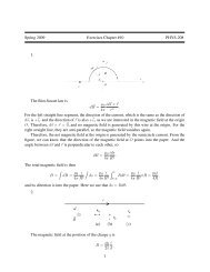
which allows us to express all dimensionful quantities in terms of a single scale whichwe choose to be mass or, equivalently, energy (since E = mc 2 has become E = m).The usual choice of energy unit is eV , the electron volt or, more often GeV = 10 9 eV orTeV = 10 12 eV . To convert the unit of energy back to a unit of length or time, we needto insert the relevant powers of c and . For example, the length scale λ associated toa mass m is the Compton wavelengthλ = mcWith this conversion factor, the electron mass m e = 10 6 eV translates to a length scaleλ e = 2 × 10 −12 m.Throughout this course we will refer to the dimension of a quantity, meaning themass dimension. If X has dimensions of (mass) d we will write [X] = d. In particular,the surviving natural quantity G has dimensions [G] = −2 and defines a mass scale,G = cM 2 p= 1M 2 p(0.2)where M p ≈ 10 19 GeV is the Planck scale. It corresponds to a length l p ≈ 10 −33 cm. ThePlanck scale is thought to be the smallest length scale that makes sense: beyond thisquantum gravity effects become important and it’s no longer clear that the conceptof spacetime makes sense. The largest length scale we can talk of is the size of thecosmological horizon, roughly 10 60 l p .ObservableUniverse~ 20 billion light yearsEarth 10 10 cmCosmologicalConstantAtoms−810 cmNuclei−1310 cmLHCPlanck Scale−3310cmlengthEnergy−3310eV−3 10eV10 1112−10eV= 1 TeV10 2819eV= 10 GeVFigure 2: Energy and Distance Scales in the UniverseSome useful scales in the universe are shown in the figure. This is a logarithmic plot,with energy increasing to the right and, correspondingly, length increasing to the left.The smallest and largest scales known are shown on the figure, together with otherrelevant energy scales. The standard model of particle physics is expected to hold up– 5 –

to about the TeV . This is precisely the regime that is currently being probed by theLarge Hadron Collider (LHC) at CERN. There is a general belief that the frameworkof quantum field theory will continue to hold to energy scales only slightly below thePlanck scale — for example, there are experimental hints that the coupling constantsof electromagnetism, and the weak and strong forces unify at around 10 18 GeV.For comparison, the rough masses of some elementary (and not so elementary) particlesare shown in the table,ParticleneutrinoselectronMuonPionsProton, NeutronTauW,Z BosonsHiggs BosonMass∼ 10 −2 eV0.5 MeV100 MeV140 MeV1 GeV2 GeV80-90 GeV120-200 GeV??– 6 –

1. Classical Field TheoryIn this first section we will discuss various aspects of classical fields. We will cover onlythe bare minimum ground necessary before turning to the quantum theory, and willreturn to classical field theory at several later stages in the course when we need tointroduce new ideas.1.1 The Dynamics of FieldsA field is a quantity defined at every point of space and time (⃗x, t). While classicalparticle mechanics deals with a finite number of generalized coordinates q a (t), indexedby a label a, in field theory we are interested in the dynamics of fieldsφ a (⃗x, t) (1.1)where both a and ⃗x are considered as labels. Thus we are dealing with a system with aninfinite number of degrees of freedom — at least one for each point ⃗x in space. Noticethat the concept of position has been relegated from a dynamical variable in particlemechanics to a mere label in field theory.An Example: The Electromagnetic FieldThe most familiar examples of fields from classical physics are the electric and magneticfields, ⃗ E(⃗x, t) and ⃗ B(⃗x, t). Both of these fields are spatial 3-vectors. In a more sophisticatedtreatement of electromagnetism, we derive these two 3-vectors from a single4-component field A µ (⃗x, t) = (φ, ⃗ A) where µ = 0, 1, 2, 3 shows that this field is a vectorin spacetime. The electric and magnetic fields are given by⃗E = −∇φ − ∂ ⃗ A∂tand ⃗ B = ∇ × ⃗ A (1.2)which ensure that two of Maxwell’s equations, ∇ · ⃗B = 0 and d ⃗ B/dt = −∇ × ⃗ E, holdimmediately as identities.The LagrangianThe dynamics of the field is governed by a Lagrangian which is a function of φ(⃗x, t),˙φ(⃗x, t) and ∇φ(⃗x, t). In all the systems we study in this course, the Lagrangian is ofthe form,∫L(t) =d 3 x L(φ a , ∂ µ φ a ) (1.3)– 7 –

where the official name for L is the Lagrangian density, although everyone simply callsit the Lagrangian. The action is,∫ t2∫ ∫S = dt d 3 x L = d 4 x L (1.4)t 1Recall that in particle mechanics L depends on q and ˙q, but not ¨q. In field theorywe similarly restrict to Lagrangians L depending on φ and ˙φ, and not ¨φ. In principle,there’s nothing to stop L depending on ∇φ, ∇ 2 φ, ∇ 3 φ, etc. However, with an eye tolater Lorentz invariance, we will only consider Lagrangians depending on ∇φ and nothigher derivatives.We can determine the equations of motion by the principle of least action. We varythe path, keeping the end points fixed and require δS = 0,∫ [ ∂LδS = d 4 x δφ a +∂L ]∂φ a ∂(∂ µ φ a ) δ(∂ µφ a )∫ [ ( )] ( )∂L ∂L∂L= d 4 x − ∂ µ δφ a + ∂ µ∂φ a ∂(∂ µ φ a ) ∂(∂ µ φ a ) δφ a (1.5)The last term is a total derivative and vanishes for any δφ a (⃗x, t) that decays at spatialinfinity and obeys δφ a (⃗x, t 1 ) = δφ a (⃗x, t 2 ) = 0. Requiring δS = 0 for all such pathsyields the Euler-Lagrange equations of motion for the fields φ a ,( ) ∂L∂ µ∂(∂ µ φ a )1.1.1 An Example: The Klein-Gordon EquationConsider the Lagrangian for a real scalar field φ(⃗x, t),− ∂L∂φ a= 0 (1.6)L = 1 2 ηµν ∂ µ φ∂ ν φ − 1 2 m2 φ 2 (1.7)= 1 2 ˙φ 2 − 1 2 (∇φ)2 − 1 2 m2 φ 2where we are using the Minkowski space metricη µν = η µν =(+1−1−1−1)(1.8)Comparing (1.7) to the usual expression for the Lagrangian L = T −V , we identify thekinetic energy of the field as∫T = d 3 x 1 ˙φ 2 (1.9)2– 8 –

and the potential energy of the field as∫V = d 3 x 1 2 (∇φ)2 + 1 2 m2 φ 2 (1.10)The first term in this expression is called the gradient energy, while the phrase “potentialenergy”, or just “potential”, is usually reserved for the last term.To determine the equations of motion arising from (1.7), we compute∂L∂φ = −m2 φ andThe Euler-Lagrange equation is thenwhich we can write in relativistic form as∂L∂(∂ µ φ) = ∂µ φ ≡ ( ˙φ, −∇φ) (1.11)¨φ − ∇ 2 φ + m 2 φ = 0 (1.12)∂ µ ∂ µ φ + m 2 φ = 0 (1.13)This is the Klein-Gordon Equation. The Laplacian in Minkowski space is sometimesdenoted by □. In this notation, the Klein-Gordon equation reads □φ + m 2 φ = 0.An obvious generalization of the Klein-Gordon equation comes from considering theLagrangian with arbitrary potential V (φ),L = 1 2 ∂ µφ∂ µ φ − V (φ) ⇒ ∂ µ ∂ µ φ + ∂V∂φ = 0 (1.14)1.1.2 Another Example: First Order LagrangiansWe could also consider a Lagrangian that is linear in time derivatives, rather thanquadratic. Take a complex scalar field ψ whose dynamics is defined by the real LagrangianL = i 2 (ψ⋆ ˙ψ − ˙ψ ⋆ ψ) − ∇ψ ⋆ · ∇ψ − mψ ⋆ ψ (1.15)We can determine the equations of motion by treating ψ and ψ ⋆ as independent objects,so that∂L∂ψ = i ⋆ 2 ˙ψ ∂L− mψ and∂ ˙ψ = − i ⋆ 2 ψ and ∂L= −∇ψ (1.16)∂∇ψ⋆ This gives us the equation of motioni ∂ψ∂t = −∇2 ψ + mψ (1.17)This looks very much like the Schrödinger equation. Except it isn’t! Or, at least, theinterpretation of this equation is very different: the field ψ is a classical field with noneof the probability interpretation of the wavefunction. We’ll come back to this point inSection 2.8.– 9 –

The initial data required on a Cauchy surface differs for the two examples above.When L ∼ ˙φ 2 , both φ and ˙φ must be specified to determine the future evolution;however when L ∼ ψ ⋆ ˙ψ, only ψ and ψ ⋆ are needed.1.1.3 A Final Example: Maxwell’s EquationsWe may derive Maxwell’s equations in the vacuum from the Lagrangian,L = − 1 2 (∂ µA ν ) (∂ µ A ν ) + 1 2 (∂ µA µ ) 2 (1.18)Notice the funny minus signs! This is to ensure that the kinetic terms for A i are positiveusing the Minkowski space metric (1.8), so L ∼ 1 A ˙22 i . The Lagrangian (1.18) has nokinetic term A ˙20 for A 0 . We will see the consequences of this in Section 6. To see thatMaxwell’s equations indeed follow from (1.18), we compute∂L∂(∂ µ A ν ) = −∂µ A ν + (∂ ρ A ρ ) η µν (1.19)from which we may derive the equations of motion,( ) ∂L∂ µ = −∂ 2 A ν + ∂ ν (∂ ρ A ρ ) = −∂ µ (∂ µ A ν − ∂ ν A µ ) ≡ −∂ µ F µν (1.20)∂(∂ µ A ν )where the field strength is defined by F µν = ∂ µ A ν − ∂ ν A µ . You can check using (1.2)that this reproduces the remaining two Maxwell’s equations in a vacuum: ∇ · ⃗E = 0and ∂ ⃗ E/∂t = ∇ × ⃗ B. Using the notation of the field strength, we may rewrite theMaxwell Lagrangian (up to an integration by parts) in the compact form1.1.4 Locality, Locality, LocalityL = − 1 4 F µνF µν (1.21)In each of the examples above, the Lagrangian is local. This means that there are noterms in the Lagrangian coupling φ(⃗x, t) directly to φ(⃗y, t) with ⃗x ≠ ⃗y. For example,there are no terms that look like∫L = d 3 xd 3 y φ(⃗x)φ(⃗y) (1.22)A priori, there’s no reason for this. After all, ⃗x is merely a label, and we’re quitehappy to couple other labels together (for example, the term ∂ 3 A 0 ∂ 0 A 3 in the MaxwellLagrangian couples the µ = 0 field to the µ = 3 field). But the closest we get for the⃗x label is a coupling between φ(⃗x) and φ(⃗x + δ⃗x) through the gradient term (∇φ) 2 .This property of locality is, as far as we know, a key feature of all theories of Nature.Indeed, one of the main reasons for introducing field theories in classical physics is toimplement locality. In this course, we will only consider local Lagrangians.– 10 –

1.2 Lorentz InvarianceThe laws of Nature are relativistic, and one of the main motivations to develop quantumfield theory is to reconcile quantum mechanics with special relativity. To this end, wewant to construct field theories in which space and time are placed on an equal footingand the theory is invariant under Lorentz transformations,x µ −→ (x ′ ) µ = Λ µ νx ν (1.23)where Λ µ ν satisfies Λ µ σ ηστ Λ ν τ = ηµν (1.24)For example, a rotation by θ about the x 3 -axis, and a boost by v < 1 along the x 1 -axisare respectively described by the Lorentz transformations⎛⎞⎛⎞1 0 0 0γ −γv 0 0Λ µ ν =0 cosθ − sin θ 0⎜⎟⎝ 0 sin θ cosθ 0 ⎠ and Λµ ν =−γv γ 0 0⎜⎟ (1.25)⎝ 0 0 1 0⎠0 0 0 10 0 0 1with γ = 1/ √ 1 − v 2 . The Lorentz transformations form a Lie group under matrixmultiplication. You’ll learn more about this in the “Symmetries and Particle Physics”course.The Lorentz transformations have a representation on the fields. The simplest exampleis the scalar field which, under the Lorentz transformation x → Λx, transformsasφ(x) → φ ′ (x) = φ(Λ −1 x) (1.26)The inverse Λ −1 appears in the argument because we are dealing with an active transformationin which the field is truly shifted. To see why this means that the inverseappears, it will suffice to consider a non-relativistic example such as a temperature field.Suppose we start with an initial field φ(⃗x) which has a hotspot at, say, ⃗x = (1, 0, 0).After a rotation ⃗x → R⃗x about the z-axis, the new field φ ′ (⃗x) will have the hotspot at⃗x = (0, 1, 0). If we want to express φ ′ (⃗x) in terms of the old field φ, we need to placeourselves at ⃗x = (0, 1, 0) and ask what the old field looked like where we’ve come fromat R −1 (0, 1, 0) = (1, 0, 0). This R −1 is the origin of the inverse transformation. (If wewere instead dealing with a passive transformation in which we relabel our choice ofcoordinates, we would have instead φ(x) → φ ′ (x) = φ(Λx)).– 11 –

The definition of a Lorentz invariant theory is that if φ(x) solves the equations ofmotion then φ(Λ −1 x) also solves the equations of motion. We can ensure that thisproperty holds by requiring that the action is Lorentz invariant. Let’s look at ourexamples:Example 1: The Klein-Gordon EquationFor a real scalar field we have φ(x) → φ ′ (x) = φ(Λ −1 x). The derivative of the scalarfield transforms as a vector, meaning(∂ µ φ)(x) → (Λ −1 ) ν µ (∂ νφ)(y)where y = Λ −1 x. This means that the derivative terms in the Lagrangian densitytransform asL deriv (x) = ∂ µ φ(x)∂ ν φ(x)η µν −→ (Λ −1 ) ρ µ (∂ ρφ)(y) (Λ −1 ) σ ν (∂ σφ)(y) η µν= (∂ ρ φ)(y) (∂ σ φ)(y) η ρσ= L deriv (y) (1.27)The potential terms transform in the same way, with φ 2 (x) → φ 2 (y). Putting this alltogether, we find that the action is indeed invariant under Lorentz transformations,∫ ∫ ∫S = d 4 x L(x) −→ d 4 x L(y) = d 4 y L(y) = S (1.28)where, in the last step, we need the fact that we don’t pick up a Jacobian factor whenwe change integration variables from ∫ d 4 x to ∫ d 4 y. This follows because det Λ = 1.(At least for Lorentz transformation connected to the identity which, for now, is all wedeal with).Example 2: First Order DynamicsIn the first-order Lagrangian (1.15), space and time are not on the same footing. (Lis linear in time derivatives, but quadratic in spatial derivatives). The theory is notLorentz invariant.In practice, it’s easy to see if the action is Lorentz invariant: just make sure allthe Lorentz indices µ = 0, 1, 2, 3 are contracted with Lorentz invariant objects, suchas the metric η µν . Other Lorentz invariant objects you can use include the totallyantisymmetric tensor ǫ µνρσ and the matrices γ µ that we will introduce when we cometo discuss spinors in Section 4.– 12 –

Example 3: Maxwell’s EquationsUnder a Lorentz transformation A µ (x) → Λ µ ν Aν (Λ −1 x). You can check that Maxwell’sLagrangian (1.21) is indeed invariant. Of course, historically electrodynamics was thefirst Lorentz invariant theory to be discovered: it was found even before the concept ofLorentz invariance.1.3 SymmetriesThe role of symmetries in field theory is possibly even more important than in particlemechanics. There are Lorentz symmetries, internal symmetries, gauge symmetries,supersymmetries.... We start here by recasting Noether’s theorem in a field theoreticframework.1.3.1 Noether’s TheoremEvery continuous symmetry of the Lagrangian gives rise to a conserved current j µ (x)such that the equations of motion implyor, in other words, ∂j 0 /∂t + ∇ ·⃗j = 0.∂ µ j µ = 0 (1.29)A Comment: A conserved current implies a conserved charge Q, defined as∫Q = d 3 x j 0R 3 (1.30)which one can immediately see by taking the time derivative,∫dQdt = d 3 x ∂j 0 ∫= − d 3 x ∇ ·⃗j = 0 (1.31)R ∂t 3 R 3assuming that ⃗j → 0 sufficiently quickly as |⃗x| → ∞. However, the existence of acurrent is a much stronger statement than the existence of a conserved charge becauseit implies that charge is conserved locally. To see this, we can define the charge in afinite volume V ,∫Q V = d 3 x j 0 (1.32)Repeating the analysis above, we find that∫∫dQ V= − d 3 x ∇ ·⃗j = −dtVVA⃗j · d ⃗ S (1.33)– 13 –

where A is the area bounding V and we have used Stokes’ theorem. This equationmeans that any charge leaving V must be accounted for by a flow of the current 3-vector ⃗j out of the volume. This kind of local conservation of charge holds in any localfield theory.Proof of Noether’s Theorem: We’ll prove the theorem by working infinitesimally.We may always do this if we have a continuous symmetry. We say that the transformationδφ a (x) = X a (φ) (1.34)is a symmetry if the Lagrangian changes by a total derivative,δL = ∂ µ F µ (1.35)for some set of functions F µ (φ). To derive Noether’s theorem, we first consider makingan arbitrary transformation of the fields δφ a . ThenδL = ∂L δφ a +∂L∂φ a ∂(∂ µ φ a ) ∂ µ(δφ a )[ ] ( )∂L ∂L∂L= − ∂ µ δφ a + ∂ µ∂φ a ∂(∂ µ φ a ) ∂(∂ µ φ a ) δφ a(1.36)When the equations of motion are satisfied, the term in square brackets vanishes. Sowe’re left with( ) ∂LδL = ∂ µ∂(∂ µ φ a ) δφ a(1.37)But for the symmetry transformation δφ a = X a (φ), we have by definition δL = ∂ µ F µ .Equating this expression with (1.37) gives us the result∂ µ j µ = 0 with j µ = ∂L∂(∂ µ φ a ) X a(φ) − F µ (φ) (1.38)1.3.2 An Example: Translations and the Energy-Momentum TensorRecall that in classical particle mechanics, invariance under spatial translations givesrise to the conservation of momentum, while invariance under time translations isresponsible for the conservation of energy. We will now see something similar in fieldtheories. Consider the infinitesimal translationx ν → x ν − ǫ ν ⇒ φ a (x) → φ a (x) + ǫ ν ∂ ν φ a (x) (1.39)– 14 –

(where the sign in the field transformation is plus, instead of minus, because we’re doingan active, as opposed to passive, transformation). Similarly, the Lagrangian transformsasL(x) → L(x) + ǫ ν ∂ ν L(x) (1.40)(This is the correct transformation for a Lagrangian that has no explicit x dependence,but only depends on x through the fields φ a (x). All theories that we consider in thiscourse will have this property). Since the change in the Lagrangian is a total derivative,we may invoke Noether’s theorem which gives us four conserved currents (j µ ) ν , one foreach of the translations ǫ ν with ν = 0, 1, 2, 3,T µ ν(j µ ) ν = ∂L∂(∂ µ φ a ) ∂ νφ a − δ µ ν L ≡ T µ ν (1.41)is called the energy-momentum tensor. It satisfies∂ µ T µ ν = 0 (1.42)The four conserved quantities are given by∫∫E = d 3 x T 00 and P i =d 3 x T 0i (1.43)where E is the total energy of the field configuration, while P i is the total momentumof the field configuration.An Example of the Energy-Momentum TensorConsider the simplest scalar field theory with Lagrangian (1.7). From the above discussion,we can computeT µν = ∂ µ φ ∂ ν φ − η µν L (1.44)One can verify using the equation of motion for φ that this expression indeed satisfies∂ µ T µν = 0. For this example, the conserved energy and momentum are given by∫E = d 3 x 1 ˙φ 2 + 1 2 2 (∇φ)2 + 1 2 m2 φ 2 (1.45)∫P i = d 3 x ˙φ∂ i φ (1.46)Notice that for this example, T µν came out symmetric, so that T µν = T νµ . Thiswon’t always be the case. Nevertheless, there is typically a way to massage the energymomentum tensor of any theory into a symmetric form by adding an extra termΘ µν = T µν + ∂ ρ Γ ρµν (1.47)– 15 –

where Γ ρµν is some function of the fields that is anti-symmetric in the first two indices soΓ ρµν = −Γ µρν . This guarantees that ∂ µ ∂ ρ Γ ρµν = 0 so that the new energy-momentumtensor is also a conserved current.A Cute TrickOne reason that you may want a symmetric energy-momentum tensor is to make contactwith general relativity: such an object sits on the right-hand side of Einstein’sfield equations. In fact this observation provides a quick and easy way to determine asymmetric energy-momentum tensor. Firstly consider coupling the theory to a curvedbackground spacetime, introducing an arbitrary metric g µν (x) in place of η µν , and replacingthe kinetic terms with suitable covariant derivatives using “minimal coupling”.Then a symmetric energy momentum tensor in the flat space theory is given byΘ µν = − 2 √ −g∂( √ −gL)∂g µν∣ ∣∣∣gµν=η µν(1.48)It should be noted however that this trick requires a little more care when workingwith spinors.1.3.3 Another Example: Lorentz Transformations and Angular MomentumIn classical particle mechanics, rotational invariance gave rise to conservation of angularmomentum. What is the analogy in field theory? Moreover, we now have furtherLorentz transformations, namely boosts. What conserved quantity do they correspondto? To answer these questions, we first need the infinitesimal form of the LorentztransformationsΛ µ ν = δ µ ν + ω µ ν (1.49)where ω µ ν is infinitesimal. The condition (1.24) for Λ to be a Lorentz transformationbecomes(δ µ σ + ω µ σ)(δ ν τ + ω ν τ) η στ = η µν⇒ ω µν + ω νµ = 0 (1.50)So the infinitesimal form ω µν of the Lorentz transformation must be an anti-symmetricmatrix. As a check, the number of different 4×4 anti-symmetric matrices is 4×3/2 = 6,which agrees with the number of different Lorentz transformations (3 rotations + 3boosts). Now the transformation on a scalar field is given byφ(x) → φ ′ (x) = φ(Λ −1 x)= φ(x µ − ω µ ν xν )= φ(x µ ) − ω µ ν xν ∂ µ φ(x) (1.51)– 16 –

from which we see thatδφ = −ω µ ν xν ∂ µ φ (1.52)By the same argument, the Lagrangian density transforms asδL = −ω µ νx ν ∂ µ L = −∂ µ (ω µ νx ν L) (1.53)where the last equality follows because ω µ µ = 0 due to anti-symmetry. Once again,the Lagrangian changes by a total derivative so we may apply Noether’s theorem (nowwith F µ = −ω µ ν xν L) to find the conserved currentj µ = −∂L∂(∂ µ φ) ωρ νx ν ∂ ρ φ + ω µ ν x ν L[ ]∂L= −ω ρ ν∂(∂ µ φ) xν ∂ ρ φ − δ µ ρ x ν L = −ω ρ ν T µ ρx ν (1.54)Unlike in the previous example, I’ve left the infinitesimal choice of ω µ ν in the expressionfor this current. But really, we should strip it out to give six different currents, i.e. onefor each choice of ω µ ν . We can write them as(J µ ) ρσ = x ρ T µσ − x σ T µρ (1.55)which satisfy ∂ µ (J µ ) ρσ = 0 and give rise to 6 conserved charges. For ρ, σ = 1, 2, 3,the Lorentz transformation is a rotation and the three conserved charges give the totalangular momentum of the field.∫Q ij = d 3 x (x i T 0j − x j T 0i ) (1.56)But what about the boosts? In this case, the conserved charges are∫Q 0i = d 3 x (x 0 T 0i − x i T 00 ) (1.57)The fact that these are conserved tells us that∫ ∫0 = dQ0i= d 3 x T 0i + t d 3 0i∂Tx − d ∫d 3 x x i T 00dt∂t dt= P i + t dP idt − d ∫d 3 x x i T 00 (1.58)dtBut we know that P i is conserved, so dP i /dt = 0, leaving us with the following consequenceof invariance under boosts:∫dd 3 x x i T 00 = constant (1.59)dtThis is the statement that the center of energy of the field travels with a constantvelocity. It’s kind of like a field theoretic version of Newton’s first law but, rathersurprisingly, appearing here as a conservation law.– 17 –

1.3.4 Internal SymmetriesThe above two examples involved transformations of spacetime, as well as transformationsof the field. An internal symmetry is one that only involves a transformation ofthe fields and acts the same at every point in spacetime. The simplest example occursfor a complex scalar field ψ(x) = (φ 1 (x)+iφ 2 (x))/ √ 2. We can build a real LagrangianbyL = ∂ µ ψ ⋆ ∂ µ ψ − V (|ψ| 2 ) (1.60)where the potential is a general polynomial in |ψ| 2 = ψ ⋆ ψ. To find the equations ofmotion, we could expand ψ in terms of φ 1 and φ 2 and work as before. However, it’seasier (and equivalent) to treat ψ and ψ ⋆ as independent variables and vary the actionwith respect to both of them. For example, varying with respect to ψ ⋆ leads to theequation of motion∂ µ ∂ µ ψ + ∂V (ψ⋆ ψ)∂ψ ⋆ = 0 (1.61)The Lagrangian has a continuous symmetry which rotates φ 1 and φ 2 or, equivalently,rotates the phase of ψ:ψ → e iα ψ or δψ = iαψ (1.62)where the latter equation holds with α infinitesimal. The Lagrangian remains invariantunder this change: δL = 0. The associated conserved current isj µ = i(∂ µ ψ ⋆ )ψ − iψ ⋆ (∂ µ ψ) (1.63)We will later see that the conserved charges arising from currents of this type havethe interpretation of electric charge or particle number (for example, baryon or leptonnumber).Non-Abelian Internal SymmetriesConsider a theory involving N scalar fields φ a , all with the same mass and the Lagrangian(L = 1 N∑∂ µ φ a ∂ µ φ a − 1 N∑N 2m 2 φ 2 a22− g ∑φa) 2 (1.64)a=1a=1In this case the Lagrangian is invariant under the non-Abelian symmetry group G =SO(N). (Actually O(N) in this case). One can construct theories from complex fieldsin a similar manner that are invariant under an SU(N) symmetry group. Non-Abeliansymmetries of this type are often referred to as global symmetries to distinguish themfrom the “local gauge” symmetries that you will meet later. Isospin is an example ofsuch a symmetry, albeit realized only approximately in Nature.a=1– 18 –

Another Cute TrickThere is a quick method to determine the conserved current associated to an internalsymmetry δφ = αφ for which the Lagrangian is invariant. Here, α is a constant realnumber. (We may generalize the discussion easily to a non-Abelian internal symmetryfor which α becomes a matrix). Now consider performing the transformation but whereα depends on spacetime: α = α(x). The action is no longer invariant. However, thechange must be of the formδL = (∂ µ α) h µ (φ) (1.65)since we know that δL = 0 when α is constant. The change in the action is therefore∫ ∫δS = d 4 x δL = − d 4 x α(x) ∂ µ h µ (1.66)which means that when the equations of motion are satisfied (so δS = 0 for all variations,including δφ = α(x)φ) we have∂ µ h µ = 0 (1.67)We see that we can identify the function h µ = j µ as the conserved current. This wayof viewing things emphasizes that it is the derivative terms, not the potential terms,in the action that contribute to the current. (The potential terms are invariant evenwhen α = α(x)).1.4 The Hamiltonian FormalismThe link between the Lagrangian formalism and the quantum theory goes via the pathintegral. In this course we will not discuss path integral methods, and focus insteadon canonical quantization. For this we need the Hamiltonian formalism of field theory.We start by defining the momentum π a (x) conjugate to φ a (x),π a (x) = ∂L∂ ˙φ a(1.68)The conjugate momentum π a (x) is a function of x, just like the field φ a (x) itself. Itis not to be confused with the total momentum P i defined in (1.43) which is a singlenumber characterizing the whole field configuration. The Hamiltonian density is givenbyH = π a (x) ˙φ a (x) − L(x) (1.69)where, as in classical mechanics, we eliminate ˙φ a (x) in favour of π a (x) everywhere inH. The Hamiltonian is then simply∫H = d 3 x H (1.70)– 19 –

An Example: A Real Scalar FieldFor the LagrangianL = 1 2 ˙φ 2 − 1 2 (∇φ)2 − V (φ) (1.71)the momentum is given by π = ˙φ, which gives us the Hamiltonian,∫H = d 3 x 1 2 π2 + 1 2 (∇φ)2 + V (φ) (1.72)Notice that the Hamiltonian agrees with the definition of the total energy (1.45) thatwe get from applying Noether’s theorem for time translation invariance.In the Lagrangian formalism, Lorentz invariance is clear for all to see since the actionis invariant under Lorentz transformations. In contrast, the Hamiltonian formalism isnot manifestly Lorentz invariant: we have picked a preferred time. For example, theequations of motion for φ(x) = φ(⃗x, t) arise from Hamilton’s equations,˙φ(⃗x, t) =∂H∂π(⃗x, t)and ˙π(⃗x, t) = − ∂H∂φ(⃗x, t)(1.73)which, unlike the Euler-Lagrange equations (1.6), do not look Lorentz invariant. Nevertheless,even though the Hamiltonian framework doesn’t look Lorentz invariant, thephysics must remain unchanged. If we start from a relativistic theory, all final answersmust be Lorentz invariant even if it’s not manifest at intermediate steps. We will pauseat several points along the quantum route to check that this is indeed the case.– 20 –

2. Free Fields“The career of a young theoretical physicist consists of treating the harmonicoscillator in ever-increasing levels of abstraction.”Sidney Coleman2.1 Canonical QuantizationIn quantum mechanics, canonical quantization is a recipe that takes us from the Hamiltonianformalism of classical dynamics to the quantum theory. The recipe tells us totake the generalized coordinates q a and their conjugate momenta p a and promote themto operators. The Poisson bracket structure of classical mechanics morphs into thestructure of commutation relations between operators, so that, in units with = 1,[q a , q b ] = [p a , p b ] = 0[q a , p b ] = i δ b a (2.1)In field theory we do the same, now for the field φ a (⃗x) and its momentum conjugateπ b (⃗x). Thus a quantum field is an operator valued function of space obeying the commutationrelations[φ a (⃗x), φ b (⃗y)] = [π a (⃗x), π b (⃗y)] = 0[φ a (⃗x), π b (⃗y)] = iδ (3) (⃗x − ⃗y) δ b a (2.2)Note that we’ve lost all track of Lorentz invariance since we have separated space ⃗xand time t. We are working in the Schrödinger picture so that the operators φ a (⃗x) andπ a (⃗x) do not depend on time at all — only on space. All time dependence sits in thestates |ψ〉 which evolve by the usual Schrödinger equationi d|ψ〉dt= H |ψ〉 (2.3)We aren’t doing anything different from usual quantum mechanics; we’re merely applyingthe old formalism to fields. Be warned however that the notation |ψ〉 for the stateis deceptively simple: if you were to write the wavefunction in quantum field theory, itwould be a functional, that is a function of every possible configuration of the field φ.The typical information we want to know about a quantum theory is the spectrum ofthe Hamiltonian H. In quantum field theories, this is usually very hard. One reason forthis is that we have an infinite number of degrees of freedom — at least one for everypoint ⃗x in space. However, for certain theories — known as free theories — we can finda way to write the dynamics such that each degree of freedom evolves independently– 21 –

from all the others. Free field theories typically have Lagrangians which are quadraticin the fields, so that the equations of motion are linear. For example, the simplestrelativistic free theory is the classical Klein-Gordon (KG) equation for a real scalarfield φ(⃗x, t),∂ µ ∂ µ φ + m 2 φ = 0 (2.4)To exhibit the coordinates in which the degrees of freedom decouple from each other,we need only take the Fourier transform,∫d 3 pφ(⃗x, t) = ei⃗p·⃗x φ(⃗p, t) (2.5)(2π) 3Then φ(⃗p, t) satisfies( )∂2∂t + (⃗p 2 + m 2 ) φ(⃗p, t) = 0 (2.6)2Thus, for each value of ⃗p, φ(⃗p, t) solves the equation of a harmonic oscillator vibratingat frequencyω ⃗p = + √ ⃗p 2 + m 2 (2.7)We learn that the most general solution to the KG equation is a linear superposition ofsimple harmonic oscillators, each vibrating at a different frequency with a different amplitude.To quantize φ(⃗x, t) we must simply quantize this infinite number of harmonicoscillators. Let’s recall how to do this.2.1.1 The Simple Harmonic OscillatorConsider the quantum mechanical HamiltonianH = 1 2 p2 + 1 2 ω2 q 2 (2.8)with the canonical commutation relations [q, p] = i. To find the spectrum we definethe creation and annihilation operators (also known as raising/lowering operators, orsometimes ladder operators)a =√ ω2 q +which can be easily inverted to give√ i √ ωp , a † =2ω 2 q −i √2ωp (2.9)q = 1 √2ω(a + a † ) , p = −i√ ω2 (a − a† ) (2.10)– 22 –

Substituting into the above expressions we findwhile the Hamiltonian is given by[a, a † ] = 1 (2.11)H = 1 2 ω(aa† + a † a)= ω(a † a + 1 2 ) (2.12)One can easily confirm that the commutators between the Hamiltonian and the creationand annihilation operators are given by[H, a † ] = ωa † and [H, a] = −ωa (2.13)These relations ensure that a and a † take us between energy eigenstates. Let |E〉 bean eigenstate with energy E, so that H |E〉 = E |E〉. Then we can construct moreeigenstates by acting with a and a † ,Ha † |E〉 = (E + ω)a † |E〉 , Ha |E〉 = (E − ω)a |E〉 (2.14)So we find that the system has a ladder of states with energies. . .,E − ω, E, E + ω, E + 2ω, . . . (2.15)If the energy is bounded below, there must be a ground state |0〉 which satisfies a |0〉 = 0.This has ground state energy (also known as zero point energy),Excited states then arise from repeated application of a † ,H |0〉 = 1 ω |0〉 (2.16)2|n〉 = (a † ) n |0〉 with H |n〉 = (n + 1 )ω |n〉 (2.17)2where I’ve ignored the normalization of these states so, 〈n| n〉 ≠ 1.2.2 The Free Scalar FieldWe now apply the quantization of the harmonic oscillator to the free scalar field. Wewrite φ and π as a linear sum of an infinite number of creation and annihilation operatorsa † ⃗p and a ⃗p, indexed by the 3-momentum ⃗p,∫φ(⃗x) =∫π(⃗x) =d 3 p 1[]√ a(2π) 3 ⃗p e i⃗p·⃗x + a † e−i⃗p·⃗x ⃗p 2ω⃗p√d 3 p ω⃗p(2π) 3(−i) 2[a ⃗p e i⃗p·⃗x − a † ⃗p e−i⃗p·⃗x ](2.18)(2.19)– 23 –

Claim: The commutation relations for φ and π are equivalent to the following commutationrelations for a ⃗p and a † ⃗p[φ(⃗x), φ(⃗y)] = [π(⃗x), π(⃗y)] = 0[φ(⃗x), π(⃗y)] = iδ (3) (⃗x − ⃗y)⇔[a ⃗p, a ⃗q ] = [a † ⃗p , a† ⃗q ] = 0[a ⃗p, a † ⃗q ] = (2π)3 δ (3) (⃗p − ⃗q)(2.20)Proof: We’ll show this just one way. Assume that [a ⃗p, a † ⃗q ] = (2π)3 δ (3) (⃗p − ⃗q). Then∫ d 3 p d 3 √q (−i) ω⃗q()[φ(⃗x), π(⃗y)] =−[a(2π) 6 2 ω ⃗p , a † ⃗q ] ei⃗p·⃗x−i⃗q·⃗y + [a † ⃗p , a ⃗q] e −i⃗p·⃗x+i⃗q·⃗y⃗p∫d 3 p (−i) (=−e i⃗p·(⃗x−⃗y) − e i⃗p·(⃗y−⃗x)) (2.21)(2π) 3 2The Hamiltonian= iδ (3) (⃗x − ⃗y) □Let’s now compute the Hamiltonian in terms of a ⃗pand a † ⃗p. We haveH = 1 ∫d 3 x π 2 + (∇φ) 2 + m 2 φ 22= 1 ∫ [ d 3 x d 3 p d 3 √q ω⃗p ω ⃗q− (a2 (2π) 6 2 ⃗p e i⃗p·⃗x − a † e−i⃗p·⃗x ⃗p)(a ⃗q e i⃗q·⃗x − a † e−i⃗q·⃗x ⃗q)+ 12 √ (i⃗p aω ⃗p ω ⃗p e i⃗p·⃗x − i⃗p a † e−i⃗p·⃗x ⃗p) · (i⃗q a ⃗q e i⃗q·⃗x − i⃗q a † e−i⃗q·⃗x ⃗q)⃗q]+ m22 √ (aω ⃗p ω ⃗p e i⃗p·⃗x + a † e−i⃗p·⃗x ⃗p)(a ⃗q e i⃗q·⃗x + a † e−i⃗q·⃗x ⃗q)⃗q= 1 ∫d 3 p 1[](−ω4 (2π) 3 ⃗p 2 ω + ⃗p 2 + m 2 )(a ⃗p a −⃗p + a † ⃗p a† −⃗p ) + (ω2 ⃗p + ⃗p 2 + m 2 )(a ⃗p a † ⃗p + a† ⃗p a ⃗p )⃗pwhere in the second line we’ve used the expressions for φ and π given in (2.18) and(2.19); to get to the third line we’ve integrated over d 3 x to get delta-functions δ (3) (⃗p±⃗q)which, in turn, allow us to perform the d 3 q integral. Now using the expression for thefrequency ω 2 ⃗p = ⃗p 2 + m 2 , the first term vanishes and we’re left withH = 1 2∫=∫d 3 p(2π) ω 3 ⃗pd 3 p(2π) 3 ω ⃗p[ ]a ⃗p a † ⃗p + a† ⃗p a ⃗p[]a † ⃗p a ⃗p + 1 2 (2π)3 δ (3) (0)(2.22)– 24 –

Hmmmm. We’ve found a delta-function, evaluated at zero where it has its infinitespike. Moreover, the integral over ω ⃗p diverges at large p. What to do? Let’s start bylooking at the ground state where this infinity first becomes apparent.2.3 The VacuumFollowing our procedure for the harmonic oscillator, let’s define the vacuum |0〉 byinsisting that it is annihilated by all a ⃗p,a ⃗p |0〉 = 0 ∀ ⃗p (2.23)With this definition, the energy E 0 of the ground state comes from the second term in(2.22),[∫H |0〉 ≡ E 0 |0〉 = d 3 p 1 ]2 ω ⃗p δ (3) (0) | 0〉 = ∞ |0〉 (2.24)The subject of quantum field theory is rife with infinities. Each tells us somethingimportant, usually that we’re doing something wrong, or asking the wrong question.Let’s take some time to explore where this infinity comes from and how we should dealwith it.In fact there are two different ∞’s lurking in the expression (2.24). The first arisesbecause space is infinitely large. (Infinities of this type are often referred to as infra-reddivergences although in this case the ∞ is so simple that it barely deserves this name).To extract out this infinity, let’s consider putting the theory in a box with sides oflength L. We impose periodic boundary conditions on the field. Then, taking the limitwhere L → ∞, we get∫ L/2(2π) 3 δ (3) (0) = lim d 3 x e i⃗x·⃗p∣ ∫ L/2∣L→∞ ⃗p=0= lim d 3 x = V (2.25)−L/2L→∞−L/2where V is the volume of the box. So the δ(0) divergence arises because we’re computingthe total energy, rather than the energy density E 0 . To find E 0 we can simply divide bythe volume,E 0 = E ∫0V = d 3 p 1(2π) 3 2 ω ⃗p (2.26)which is still infinite. We recognize it as the sum of ground state energies for eachharmonic oscillator. But E 0 → ∞ due to the |⃗p| → ∞ limit of the integral. This isa high frequency — or short distance — infinity known as an ultra-violet divergence.This divergence arises because of our hubris. We’ve assumed that our theory is validto arbitrarily short distance scales, corresponding to arbitrarily high energies. This isclearly absurd. The integral should be cut-off at high momentum in order to reflectthe fact that our theory is likely to break down in some way.– 25 –

We can deal with the infinity in (2.24) in a more practical way. In physics we’reonly interested in energy differences. There’s no way to measure E 0 directly, so we cansimply redefine the Hamiltonian by subtracting off this infinity,∫H =d 3 p(2π) 3 ω ⃗p a † ⃗p a ⃗p (2.27)so that, with this new definition, H |0〉 = 0. In fact, the difference between this Hamiltonianand the previous one is merely an ordering ambiguity in moving from the classicaltheory to the quantum theory. For example, if we defined the Hamiltonian of the harmonicoscillator to be H = (1/2)(ωq −ip)(ωq +ip), which is classically the same as ouroriginal choice, then upon quantization it would naturally give H = ωa † a as in (2.27).This type of ordering ambiguity arises a lot in field theories. We’ll come across a numberof ways of dealing with it. The method that we’ve used above is called normal ordering.Definition: We write the normal ordered string of operators φ 1 (⃗x 1 ) . . .φ n (⃗x n ) as: φ 1 (⃗x 1 ) . . .φ n (⃗x n ) : (2.28)It is defined to be the usual product with all annihilation operators a ⃗pplaced to theright. So, for the Hamiltonian, we could write (2.27) as∫d 3 p: H :=(2π) ω 3 ⃗p a † ⃗p a ⃗p (2.29)In the remainder of this section, we will normal order all operators in this manner.2.3.1 The Cosmological ConstantAbove I wrote “there’s no way to measure E 0 directly”. There is a BIG caveat here:gravity is supposed to see everything! The sum of all the zero point energies shouldcontribute to the stress-energy tensor that appears on the right-hand side of Einstein’sequations. We expect them to appear as a cosmological constant Λ = E 0 /V ,R µν − 1 2 g µν = −8πGT µν + Λg µν (2.30)Current observation suggests that 70% of the energy density in the universe has theproperties of a cosmological constant with Λ ∼ (10 −3 eV ) 4 . This is much smaller thanother scales in particle physics. In particular, the Standard Model is valid at least upto 10 12 eV . Why don’t the zero point energies of these fields contribute to Λ? Or, ifthey do, what cancels them to such high accuracy? This is the cosmological constantproblem. No one knows the answer!– 26 –

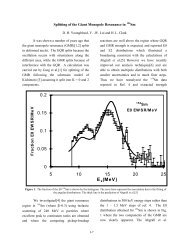
2.3.2 The Casimir Effect“I mentioned my results to Niels Bohr, during a walk. That is nice, hesaid, that is something new... and he mumbled something about zero-pointenergy.”Hendrik CasimirUsing the normal ordering prescription we can happily set E 0 = 0, while chantingthe mantra that only energy differences can be measured. But we should be careful, forthere is a situation where differences in the energy of vacuum fluctuations themselvescan be measured.To regulate the infra-red divergences, we’ll make the x 1 direction periodic, with sizeL, and impose periodic boundary conditions such thatφ(⃗x) = φ(⃗x + L⃗n) (2.31)with ⃗n = (1, 0, 0). We’ll leave y and z alone, but rememberthat we should compute all physical quantities per unit areaA. We insert two reflecting plates, separated by a distanced ≪ L in the x 1 direction. The plates are such that theyimpose φ(x) = 0 at the position of the plates. The presence ofthese plates affects the Fourier decomposition of the field and,in particular, means that the momentum of the field inside theplates is quantized as( nπ)⃗p =d , p y, p z n ∈ Z + (2.32)LFigure 3:dFor a massless scalar field, the ground state energy between the plates isE(d)A∞ = ∑∫ dpy dp z 1 (nπ ) 2+ p2(2π) 2√ 2 d y + p 2 z (2.33)n=1while the energy outside the plates is E(L − d). The total energy is thereforeE = E(d) + E(L − d) (2.34)which – at least naively – depends on d. If this naive guess is true, it would meanthat there is a force on the plates due to the fluctuations of the vacuum. This is theCasimir force, first predicted in 1948 and observed 10 years later. In the real world, theeffect is due to the vacuum fluctuations of the electromagnetic field, with the boundaryconditions imposed by conducting plates. Here we model this effect with a scalar.– 27 –

But there’s a problem. E is infinite! What to do? The problem comes from thearbitrarily high momentum modes. We could regulate this in a number of differentways. Physically one could argue that any real plate cannot reflect waves of arbitrarilyhigh frequency: at some point, things begin to leak. Mathematically, we want to finda way to neglect modes of momentum p ≫ a −1 for some distance scale a ≪ d, knownas the ultra-violet (UV) cut-off. One way to do this is to change the integral (2.33) to,E(d)A∞ = ∑∫ (√ )dpy dp z 1 (nπ ) 2+ p2(2π) 2 2 d y + p 2 zn=1e −a q(nπd ) 2 +p 2 y+p 2 z(2.35)which has the property that as a → 0, we regain the full, infinite, expression (2.33).However (2.35) is finite, and gives us something we can easily work with. Of course,we made it finite in a rather ad-hoc manner and we better make sure that any physicalquantity we calculate doesn’t depend on the UV cut-off a, otherwise it’s not somethingwe can really trust.The integral (2.35) is do-able, but a little complicated. It’s a lot simpler if we lookat the problem in d = 1 + 1 dimensions, rather than d = 3 + 1 dimensions. We’ll findthat all the same physics is at play. Now the energy is given byE 1+1 (d) = π ∞∑n (2.36)2dWe now regulate this sum by introducing the UV cutoff a introduced above. Thisrenders the expression finite, allowing us to start manipulating it thus,E 1+1 (d) → π ∞∑n e −anπ/d2dn=1= − 1 ∂2 ∂an=1∞∑n=1e −anπ/d= − 1 ∂ 12 ∂a 1 − e −aπ/d= π e aπ/d2d (e aπ/d − 1) 2= d2πa − π2 24d + O(a2 ) (2.37)where, in the last line, we’ve used the fact that a ≪ d. We can now compute the fullenergy,E 1+1 = E 1+1 (d) + E 1+1 (L − d) =L2πa − π ( 1 2 24 d + 1 )+ O(a 2 ) (2.38)L − d– 28 –

This is still infinite in the limit a → 0, which is to be expected. However, the force isgiven by∂E 1+1∂d= π24d 2 + . . . (2.39)where the . . . include terms of size d/L and a/d. The key point is that as we removeboth the regulators, and take a → 0 and L → ∞, the force between the plates remainsfinite. This is the Casimir force 2 .If we ploughed through the analogous calculation in d = 3 + 1 dimensions, andperformed the integral (2.35), we would find the result1 ∂EA ∂d =π2480d 4 (2.40)The true Casimir force is twice as large as this, due to the two polarization states ofthe photon.2.4 ParticlesHaving dealt with the vacuum, we can now turn to the excitations of the field. It’seasy to verify that[H, a † ⃗p ] = ω ⃗p a † ⃗pand [H, a ⃗p ] = −ω ⃗p a ⃗p (2.41)which means that, just as for the harmonic oscillator, we can construct energy eigenstatesby acting on the vacuum |0〉 with a † ⃗p . LetThis state has energy|⃗p〉 = a † ⃗p|0〉 (2.42)H |⃗p〉 = ω ⃗p |⃗p〉 with ω 2 ⃗p = ⃗p 2 + m 2 (2.43)But we recognize this as the relativistic dispersion relation for a particle of mass m and3-momentum ⃗p,E 2 ⃗p = ⃗p 2 + m 2 (2.44)2 The number 24 that appears in the denominator of the one-dimensional Casimir force plays a morefamous role in string theory: the same calculation in that context is the reason the bosonic string livesin 26 = 24 + 2 spacetime dimensions. (The +2 comes from the fact the string itself is extended in onespace and one time dimension). You will need to attend next term’s “String Theory” course to seewhat on earth this has to do with the Casimir force.– 29 –

We interpret the state |⃗p〉 as the momentum eigenstate of a single particle of mass m.To stress this, from now on we’ll write E ⃗p everywhere instead of ω ⃗p . Let’s check thisparticle interpretation by studying the other quantum numbers of |⃗p〉. We may takethe classical total momentum P ⃗ given in (1.46) and turn it into an operator. Afternormal ordering, it becomes∫⃗P = −∫d 3 x π ∇φ ⃗ =d 3 p(2π) 3 ⃗p a† ⃗p a ⃗p (2.45)Acting on our state |⃗p〉 with ⃗ P, we learn that it is indeed an eigenstate,⃗P |⃗p〉 = ⃗p |⃗p〉 (2.46)telling us that the state |⃗p〉 has momentum ⃗p. Another property of |⃗p〉 that we canstudy is its angular momentum. Once again, we may take the classical expression forthe total angular momentum of the field (1.55) and turn it into an operator,J i = ǫ ijk ∫d 3 x (J 0 ) jk (2.47)It’s not hard to show that acting on the one-particle state with zero momentum,J i |⃗p = 0〉 = 0, which we interpret as telling us that the particle carries no internalangular momentum. In other words, quantizing a scalar field gives rise to a spin 0particle.Multi-Particle States, Bosonic Statistics and Fock SpaceWe can create multi-particle states by acting multiple times with a † ’s. We interpretthe state in which n a † ’s act on the vacuum as an n-particle state,|⃗p 1 , . . .,⃗p n 〉 = a † ⃗p 1. . .a † ⃗p n|0〉 (2.48)Because all the a † ’s commute among themselves, the state is symmetric under exchangeof any two particles. For example,This means that the particles are bosons.|⃗p,⃗q〉 = |⃗q, ⃗p〉 (2.49)The full Hilbert space of our theory is spanned by acting on the vacuum with allpossible combinations of a † ’s,|0〉 , a † ⃗p |0〉 , a† ⃗p a† ⃗q |0〉 , a† ⃗p a† ⃗q a† ⃗r|0〉... (2.50)– 30 –

This space is known as a Fock space. The Fock space is simply the sum of the n-particleHilbert spaces, for all n ≥ 0. There is a useful operator which counts the number ofparticles in a given state in the Fock space. It is called the number operator N∫N =d 3 p(2π) 3 a† ⃗p a ⃗p (2.51)and satisfies N |⃗p 1 , . . .,⃗p n 〉 = n |⃗p 1 , . . .,⃗p n 〉. The number operator commutes with theHamiltonian, [N, H] = 0, ensuring that particle number is conserved. This means thatwe can place ourselves in the n-particle sector, and stay there. This is a property offree theories, but will no longer be true when we consider interactions: interactionscreate and destroy particles, taking us between the different sectors in the Fock space.Operator Valued DistributionsAlthough we’re referring to the states |⃗p〉 as “particles”, they’re not localized in spacein any way — they are momentum eigenstates. Recall that in quantum mechanics theposition and momentum eigenstates are not good elements of the Hilbert space sincethey are not normalizable (they normalize to delta-functions). Similarly, in quantumfield theory neither the operators φ(⃗x), nor a ⃗pare good operators acting on the Fockspace. This is because they don’t produce normalizable states. For example,〈0|a ⃗p a † ⃗p |0〉 = 〈⃗p| ⃗p〉 = (2π)3 δ(0) and 〈0|φ(⃗x) φ(⃗x) |0〉 = 〈⃗x|⃗x〉 = δ(0) (2.52)They are operator valued distributions, rather than functions. This means that althoughφ(⃗x) has a well defined vacuum expectation value, 〈0|φ(⃗x) |0〉 = 0, the fluctuationsof the operator at a fixed point are infinite, 〈0|φ(⃗x)φ(⃗x) |0〉 = ∞. We canconstruct well defined operators by smearing these distributions over space. For example,we can create a wavepacket∫|ϕ〉 =d 3 p(2π) 3 e−i⃗p·⃗x ϕ(⃗p) |⃗p〉 (2.53)which is partially localized in both position and momentum space. (A typical statemight be described by the Gaussian ϕ(⃗p) = exp(−⃗p 2 /2m 2 )).2.4.1 Relativistic NormalizationWe have defined the vacuum |0〉 which we normalize as 〈0| 0〉 = 1. The one-particlestates |⃗p〉 = a † ⃗p |0〉 then satisfy 〈⃗p|⃗q〉 = (2π) 3 δ (3) (⃗p − ⃗q) (2.54)– 31 –

But is this Lorentz invariant? It’s not obvious because we only have 3-vectors. Whatcould go wrong? Suppose we have a Lorentz transformationp µ → (p ′ ) µ = Λ µ ν p ν (2.55)such that the 3-vector transforms as ⃗p → ⃗p ′ . In the quantum theory, it would bepreferable if the two states are related by a unitary transformation,|⃗p〉 → |⃗p ′ 〉 = U(Λ) |⃗p〉 (2.56)This would mean that the normalizations of |⃗p〉 and |⃗p ′ 〉 are the same whenever ⃗p and⃗p ′ are related by a Lorentz transformation. But we haven’t been at all careful withnormalizations. In general, we could get|⃗p〉 → λ(⃗p, ⃗p ′ ) |⃗p ′ 〉 (2.57)for some unknown function λ(⃗p, ⃗p ′ ). How do we figure this out? The trick is to look atan object which we know is Lorentz invariant. One such object is the identity operatoron one-particle states (which is really the projection operator onto one-particle states).With the normalization (2.54) we know this is given by∫1 =d 3 p|⃗p〉 〈⃗p| (2.58)(2π)3This operator is Lorentz invariant, but it consists of two terms: the measure ∫ d 3 p andthe projector |⃗p〉〈⃗p|. Are these individually Lorentz invariant? In fact the answer is no.Claim The Lorentz invariant measure is,∫ d 3 p2E ⃗p(2.59)Proof: ∫ d 4 p is obviously Lorentz invariant. And the relativistic dispersion relationfor a massive particle,p µ p µ = m 2 ⇒ p 2 0 = E2 ⃗p = ⃗p 2 + m 2 (2.60)is also Lorentz invariant. Solving for p 0 , there are two branches of solutions: p 0 = ±E ⃗p .But the choice of branch is another Lorentz invariant concept. So piecing everythingtogether, the following combination must be Lorentz invariant,∫∫ ∣ d 4 p δ(p 2 0 − ⃗p 2 − m 2 )d 3 p ∣∣∣p0∣ =(2.61)p0 >02p 0 =E ⃗pwhich completes the proof.□– 32 –

From this result we can figure out everything else. For example, the Lorentz invariantδ-function for 3-vectors iswhich follows because2E ⃗p δ (3) (⃗p − ⃗q) (2.62)∫ d 3 p2E ⃗p2E ⃗p δ (3) (⃗p − ⃗q) = 1 (2.63)So finally we learn that the relativistically normalized momentum states are given by|p〉 = √ 2E ⃗p |⃗p〉 = √ 2E ⃗p a † ⃗p|0〉 (2.64)Notice that our notation is rather subtle: the relativistically normalized momentumstate |p〉 differs from |⃗p〉 just by the absence of a vector over p. These states now satisfy〈p| q〉 = (2π) 3 2E ⃗p δ (3) (⃗p − ⃗q) (2.65)Finally, we can rewrite the identity on one-particle states as∫d 3 p 11 =|p〉 〈p| (2.66)(2π) 3 2E ⃗pSome texts also define relativistically normalized creation operators by a † (p) = √ 2E ⃗p a † ⃗p .We won’t make use of this notation here.2.5 Complex Scalar FieldsConsider a complex scalar field ψ(x) with LagrangianL = ∂ µ ψ ⋆ ∂ µ ψ − M 2 ψ ⋆ ψ (2.67)Notice that, in contrast to the Lagrangian (1.7) for a real scalar field, there is no factorof 1/2 in front of the Lagrangian for a complex scalar field. If we write ψ in termsof real scalar fields by ψ = (φ 1 + iφ 2 )/ √ 2, we get the factor of 1/2 coming from the1/ √ 2’s. The equations of motion are∂ µ ∂ µ ψ + M 2 ψ = 0∂ µ ∂ µ ψ ⋆ + M 2 ψ ⋆ = 0 (2.68)where the second equation is the complex conjugate of the first. We expand the complexfield operator as a sum of plane waves as∫d 3 p 1()ψ = √ b(2π) 3 ⃗p e +i⃗p·⃗x + c † e−i⃗p·⃗x ⃗p 2E⃗p∫ψ † d 3 p 1()= √ b † e−i⃗p·⃗x(2π) 3 ⃗p+ c ⃗p e +i⃗p·⃗x (2.69)2E⃗p– 33 –

Since the classical field ψ is not real, the corresponding quantum field ψ is not hermitian.This is the reason that we have different operators b and c † appearing in the positiveand negative frequency parts. The classical field momentum is π = ∂L/∂ψ ˙ = ˙ψ ⋆ . Wealso turn this into a quantum operator field which we write as,∫ √d 3 pπ =(2π) i E⃗p)(b † e−i⃗p·⃗x 3 ⃗p− c ⃗p e +i⃗p·⃗x2∫ √π † d 3 p=(2π) (−i) E⃗p)(b 3 ⃗p e +i⃗p·⃗x − c † e−i⃗p·⃗x ⃗p(2.70)2The commutation relations between fields and momenta are given by[ψ(⃗x), π(⃗y)] = iδ (3) (⃗x − ⃗y) and [ψ(⃗x), π † (⃗y)] = 0 (2.71)together with others related by complex conjugation, as well as the usual [ψ(⃗x), ψ(⃗y)] =[ψ(⃗x), ψ † (⃗y)] = 0, etc. One can easily check that these field commutation relations areequivalent to the commutation relations for the operators b ⃗p and c ⃗p ,and[b ⃗p , b † ⃗q ] = (2π)3 δ (3) (⃗p − ⃗q)[c ⃗p , c † ⃗q ] = (2π)3 δ (3) (⃗p − ⃗q) (2.72)[b ⃗p , b ⃗q ] = [c ⃗p , c ⃗q ] = [b ⃗p , c ⃗q ] = [b ⃗p , c † ⃗q ] = 0 (2.73)In summary, quantizing a complex scalar field gives rise to two creation operators, b † ⃗pand c † ⃗p. These have the interpretation of creating two types of particle, both of mass Mand both spin zero. They are interpreted as particles and anti-particles. In contrast,for a real scalar field there is only a single type of particle: for a real scalar field, theparticle is its own antiparticle.Recall that the theory (2.67) has a classical conserved charge∫∫Q = i d 3 x ( ˙ψ ⋆ ψ − ψ ⋆ ˙ψ) = i d 3 x (πψ − ψ ⋆ π ⋆ ) (2.74)After normal ordering, this becomes the quantum operator∫d 3 pQ =(2π) 3 (c† ⃗p c ⃗p − b † ⃗p b ⃗p) = N c − N b (2.75)so Q counts the number of anti-particles (created by c † ) minus the number of particles(created by b † ). We have [H, Q] = 0, ensuring that Q is conserved quantity in thequantum theory. Of course, in our free field theory this isn’t such a big deal becauseboth N c and N b are separately conserved. However, we’ll soon see that in interactingtheories Q survives as a conserved quantity, while N c and N b individually do not.– 34 –

2.6 The Heisenberg PictureAlthough we started with a Lorentz invariant Lagrangian, we slowly butchered it as wequantized, introducing a preferred time coordinate t. It’s not at all obvious that thetheory is still Lorentz invariant after quantization. For example, the operators φ(⃗x)depend on space, but not on time. Meanwhile, the one-particle states evolve in timeby Schrödinger’s equation,i d |⃗p(t)〉dt= H |⃗p(t)〉 ⇒ |⃗p(t)〉 = e −iE ⃗p t |⃗p〉 (2.76)Things start to look better in the Heisenberg picture where time dependence is assignedto the operators O,so thatO H = e iHt O S e −iHt (2.77)dO Hdt= i[H, O H ] (2.78)where the subscripts S and H tell us whether the operator is in the Schrödinger orHeisenberg picture. In field theory, we drop these subscripts and we will denote thepicture by specifying whether the fields depend on space φ(⃗x) (the Schrödinger picture)or spacetime φ(⃗x, t) = φ(x) (the Heisenberg picture).The operators in the two pictures agree at a fixed time, say, t = 0. The commutationrelations (2.2) become equal time commutation relations in the Heisenberg picture,[φ(⃗x, t), φ(⃗y, t)] = [π(⃗x, t), π(⃗y, t)] = 0[φ(⃗x, t), π(⃗y, t)] = iδ (3) (⃗x − ⃗y) (2.79)Now that the operator φ(x) = φ(⃗x, t) depends on time, we can start to study how itevolves. For example, we have˙φ = i[H, φ] = i ∫2 [ d 3 y π(y) 2 + ∇φ(y) 2 + m 2 φ(y) 2 , φ(x)]∫= i d 3 y π(y) (−i) δ (3) (⃗y − ⃗x) = π(x) (2.80)Meanwhile, the equation of motion for π reads,˙π = i[H, π] = i 2 [ ∫d 3 y π(y) 2 + ∇φ(y) 2 + m 2 φ(y) 2 , π(x)]– 35 –

= i 2∫d 3 y (∇ y [φ(y), π(x)]) ∇φ(y) + ∇φ(y) ∇ y [φ(y), π(x)](∫= −+2im 2 φ(y) δ (3) (⃗x − ⃗y)d 3 y ( ∇ y δ (3) (⃗x − ⃗y) ) )∇ y φ(y) − m 2 φ(x)= ∇ 2 φ − m 2 φ (2.81)where we’ve included the subscript y on ∇ y when there may be some confusion aboutwhich argument the derivative is acting on. To reach the last line, we’ve simply integratedby parts. Putting (2.80) and (2.81) together we find that the field operator φsatisfies the Klein-Gordon equation∂ µ ∂ µ φ + m 2 φ = 0 (2.82)Things are beginning to look more relativistic. We can write the Fourier expansion ofφ(x) by using the definition (2.77) and noting,e iHt a ⃗p e −iHt = e −iE ⃗p t a ⃗p and e iHt a † ⃗p e−iHt = e +iE ⃗p t a † ⃗p(2.83)which follows from the commutation relations [H, a ⃗p] = −E ⃗p a ⃗pand [H, a † ⃗p ] = +E ⃗p a † ⃗p .This then gives,∫φ(⃗x, t) =d 3 p(2π) 3 1√2E⃗p(a ⃗p e −ip·x + a † ⃗p e+ip·x )(2.84)which looks very similar to the previous expansion (2.18)except that the exponent is now written in terms of 4-vectors, p · x = E ⃗p t − ⃗p · ⃗x. (Note also that a sign hasflipped in the exponent due to our Minkowski metric contraction).It’s simple to check that (2.84) indeed satisfiesthe Klein-Gordon equation (2.82).tO1O2x2.6.1 CausalityWe’re approaching something Lorentz invariant in the Figure 4:Heisenberg picture, where φ(x) now satisfies the Klein-Gordon equation. But there’s still a hint of non-Lorentz invariance because φ and πsatisfy equal time commutation relations,[φ(⃗x, t), π(⃗y, t)] = iδ (3) (⃗x − ⃗y) (2.85)– 36 –

But what about arbitrary spacetime separations? In particular, for our theory to becausal, we must require that all spacelike separated operators commute,[O 1 (x), O 2 (y)] = 0 ∀ (x − y) 2 < 0 (2.86)This ensures that a measurement at x cannot affect a measurement at y when x and yare not causally connected. Does our theory satisfy this crucial property? Let’s define∆(x − y) = [φ(x), φ(y)] (2.87)The objects on the right-hand side of this expression are operators. However, it’s easyto check by direct substitution that the left-hand side is simply a c-number functionwith the integral expression∫∆(x − y) =What do we know about this function?d 3 p(2π) 3 12E ⃗p(e −ip·(x−y) − e ip·(x−y)) (2.88)• It’s Lorentz invariant, thanks to the appearance of the Lorentz invariant measure∫d 3 p/2E ⃗p that we introduced in (2.59).• It doesn’t vanish for timelike separation. For example, taking x − y = (t, 0, 0, 0)gives [φ(⃗x, 0), φ(⃗x, t)] ∼ e −imt − e +imt .• It vanishes for space-like separations. This follows by noting that ∆(x − y) = 0at equal times for all (x − y) 2 = −(⃗x − ⃗y) 2 < 0, which we can see explicitly bywriting[φ(⃗x, t), φ(⃗y, t)] = 1 2∫d 3 p(2π) 3 1√⃗p2+ m 2 (e i⃗p·(⃗x−⃗y) − e −i⃗p·(⃗x−⃗y)) (2.89)and noticing that we can flip the sign of ⃗p in the last exponent as it is an integrationvariable. But since ∆(x − y) Lorentz invariant, it can only depend on(x − y) 2 and must therefore vanish for all (x − y) 2 < 0.We therefore learn that our theory is indeed causal with commutators vanishingoutside the lightcone. This property will continue to hold in interacting theories; indeed,it is usually given as one of the axioms of local quantum field theories. I should mentionhowever that the fact that [φ(x), φ(y)] is a c-number function, rather than an operator,is a property of free fields only.– 37 –

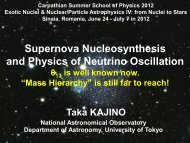
2.7 PropagatorsWe could ask a different question to probe the causal structure of the theory. Preparea particle at spacetime point y. What is the amplitude to find it at point x? We cancalculate this:∫ d 3 p d 3 p ′ 1〈0|φ(x)φ(y) |0〉 = √ 〈0|a(2π) 6 ⃗p a † ⃗p| 0〉 e −ip·x+ip′·y4E⃗p E ′ ⃗p ′∫=d 3 p(2π) 3 12E ⃗pe −ip·(x−y) ≡ D(x − y) (2.90)The function D(x −y) is called the propagator. For spacelike separations, (x −y) 2 < 0,one can show that D(x − y) decays likeD(x − y) ∼ e −m|⃗x−⃗y| (2.91)So it decays exponentially quickly outside the lightcone but, nonetheless, is non-vanishing!The quantum field appears to leak out of the lightcone. Yet we’ve just seen that spacelikemeasurements commute and the theory is causal. How do we reconcile these twofacts? We can rewrite the calculation (2.89) as[φ(x), φ(y)] = D(x − y) − D(y − x) = 0 if (x − y) 2 < 0 (2.92)There are words you can drape around this calculation. When (x − y) 2 < 0, thereis no Lorentz invariant way to order events. If a particle can travel in a spacelikedirection from x → y, it can just as easily travel from y → x. In any measurement, theamplitudes for these two events cancel.With a complex scalar field, it is more interesting. We can look at the equation[ψ(x), ψ † (y)] = 0 outside the lightcone. The interpretation now is that the amplitudefor the particle to propagate from x → y cancels the amplitude for the antiparticleto travel from y → x. In fact, this interpretation is also there for a real scalar fieldbecause the particle is its own antiparticle.2.7.1 The Feynman PropagatorAs we will see shortly, one of the most important quantities in interacting field theoryis the Feynman propagator,∆ F (x − y) = 〈0| Tφ(x)φ(y) |0〉 ={D(x − y) x 0 > y 0D(y − x) y 0 > x 0 (2.93)– 38 –

where T stands for time ordering, placing all operators evaluated at later times to theleft so,{φ(x)φ(y) x 0 > y 0Tφ(x)φ(y) =(2.94)φ(y)φ(x) y 0 > x 0Claim: There is a useful way of writing the Feynman propagator in terms of a 4-momentum integral.∫d 4 p i∆ F (x − y) =e−ip·(x−y) (2.95)(2π) 4 p 2 − m 2Notice that this is the first time in this course that we’ve integrated over 4-momentum.Until now, we integrated only over 3-momentum, with p 0 fixed by the mass-shell conditionto be p 0 = E ⃗p . In the expression (2.95) for ∆ F , we have no such condition onp 0 . However, as it stands this integral is ill-defined because, for each value of ⃗p, thedenominator p 2 −m 2 = (p 0 ) 2 −⃗p 2 −m 2 produces a pole when p 0 = ±E ⃗p = ± √ ⃗p 2 + m 2 .We need a prescription for avoiding these singularities in the p 0 integral. To get theFeynman propagator, we must choose the contour to beIm(p 0)−E p+ E pRe(p 0)Proof:Figure 5: The contour for the Feynman propagator.1p 2 − m = 12 (p 0 ) 2 − E⃗p2=1(p 0 − E ⃗p )(p 0 + E ⃗p )(2.96)so the residue of the pole at p 0 = ±E ⃗p is ±1/2E ⃗p . When x 0 > y 0 , we close the contourin the lower half plane, where p 0 → −i∞, ensuring that the integrand vanishes sincee −ip0 (x 0 −y 0) → 0. The integral over p 0 then picks up the residue at p 0 = +E ⃗p whichis −2πi/2E ⃗p where the minus sign arises because we took a clockwise contour. Hencewhen x 0 > y 0 we have∫∆ F (x − y) =d 3 p(2π) 4 −2πi2E ⃗pi e −iE ⃗p(x 0 −y 0 )+i⃗p·(⃗x−⃗y)– 39 –

∫=d 3 p(2π) 3 12E ⃗pe −ip·(x−y) = D(x − y) (2.97)which is indeed the Feynman propagator for x 0 > y 0 . In contrast, when y 0 > x 0 , weclose the contour in an anti-clockwise direction in the upper half plane to get,∫d 3 p 2πi∆ F (x − y) =(2π) 4 (−2E ⃗p ) i e+iE ⃗p(x 0 −y 0 )+i⃗p·(⃗x−⃗y)∫d 3 p 1= e −iE ⃗p(y 0 −x 0 )−i⃗p·(⃗y−⃗x)(2π) 3 2E ⃗p∫d 3 p 1= e −ip·(y−x) = D(y − x) (2.98)(2π) 3 2E ⃗pwhere to go to from the second line to the third, we have flipped the sign of ⃗p whichis valid since we integrate over d 3 p and all other quantities depend only on ⃗p 2 . Onceagain we reproduce the Feynman propagator.□Instead of specifying the contour, we may instead write Im(p 0 )the Feynman propagator as∫∆ F (x − y) =d 4 p(2π) 4ie −ip·(x−y)p 2 − m 2 + iǫ(2.99)+ iεRe(p 0 )−iεwith ǫ > 0, and infinitesimal. This has the effect of shiftingthe poles slightly off the real axis, so the integral along thereal p 0 axis is equivalent to the contour shown in Figure 5.This way of writing the propagator is, for obvious reasons,called the “iǫ prescription”.Figure 6:2.7.2 Green’s FunctionsThere is another avatar of the propagator: it is a Green’s function for the Klein-Gordonoperator. If we stay away from the singularities, we have∫(∂t 2 − ∇ 2 + m 2 d 4 p i)∆ F (x − y) =(2π) 4 p 2 − m 2 (−p2 + m 2 ) e −ip·(x−y)∫d 4 p= −i e−ip·(x−y)(2π) 4= −i δ (4) (x − y) (2.100)Note that we didn’t make use of the contour anywhere in this derivation. For somepurposes it is also useful to pick other contours which also give rise to Green’s functions.– 40 –

Im(p 0)Im(p 0)−E p+ E pRe(p 0)−E p+E pRe(p 0)Figure 7: The retarded contourFigure 8: The advanced contourFor example, the retarded Green’s function ∆ R (x − y) is defined by the contour shownin Figure 7 which has the property∆ R (x − y) ={D(x − y) − D(y − x) x 0 > y 00 y 0 > x 0 (2.101)The retarded Green’s function is useful in classical field theory if we know the initialvalue of some field configuration and want to figure out what it evolves into in thepresence of a source, meaning that we want to know the solution to the inhomogeneousKlein-Gordon equation,∂ µ ∂ µ φ + m 2 φ = J(x) (2.102)for some fixed background function J(x). Similarly, one can define the advanced Green’sfunction ∆ A (x − y) which vanishes when y 0 < x 0 , which is useful if we know the endpoint of a field configuration and want to figure out where it came from. Given thatnext term’s course is called “Advanced Quantum Field Theory”, there is an obviousname for the current course. But it got shot down in the staff meeting. In the quantumtheory, we will see that the Feynman Green’s function is most relevant.2.8 Non-Relativistic FieldsLet’s return to our classical complex scalar field obeying the Klein-Gordon equation.We’ll decompose the field asThen the KG-equation readsψ(⃗x, t) = e −imt ˜ψ(⃗x, t) (2.103)]∂t 2 ψ − ∇2 ψ + m 2 ψ = e[¨˜ψ −imt − 2im ˙˜ψ − ∇2 ˜ψ = 0 (2.104)with the m 2 term cancelled by the time derivatives. The non-relativistic limit of aparticle is |⃗p| ≪ m. Let’s look at what this does to our field. After a Fourier transform,– 41 –

this is equivalent to saying that |¨˜ψ| ≪ m| ˙˜ψ|. In this limit, we drop the term with twotime derivatives and the KG equation becomes,i ∂ ˜ψ∂t = − 12m ∇2 ˜ψ (2.105)This looks very similar to the Schrödinger equation for a non-relativistic free particle ofmass m. Except it doesn’t have any probability interpretation — it’s simply a classicalfield evolving through an equation that’s first order in time derivatives.We wrote down a Lagrangian in section 1.1.2 which gives rise to field equationswhich are first order in time derivatives. In fact, we can derive this from the relativisticLagrangian for a scalar field by again taking the limit ∂ t ψ ≪ mψ. After losing thetilde, ˜ so ˜ψ → ψ, the non-relativistic Lagrangian becomesL = +iψ ⋆ ˙ψ − 12m ∇ψ⋆ ∇ψ (2.106)where we’ve divided by 1/2m. This Lagrangian has a conserved current arising fromthe internal symmetry ψ → e iα ψ. The current has time and space components()j µ = ψ ⋆ iψ,2m (ψ⋆ ∇ψ − ψ∇ψ ⋆ )(2.107)To move to the Hamiltonian formalism we compute the momentumπ = ∂L∂ ˙ψ = iψ⋆ (2.108)This means that the momentum conjugate to ψ is iψ ⋆ . The momentum does not dependon time derivatives at all! This looks a little disconcerting but it’s fully consistent for atheory which is first order in time derivatives. In order to determine the full trajectoryof the field, we need only specify ψ and ψ ⋆ at time t = 0: no time derivatives on theinitial slice are required.Since the Lagrangian already contains a “p ˙q” term (instead of the more familiar 1 2 p ˙qterm), the time derivatives drop out when we compute the Hamiltonian. We get,H = 12m ∇ψ⋆ ∇ψ (2.109)To quantize we impose (in the Schrödinger picture) the canonical commutation relations[ψ(⃗x), ψ(⃗y)] = [ψ † (⃗x), ψ † (⃗y)] = 0[ψ(⃗x), ψ † (⃗y)] = δ (3) (⃗x − ⃗y) (2.110)– 42 –

We may expand ψ(⃗x) as a Fourier transform∫ψ(⃗x) =where the commutation relations (2.110) required 3 p(2π) 3 a ⃗p ei⃗p·⃗x (2.111)[a ⃗p , a † ⃗q ] = (2π)3 δ (3) (⃗p − ⃗q) (2.112)The vacuum satisfies a ⃗p|0〉 = 0, and the excitations are a † ⃗p 1. . .a † ⃗p n|0〉. The one-particlestates have energyH |⃗p〉 = ⃗p 22m|⃗p〉 (2.113)which is the non-relativistic dispersion relation. We conclude that quantizing the firstorder Lagrangian (2.106) gives rise to non-relativistic particles of mass m. Some comments:• We have a complex field but only a single type of particle. The anti-particle isnot in the spectrum. The existence of anti-particles is a consequence of relativity.• A related fact is that the conserved charge Q = ∫ d 3 x : ψ † ψ : is the particlenumber. This remains conserved even if we include interactions in the Lagrangianof the form∆L = V (ψ ⋆ ψ) (2.114)So in non-relativistic theories, particle number is conserved. It is only with relativity,and the appearance of anti-particles, that particle number can change.• There is no non-relativistic limit of a real scalar field. In the relativistic theory,the particles are their own anti-particles, and there can be no way to construct amulti-particle theory that conserves particle number.2.8.1 Recovering Quantum MechanicsIn quantum mechanics, we talk about the position and momentum operators ⃗ X and⃗P. In quantum field theory, position is relegated to a label. How do we get back toquantum mechanics? We already have the operator for the total momentum of the field∫⃗P =d 3 p(2π) 3 ⃗pa† ⃗p a ⃗p (2.115)– 43 –

which, on one-particle states, gives P ⃗ |⃗p〉 = ⃗p |⃗p〉. It’s also easy to construct the positionoperator. Let’s work in the non-relativistic limit. Then the operator∫ψ † d 3 p(⃗x) =(2π) 3 a† e−i⃗p·⃗x ⃗p(2.116)creates a particle with δ-function localization at ⃗x. We write |⃗x〉 = ψ † (⃗x) |0〉. A naturalposition operator is then∫⃗X = d 3 x ⃗xψ † (⃗x) ψ(⃗x) (2.117)so that ⃗ X |⃗x〉 = ⃗x |⃗x〉.Let’s now construct a state |ϕ〉 by taking superpositions of one-particle states |⃗x〉,∫|ϕ〉 = d 3 x ϕ(⃗x) |⃗x〉 (2.118)The function ϕ(⃗x) is what we would usually call the Schrödinger wavefunction (in theposition representation). Let’s make sure that it indeed satisfies all the right properties.Firstly, it’s clear that acting with the position operator X ⃗ has the right action of ϕ(⃗x),∫X i |ϕ〉 = d 3 x x i ϕ(⃗x) |⃗x〉 (2.119)but what about the momentum operator P? ⃗ We will now show that∫ (P i |ϕ〉 = d 3 x −i ∂ϕ )|⃗x〉 (2.120)∂x iwhich tells us that P i acts as the familiar derivative on wavefunctions |ϕ〉. To see thatthis is the case, we write∫ dP i 3 xd 3 p|ϕ〉 =(2π) 3 pi a † ⃗p a ⃗p ϕ(⃗x) ψ† (⃗x) |0〉∫ d 3 xd 3 p=(2π) 3 pi a † e−i⃗p·⃗x ⃗pϕ(⃗x) |0〉 (2.121)where we’ve used the relationship [a ⃗p, ψ † (⃗x)] = e −i⃗p·⃗x which can be easily checked.Proceeding with our calculation, we have∫ ( dP i 3 xd 3 p|ϕ〉 =(2π) 3 a† ⃗pi ∂ )e−i⃗p·⃗x ϕ(⃗x) |0〉∂x∫ (id 3 xd 3 p= e−i⃗p·⃗x −i ∂ϕ )a †(2π) 3 ∂x i ⃗p |0〉∫ (= d 3 x −i ∂ϕ )|⃗x〉 (2.122)∂x i– 44 –

which confirms (2.120). So we learn that when acting on one-particle states, the operators⃗ X and ⃗ P act as position and momentum operators in quantum mechanics, with[X i , P j ] |ϕ〉 = iδ ij |ϕ〉. But what about dynamics? How does the wavefunction ϕ(⃗x, t)change in time? The Hamiltonian (2.109) can be rewritten asso we find that∫H =d 3 x 1 ∫2m ∇ψ⋆ ∇ψ =d 3 p(2π) 3 ⃗p 22m a† ⃗p a ⃗p (2.123)i ∂ϕ∂t = − 12m ∇2 ϕ (2.124)But this is the same equation obeyed by the original field (2.105)! Except this time, itreally is the Schrödinger equation, complete with the usual probabilistic interpretationfor the wavefunction ϕ. Note in particular that the conserved charge arising from theNoether current (2.107) is Q = ∫ d 3 x |ϕ(⃗x)| 2 which is the total probability.Historically, the fact that the equation for the classical field (2.105) and the oneparticlewavefunction (2.124) coincide caused some confusion. It was thought thatperhaps we are quantizing the wavefunction itself and the resulting name “second quantization”is still sometimes used today to mean quantum field theory. It’s important tostress that, despite the name, we’re not quantizing anything twice! We simply quantizea classical field once. Nonetheless, in practice it’s useful to know that if we treat theone-particle Schrödinger equation as the equation for a quantum field then it will givethe correct generalization to multi-particle states.InteractionsOften in quantum mechanics, we’re interested in particles moving in some fixed backgroundpotential V (⃗x). This can be easily incorporated into field theory by workingwith a Lagrangian with explicit ⃗x dependence,L = iψ ⋆ ˙ψ − 12m ∇ψ⋆ ∇ψ − V (⃗x) ψ ⋆ ψ (2.125)Note that this Lagrangian doesn’t respect translational symmetry and we won’t havethe associated energy-momentum tensor. While such Lagrangians are useful in condensedmatter physics, we rarely (or never) come across them in high-energy physics,where all equations obey translational (and Lorentz) invariance.– 45 –

One can also consider interactions between particles. Obviously these are only importantfor n particle states with n ≥ 2. We therefore expect them to arise from additionsto the Lagrangian of the form∆L = ψ ⋆ (⃗x) ψ ⋆ (⃗x) ψ(⃗x) ψ(⃗x) (2.126)which, in the quantum theory, is an operator which destroys two particles before creatingtwo new ones. Such terms in the Lagrangian will indeed lead to inter-particle forces,both in the non-relativistic and relativistic setting. In the next section we explore thesetypes of interaction in detail for relativistic theories.– 46 –

3. Interacting FieldsThe free field theories that we’ve discussed so far are very special: we can determinetheir spectrum, but nothing interesting then happens. They have particle excitations,but these particles don’t interact with each other.Here we’ll start to examine more complicated theories that include interaction terms.These will take the form of higher order terms in the Lagrangian. We’ll start by askingwhat kind of small perturbations we can add to the theory. For example, consider theLagrangian for a real scalar field,L = 1 2 ∂ µφ ∂ µ φ − 1 2 m2 φ 2 − ∑ n≥3λ nn! φn (3.1)The coefficients λ n are called coupling constants. What restrictions do we have on λ nto ensure that the additional terms are small perturbations? You might think that weneed simply make “λ n ≪ 1”. But this isn’t quite right. To see why this is the case, let’sdo some dimensional analysis. Firstly, note that the action has dimensions of angularmomentum or, equivalently, the same dimensions as . Since we’ve set = 1, usingthe convention described in the introduction, we have [S] = 0. With S = ∫ d 4 x L, and[d 4 x] = −4, the Lagrangian density must therefore have[L] = 4 (3.2)What does this mean for the Lagrangian (3.1)? Since [∂ µ ] = 1, we can read off themass dimensions of all the factors to find,[φ] = 1 , [m] = 1 , [λ n ] = 4 − n (3.3)So now we see why we can’t simply say we need λ n ≪ 1, because this statement onlymakes sense for dimensionless quantities. The various terms, parameterized by λ n , fallinto three different categories• [λ 3 ] = 1: For this term, the dimensionless parameter is λ 3 /E, where E hasdimensions of mass. Typically in quantum field theory, E is the energy scale ofthe process of interest. This means that λ 3 φ 3 /3! is a small perturbation at highenergies E ≫ λ 3 , but a large perturbation at low energies E ≪ λ 3 . Terms thatwe add to the Lagrangian with this behavior are called relevant because they’remost relevant at low energies (which, after all, is where most of the physics we seelies). In a relativistic theory, E > m, so we can always make this perturbationsmall by taking λ 3 ≪ m.– 47 –

• [λ 4 ] = 0: this term is small if λ 4 ≪ 1. Such perturbations are called marginal.• [λ n ] < 0 for n ≥ 5: The dimensionless parameter is (λ n E n−4 ), which is small atlow-energies and large at high energies. Such perturbations are called irrelevant.As you’ll see later, it is typically impossible to avoid high energy processes in quantumfield theory. (We’ve already seen a glimpse of this in computing the vacuum energy).This means that we might expect problems with irrelevant operators. Indeed, these leadto “non-renormalizable” field theories in which one cannot make sense of the infinitiesat arbitrarily high energies. This doesn’t necessarily mean that the theory is useless;just that it is incomplete at some energy scale.Let me note however that the naive assignment of relevant, marginal and irrelevantis not always fixed in stone: quantum corrections can sometimes change the characterof an operator.An Important Aside: Why QFT is SimpleTypically in a quantum field theory, only the relevant and marginal couplings areimportant. This is basically because, as we’ve seen above, the irrelevant couplingsbecome small at low-energies. This is a huge help: of the infinite number of interactionterms that we could write down, only a handful are actually needed (just two in thecase of the real scalar field described above).Let’s look at this a little more. Suppose that we some day discover the true superduper“theory of everything unimportant” that describes the world at very highenergy scales, say the GUT scale, or the Planck scale. Whatever this scale is, let’s callit Λ. It is an energy scale, so [Λ] = 1. Now we want to understand the laws of physicsdown at our puny energy scale E ≪ Λ. Let’s further suppose that down at the energyscale E, the laws of physics are described by a real scalar field. (They’re not of course:they’re described by non-Abelian gauge fields and fermions, but the same argumentapplies in that case so bear with me). This scalar field will have some complicatedinteraction terms (3.1), where the precise form is dictated by all the stuff that’s goingon in the high energy superduper theory. What are these interactions? Well, we couldwrite our dimensionful coupling constants λ n in terms of dimensionless couplings g n ,multiplied by a suitable power of the relevant scale Λ,λ n = g nΛ n−4 (3.4)The exact values of dimensionless couplings g n depend on the details of the high-energysuperduper theory, but typically one expects them to be of order 1: g n ∼ O(1). This– 48 –

means that for experiments at small energies E ≪ Λ, the interaction terms of theform φ n with n > 4 will be suppressed by powers of (E/Λ) n−4 . This is usually asuppression by many orders of magnitude. (e.g for the energies E explored at theLHC, E/M pl ∼ 10 −16 ). It is this simple argument, based on dimensional analysis, thatensures that we need only focus on the first few terms in the interaction: those whichare relevant and marginal. It also means that if we only have access to low-energyexperiments (which we do!), it’s going to be very difficult to figure out the high energytheory (which it is!), because its effects are highly diluted except for the relevant andmarginal interactions. The discussion given above is a poor man’s version of the ideasof effective field theory and Wilson’s renormalization group, about which you can learnmore in the “Statistical Field Theory” course.Examples of Weakly Coupled TheoriesIn this course we’ll study only weakly coupled field theories i.e. ones that can truly beconsidered as small perturbations of the free field theory at all energies. In this section,we’ll look at two types of interactions1) φ 4 theory:L = 1 2 ∂ µφ∂ µ φ − 1 2 m2 φ 2 − λ 4! φ4 (3.5)with λ ≪ 1. We can get a hint for what the effects of this extra term will be. Expandingout φ 4 in terms of a ⃗pand a † ⃗p, we see a sum of interactions that look likea † ⃗p a† ⃗p a† ⃗p a† ⃗pand a † ⃗p a† ⃗p a† ⃗p a ⃗p etc. (3.6)These will create and destroy particles. This suggests that the φ 4 Lagrangian describesa theory in which particle number is not conserved. Indeed, we could check that thenumber operator N now satisfies [H, N] ≠ 0.2) Scalar Yukawa TheoryL = ∂ µ ψ ⋆ ∂ µ ψ + 1 2 ∂ µφ∂ µ φ − M 2 ψ ⋆ ψ − 1 2 m2 φ 2 − gψ ⋆ ψφ (3.7)with g ≪ M, m. This theory couples a complex scalar ψ to a real scalar φ. Whilethe individual particle numbers of ψ and φ are no longer conserved, we do still havea symmetry rotating the phase of ψ, ensuring the existence of the charge Q definedin (2.75) such that [Q, H] = 0. This means that the number of ψ particles minus thenumber of ψ anti-particles is conserved. It is common practice to denote the antiparticleas ¯ψ.– 49 –

The scalar Yukawa theory has a slightly worrying aspect: the potential has a stablelocal minimum at φ = ψ = 0, but is unbounded below for large enough −gφ. Thismeans we shouldn’t try to push this theory too far.A Comment on Strongly Coupled Field TheoriesIn this course we restrict attention to weakly coupled field theories where we can useperturbative techniques. The study of strongly coupled field theories is much moredifficult, and one of the major research areas in theoretical physics. For example, someof the amazing things that can happen include• Charge Fractionalization: Although electrons have electric charge 1, underthe right conditions the elementary excitations in a solid have fractional charge1/N (where N ∈ 2Z + 1). For example, this occurs in the fractional quantumHall effect.• Confinement: The elementary excitations of quantum chromodynamics (QCD)are quarks. But they never appear on their own, only in groups of three (in abaryon) or with an anti-quark (in a meson). They are confined.• Emergent Space: There are field theories in four dimensions which at strongcoupling become quantum gravity theories in ten dimensions! The strong couplingeffects cause the excitations to act as if they’re gravitons moving in higherdimensions. This is quite extraordinary and still poorly understood. It’s calledthe AdS/CFT correspondence.3.1 The Interaction PictureThere’s a useful viewpoint in quantum mechanics to describe situations where we havesmall perturbations to a well-understood Hamiltonian. Let’s return to the familiarground of quantum mechanics with a finite number of degrees of freedom for a moment.In the Schrödinger picture, the states evolve asi d|ψ〉 Sdtwhile the operators O S are independent of time.= H |ψ〉 S(3.8)In contrast, in the Heisenberg picture the states are fixed and the operators changein timeO H (t) = e iHt O S e −iHt|ψ〉 H= e iHt |ψ〉 S(3.9)– 50 –

The interaction picture is a hybrid of the two. We split the Hamiltonian up asH = H 0 + H int (3.10)The time dependence of operators is governed by H 0 , while the time dependence ofstates is governed by H int . Although the split into H 0 and H int is arbitrary, it’s usefulwhen H 0 is soluble (for example, when H 0 is the Hamiltonian for a free field theory).The states and operators in the interaction picture will be denoted by a subscript Iand are given by,|ψ(t)〉 I= e iH 0t |ψ(t)〉 SO I (t) = e iH 0t O S e −iH 0t(3.11)This last equation also applies to H int , which is time dependent. The interactionHamiltonian in the interaction picture is,H I ≡ (H int ) I = e iHot (H int ) S e −iH 0t(3.12)The Schrödinger equation for states in the interaction picture can be derived startingfrom the Schrödinger picturei d|ψ〉 Sdt= H S |ψ〉 S⇒ i d dt⇒i d|ψ〉 Idt(e−iH 0 t |ψ〉 I)= (H0 + H int ) S e −iH 0t |ψ〉 I= e iH 0t (H int ) S e −iH 0t |ψ〉 I(3.13)So we learn thati d|ψ〉 Idt= H I (t) |ψ〉 I(3.14)3.1.1 Dyson’s Formula“Well, Birmingham has much the best theoretical physicist to work with,Peierls; Bristol has much the best experimental physicist, Powell; Cambridgehas some excellent architecture. You can make your choice.”Oppenheimer’s advice to Dyson on which university position to accept.We want to solve (3.14). Let’s write the solution as|ψ(t)〉 I= U(t, t 0 ) |ψ(t 0 )〉 I(3.15)– 51 –

where U(t, t 0 ) is a unitary time evolution operator such that U(t 1 , t 2 )U(t 2 , t 3 ) = U(t 1 , t 3 )and U(t, t) = 1. Then the interaction picture Schrödinger equation (3.14) requires thati dUdt = H I(t) U (3.16)If H I were a function, then we could simply solve this by( ∫ t)U(t, t 0 ) = ? exp −i H I (t ′ ) dt ′ (3.17)t 0But there’s a problem. Our Hamiltonian H I is an operator, and we have orderingissues. Let’s see why this causes trouble. The exponential of an operator is defined interms of the expansion,exp(−i∫ tt 0H I (t ′ ) dt ′ )∫ t(∫ t) 2= 1 − i H I (t ′ ) dt ′ + (−i)2 H I (t ′ ) dt ′ + . . .(3.18)t 02 t 0But when we try to differentiate this with respect to t, we find that the quadratic termgives us− 1 (∫ t)H I (t ′ ) dt ′ H I (t) − 1 (∫ t)2 t 02 H I(t) H I (t ′ ) dt ′ (3.19)t 0Now the second term here looks good, since it will give part of the H I (t)U that weneed on the right-hand side of (3.16). But the first term is no good since the H I (t)sits the wrong side of the integral term, and we can’t commute it through because[H I (t ′ ), H I (t)] ≠ 0 when t ′ ≠ t. So what’s the way around this?Claim: The solution to (3.16) is given by Dyson’s Formula. (Essentially first figuredout by Dirac, although the compact notation is due to Dyson).( ∫ t)U(t, t 0 ) = T exp −i H I (t ′ ) dt ′ (3.20)t 0where T stands for time ordering where operators evaluated at later times are placedto the left{O1 (t 1 ) O 2 (t 2 ) t 1 > t 2T (O 1 (t 1 ) O 2 (t 2 )) =(3.21)O 2 (t 2 ) O 1 (t 1 ) t 2 > t 1Expanding out the expression (3.20), we now have∫ t[∫ t ∫ tU(t, t 0 ) = 1 − i dt ′ H I (t ′ ) + (−i)2 dt ′ dt ′′ H I (t ′′ )H I (t ′ )t 02 t 0 t ′+∫ tt 0dt ′ ∫ t ′t 0dt ′′ H I (t ′ )H I (t ′′ )]+ . . .– 52 –

Actually these last two terms double up since∫ tt 0dt ′ ∫ tt ′ dt ′′ H I (t ′′ )H I (t ′ ) ==∫ tt 0dt ′′ ∫ t ′′∫ tt 0dt ′ ∫ t ′t 0dt ′ H I (t ′′ )H I (t ′ )t 0dt ′′ H I (t ′ )H I (t ′′ ) (3.22)where the range of integration in the first expression is over t ′′ ≥ t ′ , while in the secondexpression it is t ′ ≤ t ′′ which is, of course, the same thing. The final expression is thesame as the second expression by a simple relabelling. This means that we can write∫ t∫ t ∫ t ′U(t, t 0 ) = 1 − i dt ′ H I (t ′ ) + (−i) 2 dt ′ dt ′′ H I (t ′ )H I (t ′′ ) + . . . (3.23)t 0 t 0 t 0Proof: The proof of Dyson’s formula is simpler than explaining what all the notationmeans! Firstly observe that under the T sign, all operators commute (since theirorder is already fixed by the T sign). Thusi ∂ ∫ t)(−i∂t T exp dt ′ H I (t ′ )t 0= T[ ( ∫ tH I (t) exp −i(= H I (t) T exp −i)]dt ′ H I (t ′ )t 0)dt ′ H I (t ′ )t 0∫ t(3.24)since t, being the upper limit of the integral, is the latest time so H I (t) can be pulledout to the left.□Before moving on, I should confess that Dyson’s formula is rather formal. It istypically very hard to compute time ordered exponentials in practice. The power ofthe formula comes from the expansion which is valid when H I is small and is very easilycomputed.3.2 A First Look at ScatteringLet us now apply the interaction picture to field theory, starting with the interactionHamiltonian for our scalar Yukawa theory,∫H int = g d 3 x ψ † ψφ (3.25)Unlike the free theories discussed in Section 2, this interaction doesn’t conserve particlenumber, allowing particles of one type to morph into others. To see why this is, we use– 53 –

the interaction picture and follow the evolution of the state: |ψ(t)〉 = U(t, t 0 ) |ψ(t 0 )〉,where U(t, t 0 ) is given by Dyson’s formula (3.20) which is an expansion in powers ofH int . But H int contains creation and annihilation operators for each type of particle.In particular,• φ ∼ a + a † : This operator can create or destroy φ particles. Let’s call themmesons.• ψ ∼ b + c † : This operator can destroy ψ particles through b, and create antiparticlesthrough c † . Let’s call these particles nucleons. Of course, in realitynucleons are spin 1/2 particles, and don’t arise from the quantization of a scalarfield. But we’ll treat our scalar Yukawa theory as a toy model for nucleonsinteracting with mesons.• ψ † ∼ b † + c: This operator can create nucleons through b † , and destroy antinucleonsthrough c.Importantly, Q = N c − N b remains conserved in the presence of H int . At first order inperturbation theory, we find terms in H int like c † b † a. This kills a meson, producing anucleon-anti-nucleon pair. It will contribute to meson decay φ → ψ ¯ψ.At second order in perturbation theory, we’ll have more complicated terms in (H int ) 2 ,for example (c † b † a)(cba † ). This term will give contributions to scattering processesψ ¯ψ → φ → ψ ¯ψ. The rest of this section is devoted to computing the quantum amplitudesfor these processes to occur.To calculate amplitudes we make an important, and slightly dodgy, assumption:Initial and final states are eigenstates of the free theoryThis means that we take the initial state |i〉 at t → −∞, and the final state |f〉 att → +∞, to be eigenstates of the free Hamiltonian H 0 . At some level, this soundsplausible: at t → −∞, the particles in a scattering process are far separated and don’tfeel the effects of each other. Furthermore, we intuitively expect these states to beeigenstates of the individual number operators N, which commute with H 0 , but notH int . As the particles approach each other, they interact briefly, before departing again,each going on its own merry way. The amplitude to go from |i〉 to |f〉 islim 〈f|U(t +, t − ) |i〉 ≡ 〈f|S |i〉 (3.26)t ± →±∞where the unitary operator S is known as the S-matrix. (S is for scattering). Thereare a number of reasons why the assumption of non-interacting initial and final statesis shaky:– 54 –

• Obviously we can’t cope with bound states. For example, this formalism can’tdescribe the scattering of an electron and proton which collide, bind, and leaveas a Hydrogen atom. It’s possible to circumvent this objection since it turns outthat bound states show up as poles in the S-matrix.• More importantly, a single particle, a long way from its neighbors, is never alonein field theory. This is true even in classical electrodynamics, where the electronsources the electromagnetic field from which it can never escape. In quantumelectrodynamics (QED), a related fact is that there is a cloud of virtual photonssurrounding the electron. This line of thought gets us into the issues of renormalization— more on this next term in the “AQFT” course. Nevertheless, motivatedby this problem, after developing scattering theory using the assumption of noninteractingasymptotic states, we’ll mention a better way.3.2.1 An Example: Meson DecayConsider the relativistically normalized initial and final states,|i〉 = √ 2E ⃗p a † ⃗p |0〉|f〉 = √ 4E ⃗q1 E ⃗q2 b † ⃗q 1c † ⃗q 2|0〉 (3.27)The initial state contains a single meson of momentum p; the final state contains anucleon-anti-nucleon pair of momentum q 1 and q 2 . We may compute the amplitude forthe decay of a meson to a nucleon-anti-nucleon pair. To leading order in g, it is∫〈f|S |i〉 = −ig 〈f| d 4 xψ † (x)ψ(x)φ(x) |i〉 (3.28)Let’s go slowly. We first expand out φ ∼ a + a † using (2.84). (Remember that the φ inthis formula is in the interaction picture, which is the same as the Heisenberg pictureof the free theory). The a piece will turn |i〉 into something proportional to |0〉, whilethe a † piece will turn |i〉 into a two meson state. But the two meson state will havezero overlap with 〈f|, and there’s nothing in the ψ and ψ † operators that lie betweenthem to change this fact. So we have∫〈f|S |i〉 = −ig 〈f|∫= −ig 〈f|∫d 4 xψ † (x)ψ(x)d 3 k(2π) 3 √2E⃗p√2E⃗ka ⃗k a † ⃗p e−ik·x |0〉d 4 xψ † (x)ψ(x)e −ip·x |0〉 (3.29)where, in the second line, we’ve commuted a ⃗k past a † ⃗p , picking up a δ(3) (⃗p − ⃗ k) deltafunctionwhich kills the d 3 k integral. We now similarly expand out ψ ∼ b + c † and– 55 –

ψ † ∼ b † + c. To get non-zero overlap with 〈f|, only the b † and c † contribute, for theycreate the nucleon and anti-nucleon from |0〉. We then have∫ ∫ √d 4 xd 3 k 1 d 3 k 2 E⃗q1 E ⃗q2〈f|S |i〉 = −ig 〈0|(2π) 6 √E⃗k1 cE ⃗q2 b ⃗q1 c † ⃗ k1b † ⃗ k2|0〉 e i(q 1+q 2 −p)·x⃗k2= −ig (2π) 4 δ (4) (q 1 + q 2 − p) (3.30)and so we get our first quantum field theory amplitude.Notice that the δ-function puts constraints on the possible decays. In particular, thedecay only happens at all if m ≥ 2M. To see this, we may always boost ourselvesto a reference frame where the meson is stationary, so p = (m, 0, 0, 0). Then thedelta function imposes momentum conservation, telling us that ⃗q 1 = −⃗q 2 and m =2 √ M 2 + |⃗q| 2 .Later you will learn how to turn this quantum amplitude into something more physical,namely the lifetime of the meson. The reason this is a little tricky is that we mustsquare the amplitude to get the probability for decay, which means we get the squareof a δ-function. We’ll explain how to deal with this in Section 3.6 below, and again innext term’s “Standard Model” course.3.3 Wick’s TheoremFrom Dyson’s formula, we want to compute quantities like 〈f|T {H I (x 1 ) . . .H I (x n )} |i〉,where |i〉 and |f〉 are eigenstates of the free theory. The ordering of the operators is fixedby T, time ordering. However, since the H I ’s contain certain creation and annihilationoperators, our life will be much simpler if we can start to move all annihilation operatorsto the right where they can start killing things in |i〉. Recall that this is the definitionof normal ordering. Wick’s theorem tells us how to go from time ordered products tonormal ordered products.3.3.1 An Example: Recovering the PropagatorLet’s start simple. Consider a real scalar field which we decompose in the Heisenbergpicture aswhereφ(x) = φ + (x) + φ − (x) (3.31)∫φ + (x) =∫φ − (x) =d 3 p 1√ a(2π) 3 ⃗p e −ip·x2E⃗pd 3 p(2π) 3 1√2E⃗pa † ⃗p e+ip·x (3.32)– 56 –

where the ± signs on φ ± make little sense, but apparently you have Pauli and Heisenbergto blame. (They come about because φ + ∼ e −iEt , which is sometimes called the positivefrequency piece, while φ − ∼ e +iEt is the negative frequency piece). Then choosingx 0 > y 0 , we haveT φ(x)φ(y) = φ(x)φ(y)= (φ + (x) + φ − (x))(φ + (y) + φ − (y)) (3.33)= φ + (x)φ + (y) + φ − (x)φ + (y) + φ − (y)φ + (x) + [φ + (x), φ − (y)] + φ − (x)φ − (y)where the last line is normal ordered, and for our troubles we have picked up a factorof D(x − y) = [φ + (x), φ − (y)] which is the propagator we met in (2.90). So for x 0 > y 0we haveT φ(x)φ(y) =: φ(x)φ(y) : + D(x − y) (3.34)Meanwhile, for y 0 > x 0 , we may repeat the calculation to findT φ(x)φ(y) =: φ(x)φ(y) : + D(y − x) (3.35)So putting this together, we have the final expressionT φ(x)φ(y) =: φ(x)φ(y) : + ∆ F (y − x) (3.36)where ∆ F (x − y) is the Feynman propagator defined in (2.93), for which we have theintegral representation∫∆ F (x − y) =d 4 k(2π) 4ie ik·(x−y)k 2 − m 2 + iǫ(3.37)Let me reiterate a comment from Section 2: although T φ(x)φ(y) and : φ(x)φ(y) : areboth operators, the difference between them is a c-number function, ∆ F (x − y).Definition: We define the contraction of a pair of fields in a string of operators. . .φ(x 1 ) . . .φ(x 2 ) . . . to mean replacing those operators with the Feynman propagator,leaving all other operators untouched. We use the notation,to denote contraction. So, for example,. . . { }} {φ(x 1 ) . . .φ(x 2 ) . . . (3.38){ }} {φ(x)φ(y) = ∆ F (x − y) (3.39)– 57 –

A similar discussion holds for complex scalar fields. We haveTψ(x)ψ † (y) =: ψ(x)ψ † (y) : +∆ F (x − y) (3.40)prompting us to define the contraction{ }} {ψ(x)ψ † (y) = ∆ F (x − y) and{ }} { { }} {ψ(x)ψ(y) = ψ † (x)ψ † (y) = 0 (3.41)3.3.2 Wick’s TheoremFor any collection of fields φ 1 = φ(x 1 ), φ 2 = φ(x 2 ), etc, we haveT(φ 1 . . .φ n ) =: φ 1 . . .φ n : + : all possible contractions : (3.42)To see what the last part of this equation means, let’s look at an example. For n = 4,the equation readsT(φ 1 φ 2 φ 3 φ 4 ) = : φ 1 φ 2 φ 3 φ 4 : + {}}{φ 1 φ 2 : φ 3 φ 4 : + φ {}}{1 φ 3 : φ 2 φ 4 : + four similar terms+ {}}{ {}}{φ 1 φ 2 φ 3 φ 4 + φ {}}{ {}}{1 φ 3 φ 2 φ 4 + φ {}}{ {}}{1 φ 4 φ 2 φ 3 (3.43)Proof: The proof of Wick’s theorem proceeds by induction and a little thought. It’strue for n = 2. Suppose it’s true for φ 2 . . . φ n and now add φ 1 . We’ll take x 0 1 > x 0 kfor all k = 2, . . ., n. Then we can pull φ 1 out to the left of the time ordered product,writingT (φ 1 φ 2 . . .φ n ) = (φ + 1 + φ − 1 ) (: φ 2 . . .φ n : + : contractions :) (3.44)The φ − 1 term stays where it is since it is already normal ordered. But in order to writethe right-hand side as a normal ordered product, the φ + 1 term has to make its waypast the crowd of φ − k operators. Each time it moves past φ− k, we pick up a factor of{}}{φ 1 φ k = ∆ F (x 1 − x k ) from the commutator. (Try it!)□3.3.3 An Example: Nucleon ScatteringLet’s look at ψψ → ψψ scattering. We have the initial and final states|i〉 = √ √2E ⃗p1 2E⃗p2 b † ⃗p 1b † ⃗p 2|0〉 ≡ |p 1 , p 2 〉√|f〉 =√2E ⃗p ′12E ⃗p ′2b † ⃗pb † 1′ ⃗p|0〉 ≡ |p ′ 2′ 1 , p 2 ′ 〉 (3.45)We can then look at the expansion of 〈f|S |i〉. In fact, we really want to calculate〈f|S − 1 |i〉 since we’re not interested in situations where no scattering occurs. Atorder g 2 we have the term(−ig) 2 ∫d 4 x 1 d 4 x 2 T ( ψ † (x 1 )ψ(x 1 )φ(x 1 )ψ † (x 2 )ψ(x 2 )φ(x 2 ) ) (3.46)2– 58 –

Now, using Wick’s theorem we see there is a piece in the string of operators which lookslike: ψ † (x 1 )ψ(x 1 )ψ † (x 2 )ψ(x 2 ) :{ }} {φ(x 1 )φ(x 2 ) (3.47)which will contribute to the scattering because the two ψ fields annihilate the ψ particles,while the two ψ † fields create ψ particles. Any other way of ordering the ψ andψ † fields will give zero contribution. This means that we have〈p ′ 1 , p′ 2 | : ψ† (x 1 )ψ(x 1 )ψ † (x 2 )ψ(x 2 ) : |p 1 , p 2 〉= 〈p ′ 1 , p′ 2 |ψ† (x 1 )ψ † (x 2 ) |0〉 〈0|ψ(x 1 )ψ(x 2 ) |p 1 , p 2 〉()= e ip′ 1·x 1+ip ′ 2·x 2+ e ip′ 1·x 2+ip ′ 2·x 1(e−ip 1·x 1 −ip 2·x 2+ e −ip 1·x 2 −ip 2·x 1)= e ix 1·(p ′ 1 −p 1)+ix 2·(p ′ 2 −p 2) + e ix 1·(p ′ 2 −p 1)+ix 2·(p ′ 1 −p 2) + (x 1 ↔ x 2 ) (3.48)where, in going to the third line, we’ve used the fact that for relativistically normalizedstates,〈0|ψ(x) |p〉 = e −ip·x (3.49)Now let’s insert this into (3.46), to get the expression for 〈f|S |i〉 at order g 2 ,(−ig) 2 ∫2d 4 x 1 d 4 x 2[e i... + e i... + (x 1 ↔ x 2 ) ] ∫d 4 k(2π) 4 ie ik·(x 1−x 2 )k 2 − m 2 + iǫ(3.50)where the expression in square brackets is (3.48), while the final integral is the φpropagator which comes from the contraction in (3.47). Now the (x 1 ↔ x 2 ) termsdouble up with the others to cancel the factor of 1/2 out front. Meanwhile, the x 1 andx 2 integrals give delta-functions. We’re left with the expression(−ig) 2 ∫d 4 k(2π) 4 i(2π) 8k 2 − m 2 + iǫ[δ (4) (p ′ 1 − p 1 + k) δ (4) (p ′ 2 − p 2 − k)+ δ (4) (p ′ 2 − p 1 + k) δ (4) (p ′ 1 − p 2 − k) ] (3.51)Finally, we can trivially do the d 4 k integral using the delta-functions to get[]i(−ig) 2 1(p 1 − p 1 ′)2 − m 2 + iǫ + 1(2π) 4 δ (4) (p(p 1 − p 2 ′)2 − m 2 1 + p 2 − p ′ 1 − p ′+ iǫ2)In fact, for this process we may drop the +iǫ terms since the denominator is neverzero. To see this, we can go to the center of mass frame, where ⃗p 1 = −⃗p 2 and, by– 59 –

momentum conservation, |⃗p 1 | = |⃗p 1 ′ |. This ensures that the 4-momentum of the mesonis k = (0, ⃗p − ⃗p ′ ), so k 2 < 0. We therefore have the end result,[]i(−ig) 2 1(p 1 − p 1) ′ 2 − m + 1(2π) 4 δ (4) (p 2 (p 1 − p 2) ′ 2 − m 2 1 + p 2 − p ′ 1 − p ′ 2) (3.52)We will see another, much simpler way to reproduce this result shortly using Feynmandiagrams. This will also shed light on the physical interpretation.This calculation is also relevant for other scattering processes, such as ¯ψ ¯ψ → ¯ψ ¯ψ,ψ ¯ψ → ψ ¯ψ. Each of these comes from the term (3.48) in Wick’s theorem. However, wewill never find a term that contributes to scattering ψψ → ¯ψ ¯ψ, for this would violatethe conservation of Q charge.Another Example: Meson-Nucleon ScatteringIf we want to compute ψφ → ψφ scattering at order g 2 , we would need to pick out theterm: ψ † (x 1 )φ(x 1 )ψ(x 2 )φ(x 2 ) :{ }} {ψ(x 1 )ψ † (x 2 ) (3.53)and a similar term with ψ and ψ † exchanged. Once more, this term also contributes tosimilar scattering processes, including ¯ψφ → ¯ψφ and φφ → ψ ¯ψ.3.4 Feynman Diagrams“Like the silicon chips of more recent years, the Feynman diagram wasbringing computation to the masses.”Julian SchwingerAs the above example demonstrates, to actually compute scattering amplitudes usingWick’s theorem is rather tedious. There’s a much better way. It requires drawing prettypictures. These pictures represent the expansion of 〈f|S |i〉 and we will learn how toassociate numbers (or at least integrals) to them. These pictures are called Feynmandiagrams.The object that we really want to compute is 〈f|S−1 |i〉, since we’re not interested inprocesses where no scattering occurs. The various terms in the perturbative expansioncan be represented pictorially as follows• Draw an external line for each particle in the initial state |i〉 and each particlein the final state |f〉. We’ll choose dotted lines for mesons, and solid lines fornucleons. Assign a directed momentum p to each line. Further, add an arrow to– 60 –

solid lines to denote its charge; we’ll choose an incoming (outgoing) arrow in theinitial state for ψ ( ¯ψ). We choose the reverse convention for the final state, wherean outgoing arrow denotes ψ.ψ• Join the external lines together with trivalent verticesφψ +Each such diagram you can draw is in 1-1 correspondence with the terms in theexpansion of 〈f|S − 1 |i〉.3.4.1 Feynman RulesTo each diagram we associate a number, using the Feynman rules• Add a momentum k to each internal line• To each vertex, write down a factor of(−ig) (2π) 4 δ (4) ( ∑ ik i ) (3.54)where ∑ k i is the sum of all momenta flowing into the vertex.• For each internal dotted line, corresponding to a φ particle with momentum k,we write down a factor of∫d 4 k(2π) 4ik 2 − m 2 + iǫ(3.55)We include the same factor for solid internal ψ lines, with m replaced by thenucleon mass M.– 61 –

3.5 Examples of Scattering AmplitudesLet’s apply the Feynman rules to compute the amplitudes for various processes. Westart with something familiar:Nucleon Scattering RevisitedLet’s look at how this works for the ψψ → ψψ scattering at order g 2 . We can writedown the two simplest diagrams contributing to this process. They are shown in Figure9.p 1/p 1k/p 2p 2+p 1/p2kp / 1p 2Figure 9: The two lowest order Feynman diagrams for nucleon scattering.Applying the Feynman rules to these diagrams, we get[]i(−ig) 2 1(p 1 − p 1 ′)2 − m + 1(2π) 4 δ (4) (p 2 (p 1 − p 2 ′)2 − m 2 1 + p 2 − p ′ 1 − p′ 2 ) (3.56)which agrees with the calculation (3.51) that we performed earlier. There is a nicephysical interpretation of these diagrams. We talk, rather loosely, of the nucleonsexchanging a meson which, in the first diagram, has momentum k = (p 1 −p ′ 1) = (p 2 −p ′ 2).This meson doesn’t satisfy the usual energy dispersion relation, because k 2 ≠ m 2 : themeson is called a virtual particle and is said to be off-shell (or, sometimes, off massshell).Heuristically, it can’t live long enough for its energy to be measured to greataccuracy. In contrast, the momentum on the external, nucleon legs all satisfy p 2 = M 2 ,the mass of the nucleon. They are on-shell. One final note: the addition of the twodiagrams above ensures that the particles satisfy Bose statistics.There are also more complicated diagrams which will contribute to the scatteringprocess at higher orders. For example, we have the two diagrams shown in Figures10 and 11, and similar diagrams with p ′ 1 and p′ 2 exchanged. Using the Feynman rules,each of these diagrams translates into an integral that we will not attempt to calculatehere. And so we go on, with increasingly complicated diagrams, all appearing at higherorder in the coupling constant g.– 62 –

p 1p 1/p 1p 1/p 2p 2/p 2p 2/Figure 10: A contribution at O(g 4 ). Figure 11: A contribution at O(g 6 )AmplitudesOur final result for the nucleon scattering amplitude 〈f|S − 1 |i〉 at order g 2 was[]i(−ig) 2 1(p 1 − p 1 ′)2 − m + 1(2π) 4 δ (4) (p 2 (p 1 − p 2 ′)2 − m 2 1 + p 2 − p 1 ′ − p 2)′The δ-function follows from the conservation of 4-momentum which, in turn, followsfrom spacetime translational invariance. It is common to all S-matrix elements. We willdefine the amplitude A fi by stripping off this momentum-conserving delta-function,〈f|S − 1 |i〉 = i A fi (2π) 4 δ (4) (p F − p I ) (3.57)where p I (p F ) is the sum of the initial (final) 4-momenta, and the factor of i out frontis a convention which is there to match non-relativistic quantum mechanics. We cannow refine our Feynman rules to compute the amplitude iA fi itself:• Draw all possible diagrams with appropriate external legs and impose 4-momentumconservation at each vertex.• Write down a factor of (−ig) at each vertex.• For each internal line, write down the propagator• Integrate over momentum k flowing through each loop ∫ d 4 k/(2π) 4 .This last step deserves a short explanation. The diagrams we’ve computed so far haveno loops. They are tree level diagrams. It’s not hard to convince yourself that intree diagrams, momentum conservation at each vertex is sufficient to determine themomentum flowing through each internal line. For diagrams with loops, such as thoseshown in Figures 10 and 11, this is no longer the case.– 63 –

p 1/p 1/p 2p 2+p 2p 1p /p / 21Figure 12: The two lowest order Feynman diagrams for nucleon to meson scattering.Nucleon to Meson ScatteringLet’s now look at the amplitude for a nucleon-anti-nucleon pair to annihilate into apair of mesons: ψ ¯ψ → φφ. The simplest Feynman diagrams for this process are shownin Figure 12 where the virtual particle in these diagrams is now the nucleon ψ ratherthan the meson φ. This fact is reflected in the denominator of the amplitudes whichare given by[]iA = (−ig) 2 i(p 1 − p 1 ′)2 − M + i(3.58)2 (p 1 − p 2 ′)2 − M 2As in (3.52), we’ve dropped the iǫ from the propagators as the denominator nevervanishes.Nucleon-Anti-Nucleon Scatteringp 1/p 1/p 2p 2+p 1p 1/p 2p 2/Figure 13: The two lowest order Feynman diagrams for nucleon-anti-nucleon scattering.For the scattering of a nucleon and an anti-nucleon, ψ ¯ψ → ψ ¯ψ, the Feynmandiagrams are a little different. At lowest order, they are given by the diagrams ofFigure 13. It is a simple matter to write down the amplitude using the Feynman rules,[]iA = (−ig) 2 i(p 1 − p 1) ′ 2 − m + i(3.59)2 (p 1 + p 2 ) 2 − m 2 + iǫ– 64 –

Notice that the momentum dependence in the secondterm is different from that of nucleon-nucleonscattering (3.56), reflecting the different Feynman diagramthat contributes to the process. In the centerof mass frame, ⃗p 1 = −⃗p 2 , the denominator of the secondterm is 4(M 2 + ⃗p 1) 2 − m 2 . If m < 2M, then thisterm never vanishes and we may drop the iǫ. In contrast,if m > 2M, then the amplitude correspondingto the second diagram diverges at some value of ⃗p.In this case it turns out that we may also neglect theiǫ term, although for a different reason: the mesonis unstable when m > 2M, a result we derived in(3.30). When correctly treated, this instability adds Figure 14:a finite imaginary piece to the denominator whichoverwhelms the iǫ. Nonetheless, the increase in the scattering amplitude which we seein the second diagram when 4(M 2 + ⃗p 2 ) = m 2 is what allows us to discover new particles:they appear as a resonance in the cross section. For example, the Figure 14 showsthe cross-section (roughly the amplitude squared) plotted vertically for e + e − → µ + µ −scattering from the ALEPH experiment in CERN. The horizontal axis shows the centerof mass energy. The curve rises sharply around 91 GeV, the mass of the Z-boson.Meson ScatteringFor φφ → φφ, the simplest diagram we can write/k + p 1pdown has a single loop, and momentum conservation at 1each vertex is no longer sufficient to determine every/k + p 1 − p k1momentum passing through the diagram. We chooseto assign the single undetermined momentum k to thek− p / 2right-hand propagator. All other momenta are then determined.The amplitude corresponding to the diagramshown in the figure isFigure 15:∫ d(−ig) 4 4 k1(2π) 4 (k 2 − M 2 + iǫ)((k + p ′ 1) 2 − M 2 + iǫ)1×((k + p 1 ′ − p 1 ) 2 − M 2 + iǫ)((k − p 2) ′ 2 − M 2 + iǫ)p 2p 1/These integrals can be tricky. For large k, this integral goes as ∫ d 4 k/k 8 , which is atleast convergent as k → ∞. But this won’t always be the case!p / 2– 65 –

3.5.1 Mandelstam VariablesWe see that in many of the amplitudes above — in particular those that include theexchange of just a single particle — the same combinations of momenta are appearingfrequently in the denominators. There are standard names for various sums anddifferences of momenta: they are known as Mandelstam variables. They ares = (p 1 + p 2 ) 2 = (p ′ 1 + p′ 2 )2t = (p 1 − p ′ 1 )2 = (p 2 − p ′ 2 )2 (3.60)u = (p 1 − p ′ 2) 2 = (p 2 − p ′ 1) 2where, as in the examples above, p 1 and p 2 are the momenta of the two initial particles,and p ′ 1 and p ′ 2 are the momenta of the final two particles. We can define these variableswhether the particles involved in the scattering are the same or different. To get a feelfor what these variables mean, let’s assume all four particles are the same. We sit inthe center of mass frame, so that the initial two particles have four-momentap 1 = (E, 0, 0, p) and p 2 = (E, 0, 0, −p) (3.61)The particles then scatter at some angle θ and leave with momentap ′ 1 = (E, 0, p sinθ, p cosθ) and p′ 2 = (E, 0, −p sinθ, −p cosθ) (3.62)Then from the above definitions, we have thats = 4E 2 and t = −2p 2 (1 − cos θ) and u = −2p 2 (1 + cosθ) (3.63)The variable s measures the total center of mass energy of the collision, while thevariables t and u are measures of the momentum exchanged between particles. (Theyare basically equivalent, just with the outgoing particles swapped around). Now theamplitudes that involve exchange of a single particle can be written simply in terms ofthe Mandelstam variables. For example, for nucleon-nucleon scattering, the amplitude(3.56) is schematically A ∼ (t − m 2 ) −1 + (u − m 2 ) −1 . For the nucleon-anti-nucleonscattering, the amplitude (3.59) is A ∼ (t − m 2 ) −1 + (s − m 2 ) −1 . We say that thefirst case involves “t-channel” and “u-channel” diagrams. Meanwhile the nucleon-antinucleonscattering is said to involve “t-channel” and “s-channel” diagrams. (The firstdiagram indeed includes a vertex that looks like the letter “T”).Note that there is a relationship between the Mandelstam variables. When all themasses are the same we have s+t+u = 4M 2 . When the masses of all 4 particles differ,this becomes s + t + u = ∑ i M2 i . – 66 –

3.5.2 The Yukawa PotentialSo far we’ve computed the quantum amplitudes for various scattering processes. Butthese quantities are a little abstract. In Section 3.6 below (and again in next term’s“Standard Model” course) we’ll see how to turn amplitudes into measurable quantitiessuch as cross-sections, or the lifetimes of unstable particles. Here we’ll instead showhow to translate the amplitude (3.52) for nucleon scattering into something familiarfrom Newtonian mechanics: a potential, or force, between the particles.Let’s start by asking a simple question in classical field theory that will turn out tobe relevant. Suppose that we have a fixed δ-function source for a real scalar field φ,that persists for all time. What is the profile of φ(⃗x)? To answer this, we must solvethe static Klein-Gordon equation,−∇ 2 φ + m 2 φ = δ (3) (⃗x) (3.64)We can solve this using the Fourier transform,∫ d 3 kφ(⃗x) =(2π) 3 ei⃗ k·⃗x ˜φ( ⃗ k) (3.65)Plugging this into (3.64) tells us that ( ⃗ k 2 + m 2 )˜φ( ⃗ k) = 1, giving us the solution∫φ(⃗x) =d 3 k(2π) 3e i⃗ k·⃗x⃗ k 2+ m 2 (3.66)Let’s now do this integral. Changing to polar coordinates, and writing ⃗ k · ⃗x = kr cosθ,we haveφ(⃗x) = 1 ∫ ∞dk(2π) 2=1(2π) 2 r0∫ +∞−∞= 12πr Re [∫ +∞−∞k 2 2 sin krk 2 + m 2 krdkk sin krk 2 + m 2]ke ikrk 2 + m 2dk2πi(3.67)We compute this last integral by closing the contour in the upper half plane k → +i∞,picking up the pole at k = +im. This givesφ(⃗x) = 14πr e−mr (3.68)The field dies off exponentially quickly at distances 1/m, the Compton wavelength ofthe meson.– 67 –

Now we understand the profile of the φ field, what does this have to do with the forcebetween ψ particles? We do very similar calculations to that above in electrostaticswhere a charged particle acts as a δ-function source for the gauge potential: −∇ 2 A 0 =δ (3) (⃗x), which is solved by A 0 = 1/4πr. The profile for A 0 then acts as the potentialenergy for another charged (test) particle moving in this background. Can we give thesame interpretation to our scalar field? In other words, is there a classical limit of thescalar Yukawa theory where the ψ particles act as δ-function sources for φ, creatingthe profile (3.68)? And, if so, is this profile then felt as a static potential? The answeris essentially yes, at least in the limit M ≫ m. But the correct way to describe thepotential felt by the ψ particles is not to talk about classical fields at all, but insteadwork directly with the quantum amplitudes.Our strategy is to compare the nucleon scattering amplitude (3.52) to the correspondingamplitude in non-relativistic quantum mechanics for two particles interactingthrough a potential. To make this comparison, we should first take the non-relativisticlimit of (3.52). Let’s work in the center of mass frame, with ⃗p ≡ ⃗p 1 = −⃗p 2 and⃗p ′ ≡ ⃗p 1 ′ = −⃗p 2 ′ . The non-relativistic limit means |⃗p| ≪ M which, by momentumconservation, ensures that |⃗p ′ | ≪ M. In fact one can check that, for this particularexample, this limit doesn’t change the scattering amplitude (3.52): it’s given by[]iA = +ig 2 1(⃗p − ⃗p ′ ) 2 + m + 1(3.69)2 (⃗p + ⃗p ′ ) 2 + m 2How do we compare this to scattering in quantum mechanics? Consider two particles,separated by a distance ⃗r, interacting through a potential U(⃗r). In non-relativisticquantum mechanics, the amplitude for the particles to scatter from momentum states±⃗p into momentum states ±⃗p ′ can be computed in perturbation theory, using thetechniques described in Section 3.1. To leading order, known in this context as theBorn approximation, the amplitude is given by∫〈⃗p ′ |U(⃗r) |⃗p 〉 = −i d 3 r U(⃗r)e −i(⃗p−⃗p′ )·⃗r(3.70)There’s a relative factor of (2M) 2 that arises in comparing the quantum field theoryamplitude A to 〈⃗p ′ |U(⃗r) |⃗p〉, that can be traced to the relativistic normalization of thestates |p 1 , p 2 〉. (It is also necessary to get the dimensions of the potential to work outcorrectly). Including this factor, and equating the expressions for the two amplitudes,we get∫d 3 r U(⃗r) e −i(⃗p−⃗p′ )·⃗r −λ 2=(3.71)(⃗p − ⃗p ′ ) 2 + m 2– 68 –

where we’ve introduced the dimensionless parameter λ = g/2M. We can trivially invertthis to find,U(⃗r) = −λ 2 ∫d 3 p(2π) 3e i⃗p·⃗r⃗p 2 + m 2 (3.72)But this is exactly the integral (3.66) we just did in the classical theory. We haveU(⃗r) = −λ24πr e−mr (3.73)This is the Yukawa potential. The force has a range 1/m, the Compton wavelength ofthe exchanged particle. The minus sign tells us that the potential is attractive.Notice that quantum field theory has given us an entirely new perspective on thenature of forces between particles. Rather than being a fundamental concept, the forcearises from the virtual exchange of other particles, in this case the meson. In Section 6of these lectures, we will see how the Coulomb force arises from quantum field theorydue to the exchange of virtual photons.We could repeat the calculation for nucleon-anti-nucleon scattering. The amplitudefrom field theory is given in (3.59). The first term in this expression gives the sameresult as for nucleon-nucleon scattering with the same sign. The second term vanishes inthe non-relativisitic limit (it is an example of an interaction that doesn’t have a simpleNewtonian interpretation). There is no longer a factor of 1/2 in (3.70), because theincoming/outgoing particles are not identical, so we learn that the potential betweena nucleon and anti-nucleon is again given by (3.73). This reveals a key feature offorces arising due to the exchange of scalars: they are universally attractive. Noticethat this is different from forces due to the exchange of a spin 1 particle — such aselectromagnetism — where the sign flips when we change the charge. However, forforces due to the exchange of a spin 2 particle — i.e. gravity — the force is againuniversally attractive.3.5.3 φ 4 TheoryLet’s briefly look at the Feynman rules and scattering amplitudes for the interactionHamiltonianH int = λ 4! φ4 (3.74)The theory now has a single interaction vertex, which comes with a factor of (−iλ),while the other Feynman rules remain the same. Note that we assign (−iλ) to the– 69 –

vertex rather than (−iλ/4!). To see why this is, we can look at φφ → φφ scattering,which has its lowest contribution at order λ, with the term−iλ4!〈p ′ 1 , p ′ 2 | : φ(x)φ(x)φ(x)φ(x) : |p 1, p 2 〉 (3.75)Any one of the fields can do the job of annihilation or creation. This gives 4! differentcontractions, which cancels the 1/4! sitting out front.Feynman diagrams in the φ 4 theory sometimes come with extracombinatoric factors (typically 2 or 4) which are known as symmetryfactors that one must take into account. For more details, see the bookby Peskin and Schroeder.−iλUsing the Feynman rules, the scattering amplitude for φφ → φφ is Figure 16:simply iA = −iλ. Note that it doesn’t depend on the angle at whichthe outgoing particles emerge: in φ 4 theory the leading order two-particle scatteringoccurs with equal probability in all directions. Translating this into a potential betweentwo mesons, we haveU(⃗r) =λ ∫(2m) 2d 3 p(2π) 3 e+i⃗p·⃗r =λ(2m) 2δ(3) (⃗r) (3.76)So scattering in φ 4 theory is due to a δ-function potential. The particles don’t knowwhat hit them until it’s over.3.5.4 Connected Diagrams and Amputated DiagramsWe’ve seen how one can compute scattering amplitudes by writing down all Feynmandiagrams and assigning integrals to them using the Feynman rules. In fact, there area couple of caveats about what Feynman diagrams you should write down. Both ofthese caveats are related to the assumption we made earlier that “initial and final statesare eigenstates of the free theory” which, as we mentioned at the time, is not strictlyaccurate. The two caveats which go some way towards ameliorating the problem arethe following• We consider only connected Feynman diagrams, where every part of the diagramis connected to at least one external line. As we shall see shortly, this will berelated to the fact that the vacuum |0〉 of the free theory is not the true vacuum|Ω〉 of the interacting theory. An example of a diagram that is not connected isshown in Figure 17.– 70 –

• We do not consider diagrams with loops on external lines, for example the diagramshown in the Figure 18. We will not explain how to take these into account in thiscourse, but you will discuss them next term. They are related to the fact that theone-particle states of the free theory are not the same as the one-particle states ofthe interacting theory. In particular, correctly dealing with these diagrams willaccount for the fact that particles in interacting quantum field theories are neveralone, but surrounded by a cloud of virtual particles. We will refer to diagramsin which all loops on external legs have been cut-off as “amputated”.Figure 17: A disconnected diagram.Figure 18: An un-amputated diagram3.6 What We Measure: Cross Sections and Decay RatesSo far we’ve learnt to compute the quantum amplitudes for particles decaying or scattering.As usual in quantum theory, the probabilities for things to happen are the(modulus) square of the quantum amplitudes. In this section we will compute theseprobabilities, known as decay rates and cross sections. One small subtlety here is thatthe S-matrix elements 〈f|S − 1 |i〉 all come with a factor of (2π) 4 δ (4) (p F − p I ), so weend up with the square of a delta-function. As we will now see, this comes from thefact that we’re working in an infinite space.3.6.1 Fermi’s Golden RuleLet’s start with something familiar and recall how to derive Fermi’s golden rule fromDyson’s formula. For two energy eigenstates |m〉 and |n〉, with E m ≠ E n , we have toleading order in the interaction,〈m|U(t) |n〉 = −i 〈m|∫ t= −i 〈m|H int |n〉0dt H I (t) |n〉∫ t= − 〈m| H int |n〉 eiωt − 1ω0dt ′ e iωt′(3.77)– 71 –

where ω = E m −E n . This gives us the probability for the transition from |n〉 to |m〉 intime t, as( ) 1 − cosωtP n→m (t) = | 〈m| U(t) |n〉 | 2 = 2| 〈m| H int |n〉 | 2 (3.78)ω 2The function in brackets is plotted in Figure 19 for fixed t.We see that in time t, most transitions happen in a regionbetween energy eigenstates separated by ∆E = 2π/t. Ast → ∞, the function in the figure starts to approach a deltafunction.To find the normalization, we can calculate⇒∫ +∞( ) 1 − cos ωtdω = πt−∞ ω( )21 − cosωt→ πtδ(ω) asω 2t → ∞Figure 19:Consider now a transition to a cluster of states with densityρ(E). In the limit t → ∞, we get the transition probability∫( ) 1 − cosωtP n→m = dE m ρ(E m ) 2| 〈m|H int |n〉 | 2 ω 2→ 2π | 〈m| H int |n〉 | 2 ρ(E n )t (3.79)which gives a constant probability for the transition per unit time for states aroundthe same energy E n ∼ E m = E.This is Fermi’s Golden Rule.˙ P n→m = 2π| 〈m|H int |n〉 | 2 ρ(E) (3.80)In the above derivation, we were fairly careful with taking the limit as t → ∞.Suppose we were a little sloppier, and first chose to compute the amplitude for thestate |n〉 at t → −∞ to transition to the state |m〉 at t → +∞. Then we get−i 〈m|∫ t=+∞t=−∞H I (t) |n〉 = −i 〈m|H int |n〉 2πδ(ω) (3.81)Now when squaring the amplitude to get the probability, we run into the problem ofthe square of the delta-function: P n→m = | 〈m| H int |n〉 | 2 (2π) 2 δ(ω) 2 . Tracking throughthe previous computations, we realize that the extra infinity is coming because P m→n– 72 –

is the probability for the transition to happen in infinite time t → ∞. We can writethe delta-functions as(2π) 2 δ(ω) 2 = (2π)δ(ω) T (3.82)where T is shorthand for t → ∞ (we used a very similar trick when looking at thevacuum energy in (2.25)). We now divide out by this power of T to get the transitionprobability per unit time,˙ P n→m = 2π| 〈m| H int |n〉 | 2 δ(ω) (3.83)which, after integrating over the density of final states, gives us back Fermi’s Goldenrule. The reason that we’ve stressed this point is because, in our field theory calculations,we’ve computed the amplitudes in the same way as (3.81), and the square of theδ (4) -functions will just be re-interpreted as spacetime volume factors.3.6.2 Decay RatesLet’s now look at the probability for a single particle |i〉 of momentum p I (I=initial)to decay into some number of particles |f〉 with momentum p i and total momentump F = ∑ i p i. This is given byP =| 〈f|S |i〉 |2〈f|f〉 〈i| i〉(3.84)Our states obey the relativistic normalization formula (2.65),〈i|i〉 = (2π) 3 2E ⃗pI δ (3) (0) = 2E ⃗pI V (3.85)where we have replaced δ (3) (0) by the volume of 3-space. Similarly,〈f|f〉 =∏2E ⃗pi V (3.86)final statesIf we place our initial particle at rest, so ⃗p I = 0 and E ⃗pI = m, we get the probabilityfor decayP = |A fi| 22mV (2π)4 δ (4) (p I − p F ) V T∏final states12E ⃗pi V(3.87)where, as in the second derivation of Fermi’s Golden Rule, we’ve exchanged one of thedelta-functions for the volume of spacetime: (2π) 4 δ (4) (0) = V T. The amplitudes A fiare, of course, exactly what we’ve been computing. (For example, in (3.30), we saw– 73 –

that A = −g for a single meson decaying into two nucleons). We can now divide outby T to get the transition function per unit time. But we still have to worry aboutsumming over all final states. There are two steps: the first is to integrate over allpossible momenta of the final particles: V ∫ d 3 p i /(2π) 3 . The factors of spatial volumeV in this measure cancel those in (3.87), while the factors of 1/2E ⃗pi in (3.87) conspireto produce the Lorentz invariant measure for 3-momentum integrals. The result is anexpression for the density of final states given by the Lorentz invariant measuredΠ = (2π) 4 δ (4) (p F − p I )∏final statesd 3 p i(2π) 3 12E ⃗pi(3.88)The second step is to sum over all final states with different numbers (and possiblytypes) of particles. This gives us our final expression for the decay probability per unittime, Γ = P. ˙Γ = 1 ∑∫|A fi | 2 dΠ (3.89)2mfinal statesΓ is called the width of the particle. It is equal to the reciprocal of the half-life τ = 1/Γ.3.6.3 Cross SectionsCollide two beams of particles. Sometimes the particles will hit and bounce off eachother; sometimes they will pass right through. The fraction of the time that they collideis called the cross section and is denoted by σ. If the incoming flux F is defined tobe the number of incoming particles per area per unit time, then the total number ofscattering events N per unit time is given by,N = Fσ (3.90)We would like to calculate σ from quantum field theory. In fact, we can calculate a moresensitive quantity dσ known as the differential cross section which is the probabilityfor a given scattering process to occur in the solid angle (θ, φ). More preciselydσ =Differential ProbabilityUnit Time × Unit Flux = 14E 1 E 2 V1F |A fi| 2 dΠ (3.91)where we’ve used the expression for probability per unit time that we computed in theprevious subsection. E 1 and E 2 are the energies of the incoming particles. We nowneed an expression for the unit flux. For simplicity, let’s sit in the center of mass frameof the collision. We’ve been considering just a single particle per spatial volume V ,– 74 –

meaning that the flux is given in terms of the 3-velocities ⃗v i as F = |⃗v 1 − ⃗v 2 |/V . Thisthen gives,dσ = 14E 1 E 21|⃗v 1 − ⃗v 2 | |A fi| 2 dΠ (3.92)If you want to write this in terms of momentum, then recall from your course on specialrelativity that the 3-velocities ⃗v i are related to the momenta by ⃗v = ⃗p/m √ 1 − v 2 =⃗p/p 0 .Equation (3.92) is our final expression relating the S-matrix to the differential crosssection. You may now take your favorite scattering amplitude, and compute the probabilityfor particles to fly out at your favorite angles. This will involve doing the integralover the phase space of final states, with measure dΠ. Notice that different scatteringamplitudes have different momentum dependence and will result in different angulardependence in scattering amplitudes. For example, in φ 4 theory the amplitude for treelevel scattering was simply A = −λ. This results in isotropic scattering. In contrast,for nucleon-nucleon scattering we have schematically A ∼ (t − m 2 ) −1 + (u − m 2 ) −1 .This gives rise to angular dependence in the differential cross-section, which followsfrom the fact that, for example, t = −2|⃗p| 2 (1 −cos θ), where θ is the angle between theincoming and outgoing particles.3.7 Green’s FunctionsSo far we’ve learnt to compute scattering amplitudes. These are nice and physical (well– they’re directly related to cross-sections and decay rates which are physical) but thereare many questions we want to ask in quantum field theory that aren’t directly relatedto scattering experiments. For example, we might want to compute the viscosity ofthe quark gluon plasma, or the optical conductivity in a tentative model of strangemetals, or figure out the non-Gaussianity of density perturbations arising in the CMBfrom novel models of inflation. All of these questions are answered in the framework ofquantum field theory by computing elementary objects known as correlation functions.In this section we will briefly define correlation functions, explain how to compute themusing Feynman diagrams, and then relate them back to scattering amplitudes. We’llleave the relationship to other physical phenomena to other courses.We’ll denote the true vacuum of the interacting theory as |Ω〉. We’ll normalize Hsuch thatH |Ω〉 = 0 (3.93)– 75 –

and 〈Ω| Ω〉 = 1. Note that this is different from the state we’ve called |0〉 which is thevacuum of the free theory and satisfies H 0 |0〉 = 0. DefineG (n) (x 1 , . . .,x n ) = 〈Ω| T φ H (x 1 ) . . .φ H (x n ) |Ω〉 (3.94)where φ H is φ in the Heisenberg picture of the full theory, rather than the interactionpicture that we’ve been dealing with so far. The G (n) are called correlation functions,or Green’s functions. There are a number of different ways of looking at these objectswhich tie together nicely. Let’s start by asking how to compute G (n) using Feynmandiagrams. We prove the following resultClaim: We use the notation φ 1 = φ(x 1 ), and write φ 1H to denote the field in theHeisenberg picture, and φ 1I to denote the field in the interaction picture. ThenG (n) (x 1 , . . .,x n ) = 〈Ω|T φ 1H . . . φ nH |Ω〉 = 〈0|Tφ 1I . . .φ nI S |0〉〈0|S |0〉(3.95)where the operators on the right-hand side are evaluated on |0〉, the vacuum of the freetheory.Proof: Take t 1 > t 2 > . . . > t n . Then we can drop the T and write the numeratorof the right-hand side as〈0|U I (+∞, t 1 )φ 1I U(t 1 , t 2 ) φ 2I . . . φ nI U I (t n , −∞) |0〉= 〈0|U I (+∞, t 1 )φ 1H . . .φ nH U I (t n , −∞) |0〉where we’ve used all the intermediate factors of U I (t k , t k+1 ) = T exp(−i ∫ t k+1t kH I ) toconvert φ I into φ H . Now let’s deal with the two remaining U(t, ±∞) at either end ofthe string of operators. Consider an arbitrary state |Ψ〉〈Ψ|U I (t, −∞) |0〉 = 〈Ψ|U(t, −∞) |0〉 (3.96)where U(t, −∞) is the Schrödinger evolution operator, and the equality above followsbecause H 0 |0〉 = 0. Now insert a complete set of states, which we take to be energyeigenstates of H = H 0 + H int ,[]〈Ψ|U(t, −∞) |0〉 = 〈Ψ|U(t, −∞) |Ω〉 〈Ω| + ∑ |n〉 〈n| |0〉n≠0∑= 〈Ψ| Ω〉 〈Ω| 0〉 + lim e iEn(t′ −t) 〈Ψ|n〉 〈n| 0〉 (3.97)t ′ →−∞n≠0– 76 –

But the last term vanishes. This follows from the Riemann-Lebesgue lemma which saysthat for any well-behaved function∫ blimµ→∞adxf(x)e iµx = 0 (3.98)Why is this relevant? The point is that the ∑ n in (3.97) is really an integral ∫ dn,because all states are part of a continuum due to the momentum. (There is a caveathere: we want the vacuum |Ω〉 to be special, so that it sits on its own, away from thecontinuum of the integral. This means that we must be working in a theory with amass gap – i.e. with no massless particles). So the Riemann-Lebesgue lemma gives uslim 〈Ψ|U(t,t ′ →−∞ t′ ) |0〉 = 〈Ψ| Ω〉 〈Ω| 0〉 (3.99)(Notice that to derive this result, Peskin and Schroeder instead send t → −∞ in aslightly imaginary direction, which also does the job). We now apply the formula(3.99), to the top and bottom of the right-hand side of (3.95) to find〈0| Ω〉 〈Ω| Tφ 1H . . .φ nH |Ω〉 〈Ω| 0〉〈0| Ω〉 〈Ω| Ω〉 〈Ω| 0〉(3.100)which, using the normalization 〈Ω| Ω〉 = 1, gives us the left-hand side, completing theproof. □.3.7.1 Connected Diagrams and Vacuum BubblesWe’re getting closer to our goal of computing the Green’s functions G (n) since wecan compute both 〈0|Tφ I (x 1 ) . . .φ I (x n ) S |0〉 and 〈0| S |0〉 using the same methodswe developed for S-matrix elements; namely Dyson’s formula and Wick’s theorem or,alternatively, Feynman diagrams. But what about dividing one by the other? What’sthat all about? In fact, it has a simple interpretation. For the following discussion,we will work in φ 4 theory. Since there is no ambiguity in the different types of linein Feynman diagrams, we will represent the φ particles as solid lines, rather than thedashed lines that we used previously. Then we have the diagramatic expansion for〈0|S |0〉.〈0|S |0〉 = 1 + +( + + ) + . . . (3.101)These diagrams are called vacuum bubbles. The combinatoric factors (as well as thesymmetry factors) associated with each diagram are such that the whole series sums– 77 –

to an exponential,〈0|S |0〉 = exp( + + + ...)(3.102)So the amplitude for the vacuum of the free theory to evolve into itself is 〈0|S |0〉 =exp(all distinct vacuum bubbles). A similar combinatoric simplification occurs for genericcorrelation functions. Remarkably, the vacuum diagrams all add up to give the sameexponential. With a little thought one can show that(∑ )〈0|Tφ 1 . . .φ n |0〉 = connected diagrams 〈0|S |0〉 (3.103)where “connected” means that every part of the diagram is connected to at least oneof the external legs. The upshot of all this is that dividing by 〈0| S |0〉 has a very niceinterpretation in terms of Feynman diagrams: we need only consider the connectedFeynman diagrams, and don’t have to worry about the vacuum bubbles. Combiningthis with (3.95), we learn that the Green’s functions G (n) (x 1 . . .,x n ) can be calculatedby summing over all connected Feynman diagrams,〈Ω| T φ H (x 1 ) . . .φ H (x n ) |Ω〉 = ∑ Connected Feynman Graphs (3.104)An Example: The Four-Point Correlator: 〈Ω|Tφ H (x 1 ) . . .φ H (x 4 ) |Ω〉As a simple example, let’s look at the four-point correlation function in φ 4 theory. Thesum of connected Feynman diagrams is given by,xx 1 x 2x 1 x 1 x 222 Similarx 3 x 4 x 3 x 4 x 3 x 4+ + + + 5 Similar + ...All of these are connected diagrams, even though they don’t look x 1 x 2that connected! The point is that a connected diagram is definedby the requirement that every line is joined to an external leg. Anexample of a diagram that is not connected is shown in the figure.As we have seen, such diagrams are taken care of in shifting thevacuum from |0〉 to |Ω〉.x 3 x 4Figure 20:Feynman RulesThe Feynman diagrams that we need to calculate for the Green’s functions depend onx 1 , . . .,x n . This is rather different than the Feynman diagrams that we calculated for– 78 –

the S-matrix elements, where we were working primarily with momentum eigenstates,and ended up integrating over all of space. However, it’s rather simple to adapt theFeynman rules that we had earlier in momentum space to compute G (n) (x 1 . . .,x n ).For φ 4 theory, we have• Draw n external points x 1 , . . ., x n , connected by the usual propagators and vertices.Assign a spacetime position y to the end of each line.• For each line x∆ F (x − y).y from x to y write down a factor of the Feynman propagator• For each vertex y at position y, write down a factor of −iλ ∫ d 4 y.3.7.2 From Green’s Functions to S-MatricesHaving described how to compute correlation functions using Feynman diagrams, let’snow relate them back to the S-matrix elements that we already calculated. The firststep is to perform the Fourier transform,∫ [ n]∏˜G (n) (p 1 , . . .,p n ) = d 4 x i e −ip i·x iG (n) (x 1 , . . .,x n ) (3.105)i=1These are very closely related to the S-matrix elements that we’ve computed above. Thedifference is that the Feynman rules for G (n) (x 1 , . . .,x n ), effectively include propagators∆ F for the external legs, as well as the internal legs. A related fact is that the 4-momenta assigned to the external legs is arbitrary: they are not on-shell. Both of theseproblems are easily remedied to allow us to return to the S-matrix elements: we needto simply cancel off the propagators on the external legs, and place their momentumback on shell. We have〈p ′ 1 , . . .,p′ n ′|S − 1 |p ∏n ′n∏1 . . .,p n 〉 = (−i) n+n′ (p i ′ 2 − m 2 ) (p 2 j − m2 ) (3.106)i=1j=1× ˜G (n+n′) (−p ′ 1 , . . .,−p′ n ′, p 1, . . ., p n )Each of the factors (p 2 −m 2 ) vanishes once the momenta are placed on-shell. This meansthat we only get a non-zero answer for diagrams contributing to G (n) (x 1 , . . .,x n ) whichhave propagators for each external leg. You might think they all do, but it’s not true!Only diagrams that are fully connected, meaning each external point is connected toeach other external point, have this property. For example, of the diagrams that wewrote down which contribute to the four-point function 〈Ω| Tφ H (x 1 ) . . .φ H (x 4 ) |Ω〉, onlywill survive the multiplication by on-shell propagators in (3.106) to contribute tothe S-matrix for meson scattering in φ 4 theory.– 79 –

So what’s the point of all of this? We’ve understood that ignoring the connecteddiagrams is related to shifting to the true vacuum |Ω〉. But other than that, introducingthe Green’s functions seems like a lot of bother for little reward. The important pointis that this provides a framework in which to deal with the true particle states inthe interacting theory through renormalization. Indeed, the formula (3.106), suitablyinterpreted, remains true even in the interacting theory, taking into account the swarmof virtual particles surrounding asymptotic states. This is the correct way to considerscattering. In this context, (3.106) is known as the LSZ reduction formula. You willderive it properly next term.– 80 –

4. The Dirac Equation“A great deal more was hidden in the Dirac equation than the author hadexpected when he wrote it down in 1928. Dirac himself remarked in one ofhis talks that his equation was more intelligent than its author. It shouldbe added, however, that it was Dirac who found most of the additionalinsights.”Weisskopf on DiracSo far we’ve only discussed scalar fields such that under a Lorentz transformationx µ → (x ′ ) µ = Λ µ νx ν , the field transforms asφ(x) → φ ′ (x) = φ(Λ −1 x) (4.1)We have seen that quantization of such fields gives rise to spin 0 particles. But mostparticles in Nature have an intrinsic angular momentum, or spin. These arise naturallyin field theory by considering fields which themselves transform non-trivially under theLorentz group. In this section we will describe the Dirac equation, whose quantizationgives rise to fermionic spin 1/2 particles. To motivate the Dirac equation, we will startby studying the appropriate representation of the Lorentz group.A familiar example of a field which transforms non-trivially under the Lorentz groupis the vector field A µ (x) of electromagnetism,A µ (x) → Λ µ ν Aν (Λ −1 x) (4.2)We’ll deal with this in Section 6. (It comes with its own problems!). In general, a fieldcan transform asφ a (x) → D[Λ] a b φ b (Λ −1 x) (4.3)where the matrices D[Λ] form a representation of the Lorentz group, meaning thatD[Λ 1 ]D[Λ 2 ] = D[Λ 1 Λ 2 ] (4.4)and D[Λ −1 ] = D[Λ] −1 and D[1] = 1. How do we find the different representations?Typically, we look at infinitesimal transformations of the Lorentz group and study theresulting Lie algebra. If we write,Λ µ ν = δµ ν + ωµ ν (4.5)for infinitesimal ω, then the condition for a Lorentz transformation Λ µ σ Λν ρ ησρ = η µνbecomes the requirement that ω is anti-symmetric:ω µν + ω νµ = 0 (4.6)– 81 –

Note that an antisymmetric 4 × 4 matrix has 4 × 3/2 = 6 independent components,which agrees with the 6 transformations of the Lorentz group: 3 rotations and 3 boosts.It’s going to be useful to introduce a basis of these six 4 × 4 anti-symmetric matrices.We could call them (M A ) µν , with A = 1, . . .,6. But in fact it’s better for us (althoughinitially a little confusing) to replace the single index A with a pair of antisymmetricindices [ρσ], where ρ, σ = 0, . . .,3, so we call our matrices (M ρσ ) µ ν. The antisymmetryon the ρ and σ indices means that, for example, M 01 = −M 10 , etc, so that ρ and σagain label six different matrices. Of course, the matrices are also antisymmetric onthe µν indices because they are, after all, antisymmetric matrices. With this notationin place, we can write a basis of six 4 × 4 antisymmetric matrices as(M ρσ ) µν = η ρµ η σν − η σµ η ρν (4.7)where the indices µ and ν are those of the 4 × 4 matrix, while ρ and σ denote whichbasis element we’re dealing with. If we use these matrices for anything practical (forexample, if we want to multiply them together, or act on some field) we will typicallyneed to lower one index, so we have(M ρσ ) µ ν = ηρµ δ σ ν − ησµ δ ρ ν (4.8)Since we lowered the index with the Minkowski metric, we pick up various minus signswhich means that when written in this form, the matrices are no longer necessarilyantisymmetric. Two examples of these basis matrices are,(0 1 0 0)(M 01 ) µ ν = 1 0 0 00 0 0 00 0 0 0(0 0 0 0)and (M 12 ) µ ν = 0 0 −1 00 1 0 00 0 0 0(4.9)The first, M 01 , generates boosts in the x 1 direction. It is real and symmetric. Thesecond, M 12 , generates rotations in the (x 1 , x 2 )-plane. It is real and antisymmetric.We can now write any ω µ ν as a linear combination of the M ρσ ,ω µ ν = 1 2 Ω ρσ (M ρσ ) µ ν(4.10)where Ω ρσ are just six numbers (again antisymmetric in the indices) that tell us whatLorentz transformation we’re doing. The six basis matrices M ρσ are called the generatorsof the Lorentz transformations. The generators obey the Lorentz Lie algebrarelations,[M ρσ , M τν ] = η στ M ρν − η ρτ M σν + η ρν M στ − η σν M ρτ (4.11)– 82 –

where we have suppressed the matrix indices. A finite Lorentz transformation can thenbe expressed as the exponentialΛ = exp ( 12 Ω ρσM ρσ) (4.12)Let me stress again what each of these objects are: the M ρσ are six 4 × 4 basiselements of the Lorentz group; the Ω ρσ are six numbers telling us what kind of Lorentztransformation we’re doing (for example, they say things like rotate by θ = π/7 aboutthe x 3 -direction and run at speed v = 0.2 in the x 1 direction).4.1 The Spinor RepresentationWe’re interested in finding other matrices which satisfy the Lorentz algebra commutationrelations (4.11). We will construct the spinor representation. To do this, we startby defining something which, at first sight, has nothing to do with the Lorentz group.It is the Clifford algebra,{γ µ , γ ν } ≡ γ µ γ ν + γ ν γ µ = 2η µν 1 (4.13)where γ µ , with µ = 0, 1, 2, 3, are a set of four matrices and the 1 on the right-hand sidedenotes the unit matrix. This means that we must find four matrices such thatandγ µ γ ν = −γ ν γ µ when µ ≠ ν (4.14)(γ 0 ) 2 = 1 , (γ i ) 2 = −1 i = 1, 2, 3 (4.15)It’s not hard to convince yourself that there are no representations of the Cliffordalgebra using 2 × 2 or 3 × 3 matrices. The simplest representation of the Cliffordalgebra is in terms of 4 × 4 matrices. There are many such examples of 4 × 4 matriceswhich obey (4.13). For example, we may take( ) ( )0 10 σiγ 0 = , γ i =(4.16)1 0−σ i 0where each element is itself a 2 × 2 matrix, with the σ i the Pauli matrices( ) ( ) ( )0 10 −i1 0σ 1 = , σ 2 = , σ 3 =1 0i 00 −1(4.17)which themselves satisfy {σ i , σ j } = 2δ ij .– 83 –

One can construct many other representations of the Clifford algebra by takingV γ µ V −1 for any invertible matrix V . However, up to this equivalence, it turns outthat there is a unique irreducible representation of the Clifford algebra. The matrices(4.16) provide one example, known as the Weyl or chiral representation (for reasonsthat will soon become clear). We will soon restrict ourselves further, and consider onlyrepresentations of the Clifford algebra that are related to the chiral representation bya unitary transformation V .So what does the Clifford algebra have to do with the Lorentz group? Consider thecommutator of two γ µ ,{ }S ρσ = 1 0 ρ = σ4 [γρ , γ σ ] == 1 12 γρ γ σ 2ρ ≠ σγρ γ σ − 1 2 ηρσ (4.18)Let’s see what properties these matrices have:Claim 4.1: [S µν , γ ρ ] = γ µ η νρ − γ ν η ρµProof: When µ ≠ ν we have[S µν , γ ρ ] = 1 2 [γµ γ ν , γ ρ ]= 1 2 γµ γ ν γ ρ − 1 2 γρ γ µ γ ν= 1 2 γµ {γ ν , γ ρ } − 1 2 γµ γ ρ γ ν − 1 2 {γρ , γ µ }γ ν + 1 2 γµ γ ρ γ ν= γ µ η νρ − γ ν η ρµ □Claim 4.2: The matrices S µν form a representation of the Lorentz algebra (4.11),meaning[S µν , S ρσ ] = η νρ S µσ − η µρ S νσ + η µσ S νρ − η νσ S µρ (4.19)Proof: Taking ρ ≠ σ, and using Claim 4.1 above, we have[S µν , S ρσ ] = 1 2 [Sµν , γ ρ γ σ ]= 1 2 [Sµν , γ ρ ]γ σ + 1 2 γρ [S µν , γ σ ]= 1 2 γµ γ σ η νρ − 1 2 γν γ σ η ρµ + 1 2 γρ γ µ η νσ − 1 2 γρ γ ν η σµ (4.20)Now using the expression (4.18) to write γ µ γ σ = 2S µσ + η µσ , we have[S µν , S ρσ ] = S µσ η νρ − S νσ η ρµ + S ρµ η νσ − S ρν η σµ (4.21)which is our desired expression.□– 84 –

4.1.1 SpinorsThe S µν are 4 × 4 matrices, because the γ µ are 4 × 4 matrices. So far we haven’t givenan index name to the rows and columns of these matrices: we’re going to call themα, β = 1, 2, 3, 4.We need a field for the matrices (S µν ) α β to act upon. We introduce the Dirac spinorfield ψ α (x), an object with four complex components labelled by α = 1, 2, 3, 4. UnderLorentz transformations, we havewhereψ α (x) → S[Λ] α β ψ β (Λ −1 x) (4.22)Λ = exp ( 12 Ω ρσM ρσ) (4.23)S[Λ] = exp ( 12 Ω ρσS ρσ) (4.24)Although the basis of generators M ρσ and S ρσ are different, we use the same sixnumbers Ω ρσ in both Λ and S[Λ]: this ensures that we’re doing the same Lorentztransformation on x and ψ. Note that we denote both the generator S ρσ and the fullLorentz transformation S[Λ] as “S”. To avoid confusion, the latter will always comewith the square brackets [Λ].Both Λ and S[Λ] are 4 × 4 matrices. So how can we be sure that the spinor representationis something new, and isn’t equivalent to the familiar representation Λ µ ν ? Tosee that the two representations are truly different, let’s look at some specific transformations.RotationsS ij = 1 2( ) ( )0 σi 0 σj−σ i 0−σ j 0= − i 2 ǫijk (σ k 00 σ k )(4.25)If we write the rotation parameters as Ω ij = −ǫ ijk ϕ k (meaning Ω 12 = −ϕ 3 , etc) thenthe rotation matrix becomesS[Λ] = exp ( ( )1Ω 2 ρσS ρσ) e+i ⃗ϕ·⃗σ/20=(4.26)0 e +i⃗ϕ·⃗σ/2where we need to remember that Ω 12 = −Ω 21 = −ϕ 3 when following factors of 2.Consider now a rotation by 2π about, say, the x 3 -axis. This is achieved by ⃗ϕ = (0, 0, 2π),– 85 –

and the spinor rotation matrix becomes,( )e+iπσ 3 0S[Λ] == −1 (4.27)0 e +iπσ3Therefore under a 2π rotationψ α (x) → −ψ α (x) (4.28)which is definitely not what happens to a vector! To check that we haven’t beencheating with factors of 2, let’s see how a vector would transform under a rotation by⃗ϕ = (0, 0, ϕ 3 ). We have)Λ = exp ( 12 Ω ρσM ρσ) = exp(0 0 0 00 0 ϕ 3 00 −ϕ 3 0 00 0 0 0(4.29)So when we rotate a vector by ϕ 3 = 2π, we learn that Λ = 1 as you would expect. SoS[Λ] is definitely a different representation from the familiar vector representation Λ µ ν .Boosts( ) ( )S 0i = 1 0 1 0 σi= 1 2 1 0 −σ i 0 2( )−σi00 σ i(4.30)Writing the boost parameter as Ω i0 = −Ω 0i = χ i , we have( )e+⃗χ·⃗σ/20S[Λ] =0 e −⃗χ·⃗σ/2(4.31)Representations of the Lorentz Group are not UnitaryNote that for rotations given in (4.26), S[Λ] is unitary, satisfying S[Λ] † S[Λ] = 1. Butfor boosts given in (4.31), S[Λ] is not unitary. In fact, there are no finite dimensionalunitary representations of the Lorentz group. We have demonstrated this explicitly forthe spinor representation using the chiral representation (4.16) of the Clifford algebra.We can get a feel for why it is true for a spinor representation constructed from anyrepresentation of the Clifford algebra. Recall thatS[Λ] = exp ( 12 Ω ρσS ρσ) (4.32)so the representation is unitary if S µν are anti-hermitian, i.e. (S µν ) † = −S µν . But wehave(S µν ) † = − 1 4 [(γµ ) † , (γ ν ) † ] (4.33)– 86 –

which can be anti-hermitian if all γ µ are hermitian or all are anti-hermitian. However,we can never arrange for this to happen since(γ 0 ) 2 = 1 ⇒ Real Eigenvalues(γ i ) 2 = −1 ⇒ Imaginary Eigenvalues (4.34)So we could pick γ 0 to be hermitian, but we can only pick γ i to be anti-hermitian.Indeed, in the chiral representation (4.16), the matrices have this property: (γ 0 ) † = γ 0and (γ i ) † = −γ i . In general there is no way to pick γ µ such that S µν are anti-hermitian.4.2 Constructing an ActionWe now have a new field to work with, the Dirac spinor ψ. We would like to constructa Lorentz invariant equation of motion. We do this by constructing a Lorentz invariantaction.We will start in a naive way which won’t work, but will give us a clue how to proceed.Defineψ † (x) = (ψ ⋆ ) T (x) (4.35)which is the usual adjoint of a multi-component object. We could then try to form aLorentz scalar by taking the product ψ † ψ, with the spinor indices summed over. Let’ssee how this transforms under Lorentz transformations,ψ(x) → S[Λ] ψ(Λ 1 x)ψ † (x) → ψ † (Λ −1 x) S[Λ] † (4.36)So ψ † (x)ψ(x) → ψ † (Λ −1 x)S[Λ] † S[Λ]ψ(Λ −1 x). But, as we have seen, for some Lorentztransformation S[Λ] † S[Λ] ≠ 1 since the representation is not unitary. This means thatψ † ψ isn’t going to do it for us: it doesn’t have any nice transformation under theLorentz group, and certainly isn’t a scalar. But now we see why it fails, we can also seehow to proceed. Let’s pick a representation of the Clifford algebra which, like the chiralrepresentation (4.16), satisfies (γ 0 ) † = γ 0 and (γ i ) † = −γ i . Then for all µ = 0, 1, 2, 3we havewhich, in turn, means thatγ 0 γ µ γ 0 = (γ µ ) † (4.37)(S µν ) † = 1 4 [(γν ) † , (γ µ ) † ] = −γ 0 S µν γ 0 (4.38)– 87 –

so thatS[Λ] † = exp ( 12 Ω ρσ(S ρσ ) †) = γ 0 S[Λ] −1 γ 0 (4.39)With this in mind, we now define the Dirac adjoint¯ψ(x) = ψ † (x) γ 0 (4.40)Let’s now see what Lorentz covariant objects we can form out of a Dirac spinor ψ andits adjoint ¯ψ.Claim 4.3: ¯ψψ is a Lorentz scalar.Proof: Under a Lorentz transformation,¯ψ(x) ψ(x) = ψ † (x) γ 0 ψ(x)→ ψ † (Λ −1 x) S[Λ] † γ 0 S[Λ]ψ(Λ −1 x)= ψ † (Λ −1 x) γ 0 ψ(Λ −1 x)= ¯ψ(Λ −1 x) ψ(Λ −1 x) (4.41)which is indeed the transformation law for a Lorentz scalar.□Claim 4.4: ¯ψ γ µ ψ is a Lorentz vector, which means that¯ψ(x) γ µ ψ(x) → Λ µ ν ¯ψ(Λ −1 x) γ ν ψ(Λ −1 x) (4.42)This equation means that we can treat the µ = 0, 1, 2, 3 index on the γ µ matrices asa true vector index. In particular we can form Lorentz scalars by contracting it withother Lorentz indices.Proof: Suppressing the x argument, under a Lorentz transformation we have,If ¯ψ γ µ ψ is to transform as a vector, we must haveWe’ll now show this. We work infinitesimally, so that¯ψ γ µ ψ → ¯ψ S[Λ] −1 γ µ S[Λ]ψ (4.43)S[Λ] −1 γ µ S[Λ] = Λ µ νγ ν (4.44)Λ = exp ( 12 Ω ρσM ρσ) ≈ 1 + 1 2 Ω ρσM ρσ + . . . (4.45)S[Λ] = exp ( 12 Ω ρσS ρσ) ≈ 1 + 1 2 Ω ρσS ρσ + . . . (4.46)– 88 –

so the requirement (4.44) becomes−[S ρσ , γ µ ] = (M ρσ ) µ νγ ν (4.47)where we’ve suppressed the α, β indices on γ µ and S µν , but otherwise left all otherindices explicit. In fact equation (4.47) follows from Claim 4.1 where we showed that[S ρσ , γ µ ] = γ ρ η σµ − γ σ η µρ . To see this, we write the right-hand side of (4.47) byexpanding out M,(M ρσ ) µ ν γν = (η ρµ δν σ − ησµ δν ρ )γν= η ρµ γ σ − η σµ γ ρ (4.48)which means that the proof follows if we can show−[S ρσ , γ µ ] = η ρµ γ σ − η σµ γ ρ (4.49)which is exactly what we proved in Claim 4.1.□Claim 4.5: ¯ψγ µ γ ν ψ transforms as a Lorentz tensor. More precisely, the symmetricpart is a Lorentz scalar, proportional to η µν ¯ψψ, while the antisymmetric part is aLorentz tensor, proportional to ¯ψS µν ψ.Proof: As above.□We are now armed with three bilinears of the Dirac field, ¯ψψ, ¯ψγ µ ψ and ¯ψγ µ γ ν ψ,each of which transforms covariantly under the Lorentz group. We can try to build aLorentz invariant action from these. In fact, we need only the first two. We choose∫S =d 4 x ¯ψ(x) (iγ µ ∂ µ − m) ψ(x) (4.50)This is the Dirac action. The factor of “i” is there to make the action real; upon complexconjugation, it cancels a minus sign that comes from integration by parts. (Said anotherway, it’s there for the same reason that the Hermitian momentum operator −i∇ inquantum mechanics has a factor i). As we will see in the next section, after quantizationthis theory describes particles and anti-particles of mass |m| and spin 1/2. Notice thatthe Lagrangian is first order, rather than the second order Lagrangians we were workingwith for scalar fields. Also, the mass appears in the Lagrangian as m, which can bepositive or negative.– 89 –

4.3 The Dirac EquationThe equation of motion follows from the action (4.50) by varying with respect to ψ and¯ψ independently. Varying with respect to ¯ψ, we have(iγ µ ∂ µ − m) ψ = 0 (4.51)This is the Dirac equation. It’s completely gorgeous. Varying with respect to ψ givesthe conjugate equationi∂ µ ¯ψ γ µ + m ¯ψ = 0 (4.52)The Dirac equation is first order in derivatives, yet miraculously Lorentz invariant. Ifwe tried to write down a first order equation of motion for a scalar field, it would looklike v µ ∂ µ φ = . . ., which necessarily includes a privileged vector in spacetime v µ and isnot Lorentz invariant. However, for spinor fields, the magic of the γ µ matrices meansthat the Dirac Lagrangian is Lorentz invariant.The Dirac equation mixes up different components of ψ through the matrices γ µ .However, each individual component itself solves the Klein-Gordon equation. To seethis, write(iγ ν ∂ ν + m)(iγ µ ∂ µ − m)ψ = − ( γ µ γ ν ∂ µ ∂ ν + m 2) ψ = 0 (4.53)But γ µ γ ν ∂ µ ∂ ν = 1 2 {γµ , γ ν }∂ µ ∂ ν = ∂ µ ∂ µ , so we get−(∂ µ ∂ µ + m 2 )ψ = 0 (4.54)where this last equation has no γ µ matrices, and so applies to each component ψ α , withα = 1, 2, 3, 4.The SlashLet’s introduce some useful notation. We will often come across 4-vectors contractedwith γ µ matrices. We writeso the Dirac equation readsA µ γ µ ≡ /A (4.55)(i /∂ − m)ψ = 0 (4.56)– 90 –

4.4 Chiral SpinorsWhen we’ve needed an explicit form of the γ µ matrices, we’ve used the chiral representation( ) ( )0 10 σiγ 0 = , γ i =(4.57)1 0−σ i 0In this representation, the spinor rotation transformation S[Λ rot ] and boost transformationS[Λ boost ] were computed in (4.26) and (4.31). Both are block diagonal,S[Λ rot ] =( )e+i ⃗ϕ·⃗σ/200 e +i⃗ϕ·⃗σ/2and S[Λ boost ] =( )e+⃗χ·⃗σ/200 e −⃗χ·⃗σ/2(4.58)This means that the Dirac spinor representation of the Lorentz group is reducible. Itdecomposes into two irreducible representations, acting only on two-component spinorsu ± which, in the chiral representation, are defined byψ =(u+u −)(4.59)The two-component objects u ± are called Weyl spinors or chiral spinors. They transformin the same way under rotations,but oppositely under boosts,u ± → e i⃗ϕ·⃗σ/2 u ± (4.60)u ± → e ±⃗χ·⃗σ/2 u ± (4.61)In group theory language, u + is in the ( 1 , 0) representation of the Lorentz group,2while u − is in the (0, 1) representation. The Dirac spinor ψ lies in the 2 (1, 0) ⊕ (0, 1)2 2representation. (Strictly speaking, the spinor is a representation of the double cover ofthe Lorentz group SL(2,C)).4.4.1 The Weyl EquationLet’s see what becomes of the Dirac Lagrangian under the decomposition (4.59) intoWeyl spinors. We haveL = ¯ψ(i /∂ − m)ψ = iu † −σ µ ∂ µ u − + iu † +¯σ µ ∂ µ u + − m(u † +u − + u † −u + ) = 0 (4.62)– 91 –

where we have introduced some new notation for the Pauli matrices with a µ = 0, 1, 2, 3index,σ µ = (1, σ i ) and ¯σ µ = (1, −σ i ) (4.63)From (4.62), we see that a massive fermion requires both u + and u − , since they couplethrough the mass term. However, a massless fermion can be described by u + (or u − )alone, with the equation of motionThese are the Weyl equations.Degrees of Freedomi¯σ µ ∂ µ u + = 0or iσ µ ∂ µ u − = 0 (4.64)Let me comment here on the degrees of freedom in a spinor. The Dirac fermion has4 complex components = 8 real components. How do we count degrees of freedom?In classical mechanics, the number of degrees of freedom of a system is equal to thedimension of the configuration space or, equivalently, half the dimension of the phasespace. In field theory we have an infinite number of degrees of freedom, but it makessense to count the number of degrees of freedom per spatial point: this should at leastbe finite. For example, in this sense a real scalar field φ has a single degree of freedom.At the quantum level, this translates to the fact that it gives rise to a single type ofparticle. A classical complex scalar field has two degrees of freedom, corresponding tothe particle and the anti-particle in the quantum theory.But what about a Dirac spinor? One might think that there are 8 degrees of freedom.But this isn’t right. Crucially, and in contrast to the scalar field, the equation of motionis first order rather than second order. In particular, for the Dirac Lagrangian, themomentum conjugate to the spinor ψ is given byπ ψ = ∂L/∂ ˙ ψ = iψ † (4.65)It is not proportional to the time derivative of ψ. This means that the phase space fora spinor is therefore parameterized by ψ and ψ † , while for a scalar it is parameterizedby φ and π = ˙φ. So the phase space of the Dirac spinor ψ has 8 real dimensions andcorrespondingly the number of real degrees of freedom is 4. We will see in the nextsection that, in the quantum theory, this counting manifests itself as two degrees offreedom (spin up and down) for the particle, and a further two for the anti-particle.A similar counting for the Weyl fermion tells us that it has two degrees of freedom.– 92 –

4.4.2 γ 5The Lorentz group matrices S[Λ] came out to be block diagonal in (4.58) because wechose the specific representation (4.57). In fact, this is why the representation (4.57)is called the chiral representation: it’s because the decomposition of the Dirac spinorψ is simply given by (4.59). But what happens if we choose a different representationγ µ of the Clifford algebra, so thatγ µ → Uγ µ U −1 and ψ → Uψ ? (4.66)Now S[Λ] will not be block diagonal. Is there an invariant way to define chiral spinors?We can do this by introducing the “fifth” gamma-matrixYou can check that this matrix satisfiesγ 5 = −iγ 0 γ 1 γ 2 γ 3 (4.67){γ 5 , γ µ } = 0 and (γ 5 ) 2 = +1 (4.68)The reason that this is called γ 5 is because the set of matrices ˜γ A = (γ µ , iγ 5 ), withA = 0, 1, 2, 3, 4 satisfy the five-dimensional Clifford algebra {˜γ A , ˜γ B } = 2η AB . (Youmight think that γ 4 would be a better name! But γ 5 is the one everyone chooses - it’sa more sensible name in Euclidean space, where A = 1, 2, 3, 4, 5). You can also checkthat [S µν , γ 5 ] = 0, which means that γ 5 is a scalar under rotations and boosts. Since(γ 5 ) 2 = 1, this means we may form the Lorentz invariant projection operatorsP ± = 1 2(1 ± γ5 ) (4.69)such that P+ 2 = P + and P− 2 = P − and P + P − = 0. One can check that for the chiralrepresentation (4.57),( )1 0γ 5 =(4.70)0 −1from which we see that the operators P ± project onto the Weyl spinors u ± . However,for an arbitrary representation of the Clifford algebra, we may use γ 5 to define thechiral spinors,ψ ± = P ± ψ (4.71)which form the irreducible representations of the Lorentz group. ψ + is often called a“right-handed” spinor, while ψ − is “left-handed”.– 93 –

4.4.3 ParityThe spinors ψ ± are related to each other by parity. Let’s pause to define this concept.The Lorentz group is defined by x µ → Λ µ ν xν such thatΛ µ ν Λρ σ ηνσ = η µρ (4.72)So far we have only considered transformations Λ which are continuously connected tothe identity; these are the ones which have an infinitesimal form. However there arealso two discrete symmetries which are part of the Lorentz group. They areTime Reversal T : x 0 → −x 0 ; x i → x iParity P : x 0 → x 0 ; x i → −x i (4.73)We won’t discuss time reversal too much in this course. (It turns out to be representedby an anti-unitary transformation on states. See, for example the book by Peskin andSchroeder). But parity has an important role to play in the standard model and, inparticular, the theory of the weak interaction.Under parity, the left and right-handed spinors are exchanged. This follows from thetransformation of the spinors under the Lorentz group. In the chiral representation, wesaw that the rotation (4.60) and boost (4.61) transformations for the Weyl spinors u ±areu ±rot−→ e i⃗ϕ·⃗σ/2 u ± and u ±boost−→ e ±⃗χ·⃗σ/2 u ± (4.74)Under parity, rotations don’t change sign. But boosts do flip sign. This confirms thatparity exchanges right-handed and left-handed spinors, P : u ± → u ∓ , or in the notationψ ± = 1 2 (1 ± γ5 )ψ, we haveP : ψ ± (⃗x, t) → ψ ∓ (−⃗x, t) (4.75)Using this knowledge of how chiral spinors transform, and the fact that P 2 = 1, we seethat the action of parity on the Dirac spinor itself can be written asP : ψ(⃗x, t) → γ 0 ψ(−⃗x, t) (4.76)Notice that if ψ(⃗x, t) satisfies the Dirac equation, then the parity transformed spinorγ 0 ψ(−⃗x, t) also satisfies the Dirac equation, meaning(iγ 0 ∂ t + iγ i ∂ i − m)γ 0 ψ(−⃗x, t) = γ 0 (iγ 0 ∂ t − iγ i ∂ i − m)ψ(−⃗x, t) = 0 (4.77)where the extra minus sign from passing γ 0 through γ i is compensated by the derivativeacting on −⃗x instead of +⃗x.– 94 –

4.4.4 Chiral InteractionsLet’s now look at how our interaction terms change under parity. We can look at eachof our spinor bilinears from which we built the action,P : ¯ψψ(⃗x, t) → ¯ψψ(−⃗x, t) (4.78)which is the transformation of a scalar. For the vector ¯ψγ µ ψ, we can look at thetemporal and spatial components separately,P : ¯ψγ 0 ψ(⃗x, t) → ¯ψγ 0 ψ(−⃗x, t)P : ¯ψγ i ψ(⃗x, t) → ¯ψγ 0 γ i γ 0 ψ(−⃗x, t) = − ¯ψγ i ψ(−⃗x, t) (4.79)which tells us that ¯ψγ µ ψ transforms as a vector, with the spatial part changing sign.You can also check that ¯ψS µν ψ transforms as a suitable tensor.However, now we’ve discovered the existence of γ 5 , we can form another Lorentzscalar and another Lorentz vector,¯ψγ 5 ψ and ¯ψγ 5 γ µ ψ (4.80)How do these transform under parity? We can check:P : ¯ψγ 5 ψ(⃗x, t) → ¯ψγ 0 γ 5 γ 0 ψ(−⃗x, t) = − ¯ψγ 5 ψ(−⃗x, t) (4.81){P : ¯ψγ 5 γ µ ψ(⃗x, t) → ¯ψγ − ¯ψγ 5 0 γ 5 γ µ γ 0 γ 0 ψ(−⃗x, t) µ = 0ψ(−⃗x, t) =+ ¯ψγ 5 γ i ψ(−⃗x, t) µ = iwhich means that ¯ψγ 5 ψ transforms as a pseudoscalar, while ¯ψγ 5 γ µ ψ transforms as anaxial vector. To summarize, we have the following spinor bilinears,¯ψψ : scalar¯ψγ µ ψ : vector¯ψS µν ψ : tensor¯ψγ 5 ψ : pseudoscalar¯ψγ 5 γ µ ψ : axial vector (4.82)The total number of bilinears is 1 + 4 + (4 × 3/2) + 4 + 1 = 16 which is all we couldhope for from a 4-component object.– 95 –

We’re now armed with new terms involving γ 5 that we can start to add to ourLagrangian to construct new theories. Typically such terms will break parity invarianceof the theory, although this is not always true. (For example, the term φ ¯ψγ 5 ψ doesn’tbreak parity if φ is itself a pseudoscalar). Nature makes use of these parity violatinginteractions by using γ 5 in the weak force. A theory which treats ψ ± on an equalfooting is called a vector-like theory. A theory in which ψ + and ψ − appear differentlyis called a chiral theory.4.5 Majorana FermionsOur spinor ψ α is a complex object. It has to be because the representation S[Λ]is typically also complex. This means that if we were to try to make ψ real, forexample by imposing ψ = ψ ⋆ , then it wouldn’t stay that way once we make a Lorentztransformation. However, there is a way to impose a reality condition on the Diracspinor ψ. To motivate this possibility, it’s simplest to look at a novel basis for theClifford algebra, known as the Majorana basis.( )0 σ2γ 0 = , γ 1 =σ 2 0(iσ300 iσ 3 )( )0 −σ2, γ 2 = , γ 3 =σ 2 0( )−iσ100 −iσ 1These matrices satisfy the Clifford algebra. What is special about them is that theyare all pure imaginary (γ µ ) ⋆ = −γ µ . This means that the generators of the Lorentzgroup S µν = 1 4 [γµ , γ ν ], and hence the matrices S[Λ] are real. So with this basis of theClifford algebra, we can work with a real spinor simply by imposing the condition,ψ = ψ ⋆ (4.83)which is preserved under Lorentz transformation. Such spinors are called Majoranaspinors.So what’s the story if we use a general basis for the Clifford algebra? We’ll ask onlythat the basis satisfies (γ 0 ) † = γ 0 and (γ i ) † = −γ i . We then define the charge conjugateof a Dirac spinor ψ asHere C is a 4 × 4 matrix satisfyingψ (c) = Cψ ⋆ (4.84)C † C = 1 and C † γ µ C = −(γ µ ) ⋆ (4.85)Let’s firstly check that (4.84) is a good definition, meaning that ψ (c) transforms nicelyunder a Lorentz transformation. We haveψ (c) → CS[Λ] ⋆ ψ ⋆ = S[Λ]Cψ ⋆ = S[Λ]ψ (c) (4.86)– 96 –

where we’ve made use of the properties (4.85) in taking the matrix C through S[Λ] ⋆ .In fact, not only does ψ (c) transform nicely under the Lorentz group, but if ψ satisfiesthe Dirac equation, then ψ (c) does too. This follows from,(i /∂ − m)ψ = 0 ⇒ (−i /∂ ⋆ − m)ψ ⋆ = 0⇒ C(−i /∂ ⋆ − m)ψ ⋆ = (+i /∂ − m)ψ (c) = 0Finally, we can now impose the Lorentz invariant reality condition on the Dirac spinor,to yield a Majorana spinor,ψ (c) = ψ (4.87)After quantization, the Majorana spinor gives rise to a fermion that is its own antiparticle.This is exactly the same as in the case of scalar fields, where we’ve seen thata real scalar field gives rise to a spin 0 boson that is its own anti-particle. (Be aware:In many texts an extra factor of γ 0 is absorbed into the definition of C).So what is this matrix C? Well, for a given representation of the Clifford algebra, itis something that we can find fairly easily. In the Majorana basis, where the gammamatrices are pure imaginary, we have simply C Maj = 1 and the Majorana conditionψ = ψ (c) becomes ψ = ψ(⋆ . In the ) chiral basis (4.16), only γ 2 is imaginary, and wemay take C chiral = iγ 2 0 iσ=2. (The matrix iσ 2 that appears here is simply the−iσ 2 0anti-symmetric matrix ǫ αβ ). It is interesting to see how the Majorana condition (4.87)looks in terms of the decomposition into left and right handed Weyl spinors (4.59).Plugging in the various definitions, we find that u + = iσ 2 u ⋆ − and u − = −iσ 2 u ⋆ + . Inother words, a Majorana spinor can be written in terms of Weyl spinors as)ψ =(u+−iσ 2 u ⋆ +(4.88)Notice that it’s not possible to impose the Majorana condition ψ = ψ (c) at the sametime as the Weyl condition (u − = 0 or u + = 0). Instead the Majorana condition relatesu − and u + .An Aside: Spinors in Different Dimensions: The ability to impose Majoranaor Weyl conditions on Dirac spinors depends on both the dimension and the signature ofspacetime. One can always impose the Weyl condition on a spinor in even dimensionalMinkowski space, basically because you can always build a suitable “γ 5 ” projectionmatrix by multiplying together all the other γ-matrices. The pattern for when theMajorana condition can be imposed is a little more sporadic. Interestingly, althoughthe Majorana condition and Weyl condition cannot be imposed simultaneously in fourdimensions, you can do this in Minowski spacetimes of dimension 2, 10, 18, . . ..– 97 –

4.6 Symmetries and Conserved CurrentsThe Dirac Lagrangian enjoys a number of symmetries. Here we list them and computethe associated conserved currents.Spacetime TranslationsUnder spacetime translations the spinor transforms asδψ = ǫ µ ∂ µ ψ (4.89)The Lagrangian depends on ∂ µ ψ, but not ∂ µ ¯ψ, so the standard formula (1.41) gives usthe energy-momentum tensorT µν = i ¯ψγ µ ∂ ν ψ − η µν L (4.90)Since a current is conserved only when the equations of motion are obeyed, we don’t loseanything by imposing the equations of motion already on T µν . In the case of a scalarfield this didn’t really buy us anything because the equations of motion are secondorder in derivatives, while the energy-momentum is typically first order. However, fora spinor field the equations of motion are first order: (i /∂ − m)ψ = 0. This means wecan set L = 0 in T µν , leavingT µν = i ¯ψγ µ ∂ ν ψ (4.91)In particular, we have the total energy∫ ∫ ∫E = d 3 xT 00 = d 3 xi ¯ψγ 0 ˙ψ =d 3 xψ † γ 0 (−iγ i ∂ i + m)ψ (4.92)where, in the last equality, we have again used the equations of motion.Lorentz TransformationsUnder an infinitesimal Lorentz transformation, the Dirac spinor transforms as (4.22)which, in infinitesimal form, readsδψ α = −ω µ νx ν ∂ µ ψ α + 1 2 Ω ρσ(S ρσ ) α βψ β (4.93)where, following (4.10), we have ω µ ν = 1 2 Ω ρσ(M ρσ ) µ ν , and Mρσ are the generators ofthe Lorentz algebra given by (4.8)(M ρσ ) µ ν = ηρµ δ σ ν − ησµ δ ρ ν (4.94)– 98 –

which, after direct substitution, tells us that ω µν = Ω µν . So we getδψ α = −ω µν [ x ν ∂ µ ψ α − 1 2 (S µν) α β ψβ] (4.95)The conserved current arising from Lorentz transformations now follows from the samecalculation we saw for the scalar field (1.54) with two differences: firstly, as we sawabove, the spinor equations of motion set L = 0; secondly, we pick up an extra piecein the current from the second term in (4.95). We have(J µ ) ρσ = x σ T µρ − x ρ T µσ − i ¯ψγ µ S ρσ ψ (4.96)After quantization, when (J µ ) ρσ is turned into an operator, this extra term will beresponsible for providing the single particle states with internal angular momentum,telling us that the quantization of a Dirac spinor gives rise to a particle carrying spin1/2.Internal Vector SymmetryThe Dirac Lagrangian is invariant under rotating the phase of the spinor, ψ → e −iα ψ.This gives rise to the currentj µ V = ¯ψγ µ ψ (4.97)where “V ” stands for vector, reflecting the fact that the left and right-handed componentsψ ± transform in the same way under this symmetry. We can easily check thatj µ Vis conserved under the equations of motion,∂ µ j µ V = (∂ µ ¯ψ)γ µ ψ + ¯ψγ µ (∂ µ ψ) = im ¯ψψ − im ¯ψψ = 0 (4.98)where, in the last equality, we have used the equations of motion i /∂ψ = mψ andi∂ µ ¯ψγ µ = −m ¯ψ. The conserved quantity arising from this symmetry is∫ ∫Q = d 3 x ¯ψγ 0 ψ = d 3 x ψ † ψ (4.99)We will see shortly that this has the interpretation of electric charge, or particle number,for fermions.Axial SymmetryWhen m = 0, the Dirac Lagrangian admits an extra internal symmetry which rotatesleft and right-handed fermions in opposite directions,ψ → e iαγ5 ψ and ¯ψ → ¯ψeiαγ 5 (4.100)– 99 –

Here the second transformation follows from the first after noting that e −iαγ5 γ 0 =γ 0 e +iαγ5 . This gives the conserved current,j µ A = ¯ψγ µ γ 5 ψ (4.101)where A is for “axial” since j µ Ais an axial vector. This is conserved only when m = 0.Indeed, with the full Dirac Lagrangian we may compute∂ µ j µ A = (∂ µ ¯ψ)γ µ γ 5 ψ + ¯ψγ µ γ 5 ∂ µ ψ = 2im ¯ψγ 5 ψ (4.102)which vanishes only for m = 0. However, in the quantum theory things become moreinteresting for the axial current. When the theory is coupled to gauge fields (in amanner we will discuss in Section 6), the axial transformation remains a symmetryof the classical Lagrangian. But it doesn’t survive the quantization process. It is thearchetypal example of an anomaly: a symmetry of the classical theory that is notpreserved in the quantum theory.4.7 Plane Wave SolutionsLet’s now study the solutions to the Dirac equationWe start by making a simple ansatz:(iγ µ ∂ µ − m)ψ = 0 (4.103)ψ = u(⃗p) e −ip·x (4.104)where u(⃗p) is a four-component spinor, independent of spacetime x which, as the notationsuggests, can depend on the 3-momentum ⃗p. The Dirac equation then becomeswhere we’re again using the definition,( )−m(γ µ pµ σ µp µ − m)u(⃗p) =u(⃗p) = 0 (4.105)p µ¯σ µ −mσ µ = (1, σ i ) and ¯σ µ = (1, −σ i ) (4.106)Claim: The solution to (4.105) isu(⃗p) =( √p )· σ ξ√ p · ¯σ ξ(4.107)– 100 –

for any 2-component spinor ξ which we will normalize to ξ † ξ = 1.Proof: Let’s write u(⃗p) T = (u 1 , u 2 ). Then equation (4.105) reads(p · σ) u 2 = mu 1 and (p · ¯σ)u 1 = mu 2 (4.108)Either one of these equations implies the other, a fact which follows from the identity(p · σ)(p · ¯σ) = p 2 0 − p ip j σ i σ j = p 2 0 − p ip j δ ij = p µ p µ = m 2 . To start with, let’s trythe ansatz u 1 = (p · σ)ξ ′ for some spinor ξ ′ . Then the second equation in (4.108)immediately tells us that u 2 = mξ ′ . So we learn that any spinor of the formu(⃗p) = A((p · σ) ξ′mξ ′ )(4.109)with constant A is a solution to (4.105). To make this more symmetric, we chooseA = 1/m and ξ ′ = √ p · ¯σ ξ with constant ξ. Then u 1 = (p · σ) √ p · ¯σ ξ = m √ p · σ ξ. Sowe get the promised result (4.107)□Negative Frequency SolutionsWe get further solutions to the Dirac equation from the ansatzψ = v(⃗p) e +ip·x (4.110)Solutions of the form (4.104), which oscillate in time as ψ ∼ e −iEt , are called positivefrequency solutions. Those of the form (4.110), which oscillate as ψ ∼ e +iEt , arenegative frequency solutions. It’s important to note however that both are solutions tothe classical field equations and both have positive energy (4.92). The Dirac equationrequires that the 4-component spinor v(⃗p) satisfies( )m(γ µ pµ σ µp µ + m)v(⃗p) =v(⃗p) = 0 (4.111)p µ¯σ µ mwhich is solved by( √p )· σ ηv(⃗p) =− √ p · ¯σ η(4.112)for some 2-component spinor η which we take to be constant and normalized to η † η = 1.– 101 –

4.7.1 Some ExamplesConsider the positive frequency solution with mass m and 3-momentum ⃗p = 0,(ξξ)u(⃗p) = √ m(4.113)where ξ is any 2-component spinor. Spatial rotations of the field act on ξ by (4.26),ξ → e +i⃗ϕ·⃗σ/2 ξ (4.114)The 2-component spinor ξ defines the spin of the field. This should be familiar fromquantum mechanics. A field with spin up (down) along a given direction is describedby the eigenvector of the corresponding Pauli matrix with eigenvalue +1 (-1 respectively).For example, ξ T = (1, 0) describes a field with spin up along the z-axis. Afterquantization, this will become the spin of the associated particle. In the rest of thissection, we’ll indulge in an abuse of terminology and refer to the classical solutions tothe Dirac equations as “particles”, even though they have no such interpretation beforequantization.Consider now boosting the particle with spin ξ T = (1, 0) along the x 3 direction, withp µ = (E, 0, 0, p). The solution to the Dirac equation becomes⎛√(p · σu(⃗p) = ⎝√(p · ¯σ1010))⎞ ⎛ √ (E − p3⎠ = ⎝ √ (E + p31010))⎞⎠ (4.115)In fact, this expression also makes sense for a massless field, for which E = p 3 . (Wepicked the normalization (4.107) for the solutions so that this would be the case). Fora massless particle we have(00)u(⃗p) = √ 2E10(4.116)Similarly, for a boosted solution of the spin down ξ T = (0, 1) field, we have⎛√(p · σu(⃗p) = ⎝√(p · ¯σ0101))⎞ ⎛ √ (E + p3⎠ = ⎝ √ (E − p30101))⎞⎠ m→0−→√ 2E(0100)(4.117)– 102 –

HelicityThe helicity operator is the projection of the angular momentum along the directionof momentum,( )σih = i ǫ 2 ijkˆp i S jk = 1 ˆp 02 i(4.118)0 σ iwhere S ij is the rotation generator given in (4.25). The massless field with spin ξ T =(1, 0) in (4.116) has helicity h = 1/2: we say that it is right-handed. Meanwhile, thefield (4.117) has helicity h = −1/2: it is left-handed.4.7.2 Some Useful Formulae: Inner and Outer ProductsThere are a number of identities that will be very useful in the following section,regarding the inner (and outer) products of the spinors u(⃗p) and v(⃗p). It’s firstlyconvenient to introduce a basis ξ s and η s , s = 1, 2 for the two-component spinors suchthatξ r † ξ s = δ rs and η r † η s = δ rs (4.119)for example,ξ 1 =(10)and ξ 2 =(01)(4.120)and similarly for η s . Let’s deal first with the positive frequency plane waves. The twoindependent solutions are now written as( √p )· σ ξsu s (⃗p) = √ (4.121)p · ¯σ ξsWe can take the inner product of four-component spinors in two different ways: eitheras u † ·u, or as ū ·u. Of course, only the latter will be Lorentz invariant, but it turns outthat the former is needed when we come to quantize the theory. Here we state both:u r † (⃗p) · u s (⃗p) = ( ξ r † √ p · σ , ξ r †√ p · ¯σ )( √ p · σ ξs√ p · ¯σ ξs= ξ r † p · σξ s + ξ r † p · ¯σξ s = 2ξ r † p 0 ξ s = 2p o δ rs (4.122)while the Lorentz invariant inner product isū r (⃗p) · u s (⃗p) = ( ξ r † √ p · σ , ξ r †√ p · ¯σ )( )( √p )0 1 · σ ξs√ = 2mδ rs (4.123)1 0 p · ¯σ ξs)– 103 –

We have analogous results for the negative frequency solutions, which we may write as( √p )· σ ηs with vr †v s (⃗p) =− √ (⃗p) · v s (⃗p) = 2p 0 δ rs(4.124)p · ¯σ η s and ¯v r (⃗p) · v s (⃗p) = −2mδ rsWe can also compute the inner product between u and v. We haveū r (⃗p) · v s (⃗p) = ( ξ r † √ p · σ , ξ r †√ p · ¯σ ) γ 0 ( √p · σ ηs− √ p · ¯σ η s )= ξ r†√ (p · ¯σ)(p · σ)η s − ξ r †√ (p · ¯σ)(p · σ)η s = 0 (4.125)and similarly, ¯v r (⃗p) · u s (⃗p) = 0. However, when we come to u † · v, it is a slightlydifferent combination that has nice properties (and this same combination appearswhen we quantize the theory). We look at u r † (⃗p) · v s (−⃗p), with the 3-momentum inthe spinor v taking the opposite sign. Defining the 4-momentum (p ′ ) µ = (p 0 , −⃗p), wehaveu r † (⃗p) · v s (−⃗p) = ( ξ r † √ p · σ , ξ r †√ p · ¯σ ) ( √ )p′ · σ η s− √ p ′ · ¯σ η s= ξ r†√ (p · ¯σ)(p ′ · σ)η s − ξ r †√ (p · ¯σ)(p ′ · σ)η s (4.126)Now the terms under the square-root are given by (p·¯σ)(p ′·σ) = (p 0 +p i σ i )(p 0 −p i σ i ) =p 2 o − ⃗p 2 = m 2 . The same expression holds for (p ′ · ¯σ)(p · σ), and the two terms cancel.We learnOuter Productsu r † (⃗p) · v s (−⃗p) = v r † (⃗p) · u s (−⃗p) = 0 (4.127)There’s one last spinor identity that we need before we turn to the quantum theory. It is:Claim:2∑s=1u s (⃗p) ū s (⃗p) = /p + m (4.128)where the two spinors are not now contracted, but instead placed back to back to givea 4 × 4 matrix. Also,2∑s=1v s (⃗p) ¯v s (⃗p) = /p − m (4.129)– 104 –

Proof:2∑s=1u s (⃗p) ū s (⃗p) =2∑s=1( √p · σ ξs√ p · ¯σ ξs)(ξs † √ p · ¯σ , ξ s †√ p · σ ) (4.130)But ∑ s ξs ξ s † = 1, the 2 × 2 unit matrix, which then gives us( )2∑m p · σu s (⃗p)ū s (⃗p) =p · ¯σ ms=1which is the desired result. A similar proof works for ∑ s vs (⃗p)¯v s (⃗p).(4.131)□– 105 –

5. Quantizing the Dirac FieldWe would now like to quantize the Dirac Lagrangian,L = ¯ψ(x) ( i /∂ − m ) ψ(x) (5.1)We will proceed naively and treat ψ as we did the scalar field. But we’ll see that thingsgo wrong and we will have to reconsider how to quantize this theory.5.1 A Glimpse at the Spin-Statistics TheoremWe start in the usual way and define the momentum,π = ∂L∂ ˙ ψ = i ¯ψγ 0 = iψ † (5.2)For the Dirac Lagrangian, the momentum conjugate to ψ is iψ † . It does not involvethe time derivative of ψ. This is as it should be for an equation of motion that is firstorder in time, rather than second order. This is because we need only specify ψ andψ † on an initial time slice to determine the full evolution.To quantize the theory, we promote the field ψ and its momentum ψ † to operators,satisfying the canonical commutation relations, which read[ψ α (⃗x), ψ β (⃗y)] = [ψ † α (⃗x), ψ† β (⃗y)] = 0It’s this step that we’ll soon have to reconsider.[ψ α (⃗x), ψ † β (⃗y)] = δ αβ δ (3) (⃗x − ⃗y) (5.3)Since we’re dealing with a free theory, where any classical solution is a sum of planewaves, we may write the quantum operators asψ(⃗x) =ψ † (⃗x) =2∑∫s=12∑∫s=1d 3 p 1[]√ b s(2π) 3 ⃗p us (⃗p)e +i⃗p·⃗x + c s †⃗p vs (⃗p)e −i⃗p·⃗x2E⃗pd 3 p 1[]√ b s †(2π) 3 ⃗p us (⃗p) † e −i⃗p·⃗x + c s ⃗p vs (⃗p) † e +i⃗p·⃗x2E⃗p(5.4)where the operators b s †⃗pcreate particles associated to the spinors u s (⃗p), while c s †⃗pcreateparticles associated to v s (⃗p). As with the scalars, the commutation relations of thefields imply commutation relations for the annihilation and creation operators– 106 –

Claim: The field commutation relations (5.3) are equivalent to[b r ⃗p , bs †⃗q ] = (2π)3 δ rs δ (3) (⃗p − ⃗q)[c r ⃗p , cs †⃗q ] = −(2π)3 δ rs δ (3) (⃗p − ⃗q) (5.5)with all other commutators vanishing. Note the strange minus sign in the [c, c † ] term.It’s not yet obvious that it’s bad, but we should be aware of it. For now, let’s just carryon.Proof: Let’s show that the [b, b † ] and [c, c † ] commutators reproduce the field commutators(5.3),[ψ(⃗x), ψ † (⃗y)] = ∑ ∫ d 3 p d 3 q 1(√ [b r(2π)⃗p, b s †6 ⃗q 4E⃗p E ]ur (⃗p)u s (⃗q) † e i(⃗x·⃗p−⃗y·⃗q)r,s⃗q)+ [c r †⃗p , cs ⃗q ]vr (⃗p)v s (⃗q) † e −i(⃗x·⃗p−⃗y·⃗q)= ∑ ∫d 3 p 1 (u s (⃗p)ū s (⃗p)γ 0 e i⃗p·(⃗x−⃗y) + v s (⃗p)¯v s (⃗p)γ 0 e −i⃗p·(⃗x−⃗y)) (5.6)(2π) 3 2Es⃗pAt this stage we use the outer product formulae (4.128) and (4.129) which tell us∑s us (⃗p)ū s (⃗p) = /p + m and ∑ s vs (⃗p)¯v s (⃗p) = /p − m, so that∫[ψ(⃗x), ψ † (⃗y)] =∫=d 3 p 1 (( /p + m)γ 0 e i⃗p·(⃗x−⃗y) + ( /p − m)γ 0 e −i⃗p·(⃗x−⃗y))(2π) 3 2E ⃗pd 3 p 1 ((p0 γ 0 + p(2π) 3 i γ i + m)γ 0 + (p 0 γ 0 − p i γ i − m)γ 0) e +i⃗p·(⃗x−⃗y)2E ⃗pwhere, in the second term, we’ve changed ⃗p → −⃗p under the integration sign. Now,using p 0 = E ⃗p we have∫[ψ(⃗x), ψ † d 3 p(⃗y)] =3e+i⃗p·(⃗x−⃗y) = δ (3) (⃗x − ⃗y) (5.7)(2π)as promised. Notice that it’s a little tricky in the middle there, making sure thatthe p i γ i terms cancel. This was the reason we needed the minus sign in the [c, c † ]commutator terms in (5.5).□5.1.1 The HamiltonianTo proceed, let’s construct the Hamiltonian for the theory. Using the momentumπ = iψ † , we haveH = π ˙ψ − L = ¯ψ(−iγ i ∂ i + m)ψ (5.8)– 107 –

which means that H = ∫ d 3 x H agrees with the conserved energy computed usingNoether’s theorem (4.92). We now wish to turn the Hamiltonian into an operator.Let’s firstly look at∫(−iγ i ∂ i + m)ψ =d 3 p 1[]√ b s(2π) 3 ⃗p (−γi p i + m)u s (⃗p) e +i⃗p·⃗x + c s †⃗p (γi p i + m)v s (⃗p) e −i⃗p·⃗x2E⃗pwhere, for once we’ve left the sum over s = 1, 2 implicit. There’s a small subtlety withthe minus signs in deriving this equation that arises from the use of the Minkowskimetric in contracting indices, so that ⃗p ·⃗x ≡ ∑ i xi p i = −x i p i . Now we use the definingequations for the spinors u s (⃗p) and v s (⃗p) given in (4.105) and (4.111), to replace(−γ i p i + m)u s (⃗p) = γ 0 p 0 u s (⃗p) and (γ i p i + m)v s (⃗p) = −γ 0 p 0 v s (⃗p) (5.9)so we can write∫(−iγ i ∂ i + m)ψ =d 3 p(2π) 3 √E⃗p2 γ0 [b s ⃗p us (⃗p) e +i⃗p·⃗x − c s †⃗p vs (⃗p) e −i⃗p·⃗x ](5.10)We now use this to write the operator Hamiltonian∫H = d 3 xψ † γ 0 (−iγ i ∂ i + m)ψ∫ √d 3 xd 3 p d 3 q=(2π) 6∫=E[]⃗pb r †⃗q4E ur (⃗q) † e −i⃗q·⃗x + c r ⃗q vr (⃗q) † e +i⃗q·⃗x ·⃗q[b s ⃗p us (⃗p)e +i⃗p·⃗x − c s †⃗p vs (⃗p) † e −i⃗p·⃗x ]d 3 p 1[b r †(2π) 3 ⃗p2bs ⃗p[u r (⃗p) † · u s (⃗p)] − c r ⃗pc s †⃗p [vr (⃗p) † · v s (⃗p)]−b r †⃗p cs †−⃗p [ur (⃗p) † · v s (−⃗p)] + c r ⃗pb s −⃗p[v r (⃗p) † · v s (−⃗p)]where, in the last two terms we have relabelled ⃗p → −⃗p. We now use our inner productformulae (4.122), (4.124) and (4.127) which readu r (⃗p) † · u s (⃗p) = v r (⃗p) † · v s (⃗p) = 2p 0 δ rs and u r (⃗p) † · v s (−⃗p) = v r (⃗p) † · u s (−⃗p) = 0]giving us∫H =∫=d 3 p( )(2π) 3E ⃗p b s †⃗p bs ⃗p − cs ⃗p cs †⃗pd 3 p(2π) 3E ⃗p()b s †⃗p bs ⃗p − cs †⃗p cs ⃗p + (2π)3 δ (3) (0)(5.11)(5.12)– 108 –

The δ (3) term is familiar and easily dealt with by normal ordering. However the −c † cterm is a disaster! The Hamiltonian is not bounded below, meaning that our quantumtheory makes no sense. Taken seriously it would tell us that we could tumble to statesof lower and lower energy by continually producing c † particles. As the English wouldsay, it’s all gone a bit Pete Tong. (No relation).Since the above calculation was a little tricky, you might think that it’s possible torescue the theory to get the minus signs to work out right. You can play around withdifferent things, but you’ll always find this minus sign cropping up somewhere. And,in fact, it’s telling us something important that we missed.5.2 Fermionic QuantizationThe key piece of physics that we missed is that spin 1/2 particles are fermions, meaningthat they obey Fermi-Dirac statistics with the quantum state picking up a minus signupon the interchange of any two particles. This fact is embedded into the structureof relativistic quantum field theory: the spin-statistics theorem says that integer spinfields must be quantized as bosons, while half-integer spin fields must be quantizedas fermions. Any attempt to do otherwise will lead to an inconsistency, such as theunbounded Hamiltonian we saw in (5.12).So how do we go about quantizing a field as a fermion? Recall that when we quantizedthe scalar field, the resulting particles obeyed bosonic statistics because the creationand annihilation operators satisfied the commutation relations,[a † ⃗p , a† ⃗q ] = 0 ⇒ a† ⃗p a† ⃗q|0〉 ≡ |⃗p,⃗q〉 = |⃗q, ⃗p〉 (5.13)To have states obeying fermionic statistics, we need anti-commutation relations, {A, B} ≡AB + BA. Rather than (5.3), we will ask that the spinor fields satisfy{ψ α (⃗x), ψ β (⃗y)} = {ψ † α (⃗x), ψ† β (⃗y)} = 0{ψ α (⃗x), ψ † β (⃗y)} = δ αβ δ (3) (⃗x − ⃗y) (5.14)We still have the expansion (5.4) of ψ and ψ † in terms of b, b † , c and c † . But now thesame proof that led us to (5.5) tells us thatwith all other anti-commutators vanishing,{b r ⃗p, b s †⃗q } = (2π)3 δ rs δ (3) (⃗p − ⃗q){c r ⃗p , cs †⃗q } = (2π)3 δ rs δ (3) (⃗p − ⃗q) (5.15){b r ⃗p , bs ⃗q } = {cr ⃗p , cs ⃗q } = {br ⃗p , cs †⃗q } = {br ⃗p , cs ⃗q } = . . . = 0 (5.16)– 109 –

The calculation of the Hamiltonian proceeds as before, all the way through to thepenultimate line (5.11). At that stage, we get∫d 3 p[ ]H =(2π) E 3 ⃗p b s †⃗p bs ⃗p − cs ⃗p cs †⃗p∫d 3 p[]=(2π) E 3 ⃗p b s †⃗p bs ⃗p + cs †⃗p cs ⃗p − (2π)3 δ (3) (0)(5.17)The anti-commutators have saved us from the indignity of an unbounded Hamiltonian.Note that when normal ordering the Hamiltonian we now throw away a negative contribution−(2π) 3 δ (3) (0). In principle, this could partially cancel the positive contributionfrom bosonic fields. Cosmological constant problem anyone?!5.2.1 Fermi-Dirac StatisticsJust as in the bosonic case, we define the vacuum |0〉 to satisfy,b s ⃗p |0〉 = cs ⃗p |0〉 = 0 (5.18)Although b and c obey anti-commutation relations, the Hamiltonian (5.17) has nicecommutation relations with them. You can check that[H, b r ⃗p ] = −E ⃗p b r ⃗p and [H, b r †⃗p ] = E ⃗p b r †⃗p[H, c r ⃗p] = −E ⃗p c r ⃗p and [H, c r †⃗p ] = E ⃗p c r †⃗p(5.19)This means that we can again construct a tower of energy eigenstates by acting on thevacuum by b r †⃗pand c r,†⃗pto create particles and antiparticles, just as in the bosonic case.For example, we have the one-particle statesThe two particle states now satisfy|⃗p, r〉 = b r †⃗p|0〉 (5.20)|⃗p 1 , r 1 ; ⃗p 2 , r 2 〉 ≡ b r 1 †⃗p 1b r 2 †⃗p 2|0〉 = − |⃗p 2 , r 2 ; ⃗p 1 , r 1 〉 (5.21)confirming that the particles do indeed obey Fermi-Dirac statistics. In particular, wehave the Pauli-Exclusion principle |⃗p, r;⃗p, r〉 = 0. Finally, if we wanted to be sureabout the spin of the particle, we could act with the angular momentum operator(4.96) to confirm that a stationary particle |⃗p = 0, r〉 does indeed carry intrinsic angularmomentum 1/2 as expected.5.3 Dirac’s Hole Interpretation“In this attempt, the success seems to have been on the side of Dirac ratherthan logic”Pauli on Dirac– 110 –

Let’s pause our discussion to make a small historical detour. Dirac originally viewedhis equation as a relativistic version of the Schrödinger equation, with ψ interpretedas the wavefunction for a single particle with spin. To reinforce this interpretation, hewrote (i /∂ − m)ψ = 0 asi ∂ψ∂t = −i⃗α · ⃗∇ψ + mβψ ≡ Ĥψ (5.22)where ⃗α = −γ 0 ⃗γ and β = γ 0 . Here the operator Ĥ is interpreted as the one-particleHamiltonian. This is a very different viewpoint from the one we now have, where ψis a classical field that should be quantized. In Dirac’s view, the Hamiltonian of thesystem is Ĥ defined above, while for us the Hamiltonian is the field operator (5.17).Let’s see where Dirac’s viewpoint leads.With the interpretation of ψ as a single-particle wavefunction, the plane-wave solutions(4.104) and (4.110) to the Dirac equation are thought of as energy eigenstates,withψ = u(⃗p) e −ip·x ⇒ i ∂ψ∂t = E ⃗p ψψ = v(⃗p) e +ip·x ⇒ i ∂ψ∂t = −E ⃗p ψ (5.23)which look like positive and negative energy solutions. The spectrum is once againunbounded below; there are states v(⃗p) with arbitrarily low energy −E ⃗p . At firstglance this is disastrous, just like the unbounded field theory Hamiltonian (5.12). Diracpostulated an ingenious solution to this problem: since the electrons are fermions (afact which is put in by hand to Dirac’s theory) they obey the Pauli-exclusion principle.So we could simply stipulate that in the true vacuum of the universe, all the negativeenergy states are filled. Only the positive energy states are accessible. These fillednegative energy states are referred to as the Dirac sea. Although you might worry aboutthe infinite negative charge of the vacuum, Dirac argued that only charge differenceswould be observable (a trick reminiscent of the normal ordering prescription we usedfor field operators).Having avoided disaster by floating on an infinite sea comprised of occupied negativeenergy states, Dirac realized that his theory made a shocking prediction. Suppose thata negative energy state is excited to a positive energy state, leaving behind a hole.The hole would have all the properties of the electron, except it would carry positivecharge. After flirting with the idea that it may be the proton, Dirac finally concludedthat the hole is a new particle: the positron. Moreover, when a positron comes across– 111 –

an electron, the two can annihilate. Dirac had predicted anti-matter, one of the greatestachievements of theoretical physics. It took only a couple of years before the positronwas discovered experimentally in 1932.Although Dirac’s physical insight led him to the right answer, we now understandthat the interpretation of the Dirac spinor as a single-particle wavefunction is not reallycorrect. For example, Dirac’s argument for anti-matter relies crucially on the particlesbeing fermions while, as we have seen already in this course, anti-particles exist forboth fermions and bosons. What we really learn from Dirac’s analysis is that there isno consistent way to interpret the Dirac equation as describing a single particle. It isinstead to be thought of as a classical field which has only positive energy solutionsbecause the Hamiltonian (4.92) is positive definite. Quantization of this field then givesrise to both particle and anti-particle excitations.This from Julian Schwinger:“Until now, everyone thought that the Dirac equation referred directly tophysical particles. Now, in field theory, we recognize that the equationsrefer to a sublevel. Experimentally we are concerned with particles, yet theold equations describe fields.... When you begin with field equations, youoperate on a level where the particles are not there from the start. It iswhen you solve the field equations that you see the emergence of particles.”5.4 PropagatorsLet’s now move to the Heisenberg picture. We define the spinors ψ(⃗x, t) at every pointin spacetime such that they satisfy the operator equationWe solve this by the expansionψ(x) =ψ † (x) =2∑∫s=12∑∫s=1∂ψ∂t= i[H, ψ] (5.24)d 3 p 1[]√ b s(2π) 3 ⃗p us (⃗p)e −ip·x + c s †⃗p vs (⃗p)e +ip·x2E⃗pd 3 p 1[]√ b s †(2π) 3 ⃗p us (⃗p) † e +ip·x + c s ⃗p vs (⃗p) † e −ip·x2E⃗p(5.25)Let’s now look at the anti-commutators of these fields. We define the fermionic propagatorto beiS αβ = {ψ α (x), ¯ψ β (y)} (5.26)– 112 –

In what follows we will often drop the indices and simply write iS(x−y) = {ψ(x), ¯ψ(y)},but you should remember that S(x−y) is a 4×4 matrix. Inserting the expansion (5.25),we have∫ d 3 p d 3 q 1[iS(x − y) = √ {b s(2π)⃗p, b r †6 ⃗q 4E⃗p E }us (⃗p)ū r (⃗q)e −i(p·x−q·y)⃗q]+{c s †⃗p , cr ⃗q }vs (⃗p)¯v r (⃗q)e +i(p·x−q·y)∫=∫=d 3 p 1 [u s (⃗p)ū s (⃗p)e −ip·(x−y) + v s (⃗p)¯v s (⃗p)e +ip·(x−y)](2π) 3 2E ⃗pd 3 p 1 [( /p + m)e −ip·(x−y) + ( /p − m)e +ip·(x−y)] (5.27)(2π) 3 2E ⃗pwhere to reach the final line we have used the outer product formulae (4.128) and(4.129). We can then writeiS(x − y) = (i /∂ x + m)(D(x − y) − D(y − x)) (5.28)in terms of the propagator for a real scalar field D(x − y) which, recall, can be writtenas (2.90)∫d 3 p 1D(x − y) = e −ip·(x−y) (5.29)(2π) 3 2E ⃗pSome comments:• For spacelike separated points (x −y) 2 < 0, we have already seen that D(x −y) −D(y − x) = 0. In the bosonic theory, we made a big deal of this since it ensuredthat[φ(x), φ(y)] = 0 (x − y) 2 < 0 (5.30)outside the lightcone, which we trumpeted as proof that our theory was causal.However, for fermions we now have{ψ α (x), ψ β (y)} = 0 (x − y) 2 < 0 (5.31)outside the lightcone. What happened to our precious causality? The best thatwe can say is that all our observables are bilinear in fermions, for example theHamiltonian (5.17). These still commute outside the lightcone. The theory remainscausal as long as fermionic operators are not observable. If you think this isa little weak, remember that no one has ever seen a physical measuring apparatuscome back to minus itself when you rotate by 360 degrees!– 113 –

• At least away from singularities, the propagator satisfies(i /∂ x − m)S(x − y) = 0 (5.32)which follows from the fact that ( /∂ 2 x + m2 )D(x − y) = 0 using the mass shellcondition p 2 = m 2 .5.5 The Feynman PropagatorBy a similar calculation to that above, we can determine the vacuum expectation value,∫〈0|ψ α (x) ¯ψ d 3 p 1β (y) |0〉 = ( /p + m)(2π) 3 αβ e −ip·(x−y)2E ⃗p∫〈0| ¯ψ d 3 p 1α (y)ψ β (x) |0〉 = ( /p − m)(2π) 3 αβ e +ip·(x−y) (5.33)2E ⃗pWe now define the Feynman propagator S F (x − y), which is again a 4 × 4 matrix, asthe time ordered product,S F (x − y) = 〈0|Tψ(x) ¯ψ(y) |0〉 ≡{〈0|ψ(x) ¯ψ(y) |0〉 x 0 > y 0〈0| − ¯ψ(y)ψ(x) |0〉 y 0 > x 0 (5.34)Notice the minus sign! It is necessary for Lorentz invariance. When (x−y) 2 < 0, there isno invariant way to determine whether x 0 > y 0 or y 0 > x 0 . In this case the minus sign isnecessary to make the two definitions agree since {ψ(x), ¯ψ(y)} = 0 outside the lightcone.We have the 4-momentum integral representation for the Feynman propagator,∫S F (x − y) = id 4 pe−ip·(x−y) γ · p + m(2π) 4 p 2 − m 2 + iǫ(5.35)which satisfies (i /∂ x − m)S F (x − y) = iδ (4) (x − y), so that S F is a Green’s function forthe Dirac operator.The minus sign that we see in (5.34) also occurs for any string of operators insidea time ordered product T(. . .). While bosonic operators commute inside T, fermionicoperators anti-commute. We have this same behaviour for normal ordered products aswell, with fermionic operators obeying : ψ 1 ψ 2 := − : ψ 2 ψ 1 :. With the understandingthat all fermionic operators anti-commute inside T and ::, Wick’s theorem proceedsjust as in the bosonic case. We define the contraction{ }} {ψ(x) ¯ψ(y) = T(ψ(x) ¯ψ(y)) − : ψ(x) ¯ψ(y) : = S F (x − y) (5.36)– 114 –

5.6 Yukawa TheoryThe interaction between a Dirac fermion of mass m and a real scalar field of mass µ isgoverned by the Yukawa theory,L = 1 2 ∂ µφ∂ µ φ − 1 2 µ2 φ 2 + ¯ψ(iγ µ ∂ µ − m)ψ − λφ ¯ψψ (5.37)which is the proper version of the baby scalar Yukawa theory we looked at in Section 3.Couplings of this type appear in the standard model, between fermions and the Higgsboson. In that context, the fermions can be leptons (such as the electron) or quarks.Yukawa originally proposed an interaction of this type as an effective theory of nuclearforces. With an eye to this, we will again refer to the φ particles as mesons, and theψ particles as nucleons. Except, this time, the nucleons have spin. (This is still nota particularly realistic theory of nucleon interactions, not least because we’re omittingisospin. Moreover, in Nature the relevant mesons are pions which are pseudoscalars, soa coupling of the form φ ¯ψγ 5 ψ would be more appropriate. We’ll turn to this briefly inSection 5.7.3).Note the dimensions of the various fields. We still have [φ] = 1, but the kineticterms require that [ψ] = 3/2. Thus, unlike in the case with only scalars, the couplingis dimensionless: [λ] = 0.We’ll proceed as we did in Section 3, firstly computing the amplitude of a particularscattering process then, with that calculation as a guide, writing down the Feynmanrules for the theory. We start with:5.6.1 An Example: Putting Spin on Nucleon ScatteringLet’s study ψψ → ψψ scattering. This is the same calculation we performed in Section(3.3.3) except now the fermions have spin. Our initial and final states are|i〉 = √ 4E ⃗p E ⃗q b s †⃗p br †⃗q|0〉 ≡ |⃗p, s;⃗q, r〉|f〉 = √ 4E ⃗p ′E ⃗q ′ b s′ †⃗p ′ b r′ †⃗q ′ |0〉 ≡ |⃗p ′ , s ′ ;⃗q ′ , r ′ 〉 (5.38)We need to be a little cautious about minus signs, because the b † ’s now anti-commute.In particular, we should be careful when we take the adjoint. We have〈f| = √ 4E ⃗p ′E ⃗q ′ 〈0| b r′⃗q ′ bs′ ⃗p ′ (5.39)We want to calculate the order λ 2 terms from the S-matrix element 〈f|S − 1 |i〉.(−iλ) 2 ∫d 4 x 1 d 4 x 2 T ( ¯ψ(x1 )ψ(x 1 )φ(x 1 )2¯ψ(x 2 )ψ(x 2 )φ(x 2 ) ) (5.40)– 115 –

where, as usual, all fields are in the interaction picture. Just as in the bosonic calculation,the contribution to nucleon scattering comes from the contraction: ¯ψ(x 1 )ψ(x 1 ) ¯ψ(x 2 )ψ(x 2 ) :{ }} {φ(x 1 )φ(x 2 ) (5.41)We just have to be careful about how the spinor indices are contracted. Let’s startby looking at how the fermionic operators act on |i〉. We expand out the ψ fields,leaving the ¯ψ fields alone for now. We may ignore the c † pieces in ψ since they give nocontribution at order λ 2 . We have∫: ¯ψ(x 1 )ψ(x 1 ) ¯ψ(x d2 )ψ(x 2 ) : b s †⃗p br †3 k 1 d 3 k 2⃗q|0〉 = − [(2π) ¯ψ(x 6 1 ) · u m ( ⃗ k 1 )] [ ¯ψ(x 2 ) · u n ( ⃗ k 2 )]e −ik 1·x 1 −ik 2·x 2√4E⃗k1 E ⃗k2b m ⃗ k1b n ⃗ k2b s †⃗p br †⃗q|0〉 (5.42)where we’ve used square brackets [·] to show how the spinor indices are contracted. Theminus sign that sits out front came from moving ψ(x 1 ) past ¯ψ(x 2 ). Now anti-commutingthe b’s past the b † ’s, we get=−12 √ E ⃗p E ⃗q([ ¯ψ(x1 ) · u r (⃗q)] [ ¯ψ(x 2 ) · u s (⃗p)]e −ip·x 2−iq·x 1− [ ¯ψ(x 1 ) · u s (⃗p)] [ ¯ψ(x 2 ) · u r (⃗q)]e −ip·x 1−iq·x 2)|0〉 (5.43)Note, in particular, the relative minus sign that appears between these two terms. Nowlet’s see what happens when we hit this with 〈f|. We look at〈0|b r′⃗q ′ bs′ ⃗p [ ¯ψ(x ′ 1 ) · u r (⃗q)] [ ¯ψ(x 2 ) · u s e+ip′·x 1 +iq ′·x 2(⃗p)] |0〉 =2 √ E ⃗p ′E ⃗q ′[ū s′ (⃗p ′ ) · u r (⃗q)] [ū r′ (⃗q ′ ) · u s (⃗p)]e+ip′·x 2 +iq ′·x 1−2 √ [ū r′ (⃗q ′ ) · u r (⃗q)] [ū s′ (⃗p ′ ) · u s (⃗p)]E ⃗p ′E ⃗q ′The [ ¯ψ(x 1 ) · u s (⃗p)] [ ¯ψ(x 2 ) · u r (⃗q)] term in (5.43) doubles up with this, cancelling thefactor of 1/2 in front of (5.40). Meanwhile, the 1/ √ E terms cancel the relativisticstate normalization. Putting everything together, we have the following expression for〈f|S − 1 |i〉(−iλ) 2 ∫ d 4 x 1 d 4 x 2 d 4 k(2π) 4 ie ik·(x 1−x 2 )k 2 − µ 2 + iǫ([ū s′ (⃗p ′ ) · u s (⃗p)] [ū r′ (⃗q ′ ) · u r (⃗q)]e +ix 1·(q ′ −q)+ix 2·(p ′ −p))− [ū s′ (⃗p ′ ) · u r (⃗q)] [ū r′ (⃗q ′ ) · u s (⃗p)]e ix 1·(p ′ −q)+ix 2·(q ′ −p)– 116 –

where we’ve put the φ propagator back in. Performing the integrals over x 1 and x 2 ,this becomes,∫d 4 k (2π)4 i(−iλ) 2k 2 − µ 2 + iǫ([ū s′ (⃗p ′ ) · u s (⃗p)] [ū r′ (⃗q ′ ) · u r (⃗q)]δ (4) (q ′ − q + k)δ (4) (p ′ − p − k))− [ū s′ (⃗p ′ ) · u r (⃗q)] [ū r′ (⃗q ′ ) · u s (⃗p)]δ (4) (p ′ − q + k)δ (4) (q ′ − p − k)And we’re almost there! Finally, writing the S-matrix element in terms of the amplitudein the usual way, 〈f|S − 1 |i〉 = iA(2π) 4 δ (4) (p + q − p ′ − q ′ ), we have( )[ūA = (−iλ) 2 s ′ (⃗p ′ ) · u s (⃗p)] [ū r′ (⃗q ′ ) · u r (⃗q)] (⃗p ′ ) · u r (⃗q)] [ū− [ūs′ r′ (⃗q ′ ) · u s (⃗p)](p ′ − p) 2 − µ 2 + iǫ (q ′ − p) 2 − µ 2 + iǫwhich is our final answer for the amplitude.5.7 Feynman Rules for FermionsIt’s important to bear in mind that the calculation we just did kind of blows. Thankfullythe Feynman rules will once again encapsulate the combinatoric complexities and makelife easier for us. The rules to compute amplitudes are the following• To each incoming fermion with momentum p and spin r, we associate a spinoru r (⃗p). For outgoing fermions we associate ū r (⃗p).ur(p)ppur(p)Figure 21: An incoming fermionFigure 22: An outgoing fermion• To each incoming anti-fermion with momentum p and spin r, we associate a spinor¯v r (⃗p). For outgoing anti-fermions we associate v r (⃗p).vr(p)ppvr(p)Figure 23: An incoming anti-fermionFigure 24: An outgoing anti-fermion• Each vertex gets a factor of −iλ.– 117 –

• Each internal line gets a factor of the relevant propagator.pifor scalarsp 2 − µ 2 + iǫp i( /p + m)for fermions (5.44)p 2 − m 2 + iǫThe arrows on the fermion lines must flow consistently through the diagram (thisensures fermion number conservation). Note that the fermionic propagator is a4×4 matrix. The matrix indices are contracted at each vertex, either with furtherpropagators, or with external spinors u, ū, v or ¯v.• Impose momentum conservation at each vertex, and integrate over undeterminedloop momenta.• Add extra minus signs for statistics. Some examples will be given below.5.7.1 ExamplesLet’s run through the same examples we did for the scalar Yukawa theory. Firstly, wehaveNucleon ScatteringFor the example we worked out previously, the two lowest order Feynman diagrams areshown in Figure 25. We’ve drawn the second Feynman diagram with the legs crossedq,rp,s/p,s/q,r/ /+q,r/ // /q,rp,sp,sFigure 25: The two Feynman diagrams for nucleon scatteringto emphasize the fact that it picks up a minus sign due to statistics. (Note that theway the legs point in the Feynman diagram doesn’t tell us the direction in which theparticles leave the scattering event: the momentum label does that. The two diagramsabove are different because the incoming legs are attached to different outgoing legs).Using the Feynman rules we can read off the amplitude.( )[ūA = (−iλ) 2 s ′ (⃗p ′ ) · u s (⃗p)] [ū r′ (⃗q ′ ) · u r (⃗q)] (⃗p ′ ) · u r (⃗q)] [ū− [ūs′ r′ (⃗q ′ ) · u s (⃗p)](5.45)(p − p ′ ) 2 − µ 2 (p − q ′ ) 2 − µ 2– 118 –

The denominators in each term are due to the meson propagator, with the momentumdetermined by conservation at each vertex. This agrees with the amplitude wecomputed earlier using Wick’s theorem.Nucleon to Meson ScatteringLet’s now look at ψ ¯ψ → φφ. The two lowest order Feynman diagrams are shown inFigure 26.q,rp,s/p,s/q,r/ /+q,r/ // /q,rp,sp,sFigure 26: The two Feynman diagrams for nucleon to meson scatteringApplying the Feynman rules, we have(¯v r (⃗q)[γ µ (pA = (−iλ) 2 µ − p ′ µ ) + m]us (⃗p)+ ¯vr (⃗q)[γ µ (p µ − q µ ′ ) + )m]us (⃗p)(p − p ′ ) 2 − m 2 (p − q ′ ) 2 − m 2Since the internal line is now a fermion, the propagator contains γ µ (p µ −p ′ µ )+m factors.This is a 4 × 4 matrix which sits on the top, sandwiched between the two externalspinors. Now the exchange statistics applies to the final meson states. These arebosons and, correspondingly, there is no relative minus sign between the two diagrams.Nucleon-Anti-Nucleon ScatteringFor ψ ¯ψ → ψ ¯ψ, the two lowest order Feynman diagrams are of two distinct types, justlike in the bosonic case. They are shown in Figure 27. The corresponding amplitudeis given by,()A = (−iλ) 2 (⃗p ′ ) · u s (⃗p)] [¯v r (⃗q) · v− [ūs′ r′ (⃗q ′ )]+ [¯vr (⃗q) · u s (⃗p)] [ū s′ (⃗p ′ ) · v r′ (⃗q ′ )](5.46)(p − p ′ ) 2 − µ 2 (p + q) 2 − µ 2 + iǫAs in the bosonic diagrams, there is again the difference in the momentum dependencein the denominator. But now the difference in the diagrams is also reflected in thespinor contractions in the numerator.– 119 –

p,s/p,s/p,s/p,s/+q,r / /q,rq,r / /q,rFigure 27: The two Feynman diagrams for nucleon-anti-nucleon scatteringMore subtle are the minus signs. The fermionic statistics mean that the first diagramhas an extra minus sign relative to the ψψ scattering of Figure 25. Since this minus signwill be important when we come to figure out whether the Yukawa force is attractiveor repulsive, let’s go back to basics and see where it comes from. The initial and finalstates for this scattering process are|i〉 = √ 4E ⃗p E ⃗q b s †⃗p cr †⃗q|0〉 ≡ |⃗p, s;⃗q, r〉|f〉 = √ 4E ⃗p ′E ⃗q ′ b s′ †⃗p ′ c r′ †⃗q ′ |0〉 ≡ |⃗p ′ , s ′ ;⃗q ′ , r ′ 〉 (5.47)The ordering of b † and c † in these states is crucial and reflects the scattering ψ ¯ψ → ψ ¯ψ,as opposed to ψ ¯ψ → ¯ψψ which would differ by a minus sign. The first diagram inFigure 27 comes from the term in the perturbative expansion,〈f| : ¯ψ(x 1 )ψ(x 1 ) ¯ψ(x 2 )ψ(x 2 ) : b s †⃗p cr †⃗q|0〉 ∼ 〈f| [¯v m ( ⃗ k 1 ) · ψ(x 1 )] [ ¯ψ(x 2 ) · u n ( ⃗ k 2 )]c m ⃗ k1b n ⃗ k2b s †⃗p cr †⃗q|0〉where we’ve neglected a bunch of objects in this equation like ∫ d 4 k i and exponentialfactors because we only want to keep track of the minus signs. Moving the annihilationoperators past the creation operators, we have+ 〈f| [¯v r (⃗q) · ψ(x 1 )] [ ¯ψ(x 2 ) · u s (⃗p)] |0〉 (5.48)Repeating the process by expanding out the ψ(x 1 ) and ¯ψ(x 2 ) fields and moving themto the left to annihilate 〈f|, we have〈0|c r′⃗q ′bs′ ⃗p ′cm †⃗ l1b n †⃗ l2[¯v r (⃗q) · v m ( ⃗ l 1 )] [ū n ( ⃗ l 2 ) · u s (⃗p)] |0〉 ∼ −[¯v r (⃗q) · v r′ (⃗q ′ )] [ū s′ (⃗p ′ ) · u s (⃗p)]where the minus sign has appeared from anti-commuting c m †⃗ l1past b s′⃗p ′ . This is theoverall minus sign found in (5.46). One can also follow similar contractions to computethe second diagram in Figure 27.Meson Scattering– 120 –

Finally, we can also compute the scattering of φφ → φφwhich, as in the bosonic case, picks up its leading contributionat one-loop. The amplitude for the diagram shown in the figureis∫ diA = −(−iλ) 4 4 k /k + m /k + /p 1 ′ Tr+ m(2π) 4 (k 2 − m 2 + iǫ) ((k + p ′ 1 )2 − m 2 + iǫ)/k + /p 1 ′ ×− /p 1 + m((k + p 1 ′ − p 1) 2 − m 2 + iǫ)p1p 2p 1/Figure 28:/k − /p ′ 2 + m((k − p ′ 2 )2 − m 2 + iǫ)Notice that the high momentum limit of the integral is ∫ d 4 k/k 4 , which is no longerfinite, but diverges logarithmically. You will have to wait until next term to make senseof this integral.There’s an overall minus sign sitting in front of this amplitude. This is a genericfeature of diagrams with fermions running in loops: each fermionic loop in a diagramgives rise to an extra minus sign. We can see this rather simply in the diagramp / 2which involves the expression{ }} {{ }} {¯ψ α (x) ψ α (x) ¯ψ{ }} {β (y)ψ β (y) = −ψ β (y) ¯ψ{ }} {α (x) ψ α (x) ¯ψ β (y)= −Tr (S F (y − x)S F (x − y))After passing the fermion fields through each other, a minus sign appears, sitting infront of the two propagators.5.7.2 The Yukawa Potential RevisitedWe saw in Section 3.5.2, that the exchange of a real scalar particle gives rise to auniversally attractive Yukawa potential between two spin zero particles. Does thesame hold for the spin 1/2 particles?Recall that the strategy to compute the potential is to take the non-relativistic limitof the scattering amplitude, and compare with the analogous result from quantummechanics. Our new amplitude now also includes the spinor degrees of freedom u(⃗p)– 121 –

and v(⃗p). In the non-relativistic limit, p → (m, ⃗p), and( √p )· σξu(⃗p) = √ → √ ( )ξmp · ¯σξ ξv(⃗p) =( √p · σξ− √ p · ¯σξ)→ √ m(ξ−ξ)(5.49)In this limit, the spinor contractions in the amplitude for ψψ → ψψ scattering (5.45)become ū s′ · u s = 2mδ ss′ and the amplitude isq,rp,s/p,s/q,r/ /= −i(−iλ) 2 (2m)( δs ′s )δ r′ r(⃗p − ⃗p ′ ) + µ − δ s′r δ r′ s2 (⃗p − ⃗q ′ ) + µ 2(5.50)The δ symbols tell us that spin is conserved in the non-relativistic limit, while themomentum dependence is the same as in the bosonic case, telling us that once againthe particles feel an attractive Yukawa potential,U(⃗r) = − λ2 e −µr4πr(5.51)Repeating the calculation for ψ ¯ψ → ψ ¯ψ, there are two minus signs which cancel eachother. The first is the extra overall minus sign in the scattering amplitude (5.46),due to the fermionic nature of the particles. The second minus sign comes from thenon-relativistic limit of the spinor contraction for anti-particles in (5.46), which is¯v s′ · v s = −2mδ ss′ . These two signs cancel, giving us once again an attractive Yukawapotential (5.51).5.7.3 Pseudo-Scalar CouplingRather than the standard Yukawa coupling, we could instead considerThis still preserves parity if φ is a pseudoscalar, i.e.L Yuk = −λφ ¯ψγ 5 ψ (5.52)P : φ(⃗x, t) → −φ(−⃗x, t) (5.53)We can compute in this theory very simply: the Feynman rule for the interaction vertexis now changed to a factor of −iλγ 5 . For example, the Feynman diagrams for ψψ → ψψscattering are again given by Figure 25, with the amplitude now( )[ūA = (−iλ) 2 s ′ (⃗p ′ )γ 5 u s (⃗p)] [ū r′ (⃗q ′ )γ 5 u r (⃗q)] (⃗p ′ )γ 5 u r (⃗q)] [ū− [ūs′ r′ (⃗q ′ )γ 5 u s (⃗p)](p − p ′ ) 2 − µ 2 (p − q ′ ) 2 − µ 2– 122 –

We could again try to take the non-relativistic limit for this amplitude. But thistime, things work a little differently. Using the expressions for the spinors (5.49), wehave ū s′ γ 5 u s → 0 in the non-relativistic limit. To find the non-relativistic amplitude,we must go to next to leading order. One can easily check that ū s′ (⃗p ′ )γ 5 u s (⃗p) →m ξ s′ T (⃗p−⃗p ′ )·⃗σξ s . So, in the non-relativistic limit, the leading order amplitude arisingfrom pseudoscalar exchange is given by a spin-spin coupling,q,rp,s/p,s/q,r/ /→ +im(−iλ) 2 [ξs′ T (⃗p − ⃗p ′ ) · ⃗σξ s ] [ξ r′ T (⃗p − ⃗p ′ ) · ⃗σξ r ](⃗p − ⃗p ′ ) 2 + µ 2 (5.54)– 123 –

6. Quantum ElectrodynamicsIn this section we finally get to quantum electrodynamics (QED), the theory of lightinteracting with charged matter. Our path to quantization will be as before: we startwith the free theory of the electromagnetic field and see how the quantum theory givesrise to a photon with two polarization states. We then describe how to couple thephoton to fermions and to bosons.6.1 Maxwell’s EquationsThe Lagrangian for Maxwell’s equations in the absence of any sources is simplywhere the field strength is defined byL = − 1 4 F µνF µν (6.1)F µν = ∂ µ A ν − ∂ ν A µ (6.2)The equations of motion which follow from this Lagrangian are( ) ∂L∂ µ = −∂ µ F µν = 0 (6.3)∂(∂ µ A ν )Meanwhile, from the definition of F µν , the field strength also satisfies the Bianchiidentity∂ λ F µν + ∂ µ F νλ + ∂ ν F λµ = 0 (6.4)To make contact with the form of Maxwell’s equations you learn about in high school,we need some 3-vector notation. If we define A µ = (φ, ⃗ A), then the electric field ⃗ E andmagnetic field ⃗ B are defined bywhich, in terms of F µν , becomes⃗E = −∇φ − ∂ ⃗ A∂tF µν =and ⃗ B = ∇ × ⃗ A (6.5)(0 Ex E y E z−E x 0 −B z B y−E y B z 0 −B x−E z −B y B x 0The Bianchi identity (6.4) then gives two of Maxwell’s equations,)(6.6)∇ · ⃗B = 0and∂ ⃗ B∂t = −∇ × ⃗ E (6.7)– 124 –

These remain true even in the presence of electric sources. Meanwhile, the equationsof motion give the remaining two Maxwell equations,∇ · ⃗E = 0and∂ ⃗ E∂t = ∇ × ⃗ B (6.8)As we will see shortly, in the presence of charged matter these equations pick up extraterms on the right-hand side.6.1.1 Gauge SymmetryThe massless vector field A µ has 4 components, which would naively seem to tell us thatthe gauge field has 4 degrees of freedom. Yet we know that the photon has only twodegrees of freedom which we call its polarization states. How are we going to resolvethis discrepancy? There are two related comments which will ensure that quantizingthe gauge field A µ gives rise to 2 degrees of freedom, rather than 4.• The field A 0 has no kinetic term ˙ A 0 in the Lagrangian: it is not dynamical. Thismeans that if we are given some initial data A i and Ȧi at a time t 0 , then the fieldA 0 is fully determined by the equation of motion ∇· ⃗E = 0 which, expanding out,readsThis has the solution∫A 0 (⃗x) =∇ 2 A 0 + ∇ · ∂ ⃗ A∂t = 0 (6.9)d 3 x ′ (∇ · ∂ ⃗ A/∂t)(⃗x ′ )4π|⃗x − ⃗x ′ |(6.10)So A 0 is not independent: we don’t get to specify A 0 on the initial time slice. Itlooks like we have only 3 degrees of freedom in A µ rather than 4. But this is stillone too many.• The Lagrangian (6.3) has a very large symmetry group, acting on the vectorpotential asA µ (x) → A µ (x) + ∂ µ λ(x) (6.11)for any function λ(x). We’ll ask only that λ(x) dies off suitably quickly at spatial⃗x → ∞. We call this a gauge symmetry. The field strength is invariant under thegauge symmetry:F µν → ∂ µ (A ν + ∂ ν λ) − ∂ ν (A µ + ∂ µ λ) = F µν (6.12)– 125 –

So what are we to make of this? We have a theory with an infinite number ofsymmetries, one for each function λ(x). Previously we only encountered symmetrieswhich act the same at all points in spacetime, for example ψ → e iα ψ for acomplex scalar field. Noether’s theorem told us that these symmetries give riseto conservation laws. Do we now have an infinite number of conservation laws?The answer is no! Gauge symmetries have a very different interpretation thanthe global symmetries that we make use of in Noether’s theorem. While thelatter take a physical state to another physical state with the same properties,the gauge symmetry is to be viewed as a redundancy in our description. That is,two states related by a gauge symmetry are to be identified: they are the samephysical state. (There is a small caveat to this statement which is explained inSection 6.3.1). One way to see that this interpretation is necessary is to noticethat Maxwell’s equations are not sufficient to specify the evolution of A µ . Theequations read,[η µν (∂ ρ ∂ ρ ) − ∂ µ ∂ ν ] A ν = 0 (6.13)But the operator [η µν (∂ ρ ∂ ρ )−∂ µ ∂ ν ] is not invertible: it annihilates any function ofthe form ∂ µ λ. This means that given any initial data, we have no way to uniquelydetermine A µ at a later time since we can’t distinguish between A µ and A µ +∂ µ λ.This would be problematic if we thought that A µ is a physical object. However,if we’re happy to identify A µ and A µ +∂ µ λ as corresponding to the same physicalstate, then our problems disappear.Since gauge invariance is a redundancy of the system,GaugeGauge Orbitswe might try to formulate the theory purely in terms of Fixingthe local, physical, gauge invariant objects E ⃗ and B. ⃗ Thisis fine for the free classical theory: Maxwell’s equationswere, after all, first written in terms of E ⃗ and B. ⃗ But it isnot possible to describe certain quantum phenomena, suchas the Aharonov-Bohm effect, without using the gaugepotential A µ . We will see shortly that we also require theFigure 29:gauge potential to describe classically charged fields. Todescribe Nature, it appears that we have to introduce quantities A µ that we can nevermeasure.The picture that emerges for the theory of electromagnetism is of an enlarged phasespace, foliated by gauge orbits as shown in the figure. All states that lie along a given– 126 –

line can be reached by a gauge transformation and are identified. To make progress,we pick a representative from each gauge orbit. It doesn’t matter which representativewe pick — after all, they’re all physically equivalent. But we should make sure that wepick a “good” gauge, in which we cut the orbits.Different representative configurations of a physical state are called different gauges.There are many possibilities, some of which will be more useful in different situations.Picking a gauge is rather like picking coordinates that are adapted to a particularproblem. Moreover, different gauges often reveal slightly different aspects of a problem.Here we’ll look at two different gauges:• Lorentz Gauge: ∂ µ A µ = 0To see that we can always pick a representative configuration satisfying ∂ µ A µ = 0,suppose that we’re handed a gauge field A ′ µ satisfying ∂ µ(A ′ ) µ = f(x). Then wechoose A µ = A ′ µ + ∂ µλ, where∂ µ ∂ µ λ = −f (6.14)This equation always has a solution. In fact this condition doesn’t pick a uniquerepresentative from the gauge orbit. We’re always free to make further gaugetransformations with ∂ µ ∂ µ λ = 0, which also has non-trivial solutions. As thename suggests, the Lorentz gauge 3 has the advantage that it is Lorentz invariant.• Coulomb Gauge: ∇ · ⃗A = 0We can make use of the residual gauge transformations in Lorentz gauge to pick∇ · ⃗A = 0. (The argument is the same as before). Since A 0 is fixed by (6.10), wehave as a consequenceA 0 = 0 (6.15)(This equation will no longer hold in Coulomb gauge in the presence of chargedmatter). Coulomb gauge breaks Lorentz invariance, so may not be ideal for somepurposes. However, it is very useful to exhibit the physical degrees of freedom:the 3 components of ⃗ A satisfy a single constraint: ∇ · ⃗A = 0, leaving behind just2 degrees of freedom. These will be identified with the two polarization states ofthe photon. Coulomb gauge is sometimes called radiation gauge.3 Named after Lorenz who had the misfortune to be one letter away from greatness.– 127 –

6.2 The Quantization of the Electromagnetic FieldIn the following we shall quantize free Maxwell theory twice: once in Coulomb gauge,and again in Lorentz gauge. We’ll ultimately get the same answers and, along the way,see that each method comes with its own subtleties.The first of these subtleties is common to both methods and comes when computingthe momentum π µ conjugate to A µ ,π 0 = ∂L∂A ˙ = 00π i = ∂L∂ ˙ A i= −F 0i ≡ E i (6.16)so the momentum π 0 conjugate to A 0 vanishes. This is the mathematical consequence ofthe statement we made above: A 0 is not a dynamical field. Meanwhile, the momentumconjugate to A i is our old friend, the electric field. We can compute the Hamiltonian,∫H = d 3 x π i Ȧ i − L∫= d 3 x 1 E ⃗ · ⃗E + 1 B ⃗ · ⃗B − A2 2 0 (∇ · ⃗E) (6.17)So A 0 acts as a Lagrange multiplier which imposes Gauss’ law∇ · ⃗E = 0 (6.18)which is now a constraint on the system in which ⃗ A are the physical degrees of freedom.Let’s now see how to treat this system using different gauge fixing conditions.6.2.1 Coulomb GaugeIn Coulomb gauge, the equation of motion for ⃗ A is∂ µ ∂ µ ⃗ A = 0 (6.19)which we can solve in the usual way,∫⃗A =d 3 p(2π) 3 ⃗ ξ(⃗p) e ip·x (6.20)with p 2 0 = |⃗p|2 . The constraint ∇ · ⃗A = 0 tells us that ⃗ ξ must satisfy⃗ξ · ⃗p = 0 (6.21)– 128 –

which means that ⃗ ξ is perpendicular to the direction of motion ⃗p. We can pick ⃗ ξ(⃗p) tobe a linear combination of two orthonormal vectors ⃗ǫ r , r = 1, 2, each of which satisfies⃗ǫ r (⃗p) · ⃗p = 0 and⃗ǫ r (⃗p) ·⃗ǫ s (⃗p) = δ rs r, s = 1, 2 (6.22)These two vectors correspond to the two polarization states of the photon. It’s worthpointing out that you can’t consistently pick a continuous basis of polarization vectorsfor every value of ⃗p because you can’t comb the hair on a sphere. But this topologicalfact doesn’t cause any complications in computing QED scattering processes.To quantize we turn the Poisson brackets into commutators. Naively we would write[A i (⃗x), A j (⃗y)] = [E i (⃗x), E j (⃗y)] = 0[A i (⃗x), E j (⃗y)] = iδ j i δ(3) (⃗x − ⃗y) (6.23)But this can’t quite be right, because it’s not consistent with the constraints. Westill want to have ∇ · ⃗A = ∇ · ⃗E = 0, now imposed on the operators. But from thecommutator relations above, we see[∇ · ⃗A(⃗x), ∇ · ⃗E(⃗y)] = i∇ 2 δ (3) (⃗x − ⃗y) ≠ 0 (6.24)What’s going on? In imposing the commutator relations (6.23) we haven’t correctlytaken into account the constraints. In fact, this is a problem already in the classicaltheory, where the Poisson bracket structure is already altered 4 . The correct Poissonbracket structure leads to an alteration of the last commutation relation,([A i (⃗x), E j (⃗y)] = i δ ij − ∂ )i∂ jδ (3) (⃗x − ⃗y) (6.25)∇ 2To see that this is now consistent with the constraints, we can rewrite the right-handside of the commutator in momentum space,∫ (d 3 p[A i (⃗x), E j (⃗y)] = i δ(2π) 3 ij − p )ip je i⃗p·(⃗x−⃗y) (6.26)|⃗p| 2which is now consistent with the constraints, for example∫ (d 3 p[∂ i A i (⃗x), E j (⃗y)] = i δ(2π) 3 ij − p )ip jip|⃗p| 2 i e i⃗p·(⃗x−⃗y) = 0 (6.27)4 For a nice discussion of the classical and quantum dynamics of constrained systems, see the smallbook by Paul Dirac, “Lectures on Quantum Mechanics”– 129 –

We now write ⃗ A in the usual mode expansion,∫⃗A(⃗x) =∫⃗E(⃗x) =d 3 p 1√(2π) 3 2|⃗p|2∑⃗ǫ r (⃗p)r=1√d 3 p |⃗p|(2π) 3(−i) 22∑⃗ǫ r (⃗p)r=1where, as before, the polarization vectors satisfy[a r ⃗p ei⃗p·⃗x + a r †⃗p e−i⃗p·⃗x ][a r ⃗p ei⃗p·⃗x − a r †⃗p e−i⃗p·⃗x ](6.28)⃗ǫ r (⃗p) · ⃗p = 0 and ⃗ǫ r (⃗p) ·⃗ǫ s (⃗p) = δ rs (6.29)It is not hard to show that the commutation relations (6.25) are equivalent to the usualcommutation relations for the creation and annihilation operators,[a r ⃗p , as ⃗q ] = [ar †⃗p , as †⃗q ] = 0[a r ⃗p , as †⃗q ] = (2π)3 δ rs δ (3) (⃗p − ⃗q) (6.30)where, in deriving this, we need the completeness relation for the polarization vectors,2∑ǫ i r (⃗p)ǫj r (⃗p) = δij − pi p jr=1|⃗p| 2 (6.31)You can easily check that this equation is true by acting on both sides with a basis ofvectors (⃗ǫ 1 (⃗p),⃗ǫ 2 (⃗p), ⃗p).We derive the Hamiltonian by substituting (6.28) into (6.17). The last term vanishesin Coulomb gauge. After normal ordering, and playing around with ⃗ǫ r polarizationvectors, we get the simple expression∫H =d 3 p(2π) 3 |⃗p|2∑r=1a r †⃗p ar ⃗p (6.32)The Coulomb gauge has the advantage that the physical degrees of freedom are manifest.However, we’ve lost all semblance of Lorentz invariance. One place where thismanifests itself is in the propagator for the fields A i (x) (in the Heisenberg picture). InCoulomb gauge the propagator readsD trij (x − y) ≡ 〈0|TA i(x)A j (y) |0〉 =∫d 4 p(2π) 4ip 2 + iǫ(δ ij − p )ip je −ip·(x−y) (6.33)|⃗p| 2The tr superscript on the propagator refers to the “transverse” part of the photon.When we turn to the interacting theory, we will have to fight to massage this propagatorinto something a little nicer.– 130 –

6.2.2 Lorentz GaugeWe could try to work in a Lorentz invariant fashion by imposing the Lorentz gaugecondition ∂ µ A µ = 0. The equations of motion that follow from the action are then∂ µ ∂ µ A ν = 0 (6.34)Our approach to implementing Lorentz gauge will be a little different from the methodwe used in Coulomb gauge. We choose to change the theory so that (6.34) arises directlythrough the equations of motion. We can achieve this by taking the LagrangianThe equations of motion coming from this action areL = − 1 4 F µνF µν − 1 2 (∂ µA µ ) 2 (6.35)∂ µ F µν + ∂ ν (∂ µ A µ ) = ∂ µ ∂ µ A ν = 0 (6.36)(In fact, we could be a little more general than this, and consider the LagrangianL = − 1 4 F µνF µν − 12α (∂ µA µ ) 2 (6.37)with arbitrary α and reach similar conclusions. The quantization of the theory isindependent of α and, rather confusingly, different choices of α are sometimes alsoreferred to as different “gauges”. We will use α = 1, which is called “Feynman gauge”.The other common choice, α = 0, is called “Landau gauge”.)Our plan will be to quantize the theory (6.36), and only later impose the constraint∂ µ A µ = 0 in a suitable manner on the Hilbert space of the theory. As we’ll see, we willalso have to deal with the residual gauge symmetry of this theory which will prove alittle tricky. At first, we can proceed very easily, because both π 0 and π i are dynamical:π 0 = ∂L∂A ˙ = −∂ µ A µ0π i = ∂L∂A ˙ = ∂ i A 0 − A ˙i(6.38)iTurning these classical fields into operators, we can simply impose the usual commutationrelations,[A µ (⃗x), A ν (⃗y)] = [π µ (⃗x), π ν (⃗y)] = 0[A µ (⃗x), π ν (⃗y)] = iη µν δ (3) (⃗x − ⃗y) (6.39)– 131 –

and we can make the usual expansion in terms of creation and annihilation operatorsand 4 polarization vectors (ǫ µ ) λ , with λ = 0, 1, 2, 3.∫A µ (⃗x) =∫π µ (⃗x) =d 3 p 1√(2π) 3 2|⃗p|3∑λ=0√d 3 p |⃗p|3∑(2π) 3 2 (+i)ǫ λ µ (⃗p) [a λ ⃗p ei⃗p·⃗x + a λ †⃗p e−i⃗p·⃗x ]λ=0(ǫ µ ) λ (⃗p)[a λ ⃗p ei⃗p·⃗x − a λ †⃗p e−i⃗p·⃗x ](6.40)Note that the momentum π µ comes with a factor of (+i), rather than the familiar (−i)that we’ve seen so far. This can be traced to the fact that the momentum (6.38) for theclassical fields takes the form π µ = −A ˙µ+ . . .. In the Heisenberg picture, it becomesclear that this descends to (+i) in the definition of momentum.There are now four polarization 4-vectors ǫ λ (⃗p), instead of the two polarization 3-vectors that we met in the Coulomb gauge. Of these four 4-vectors, we pick ǫ 0 to betimelike, while ǫ 1,2,3 are spacelike. We pick the normalizationwhich also means thatǫ λ · ǫ λ′ = η λλ′ (6.41)(ǫ µ ) λ (ǫ ν ) λ′ η λλ ′ = η µν (6.42)The polarization vectors depend on the photon 4-momentum p = (|⃗p|, ⃗p). Of the twospacelike polarizations, we will choose ǫ 1 and ǫ 2 to lie transverse to the momentum:ǫ 1 · p = ǫ 2 · p = 0 (6.43)The third vector ǫ 3 is the longitudinal polarization. For example, if the momentum liesalong the x 3 direction, so p ∼ (1, 0, 0, 1), then) ) ) )ǫ 0 =(1000, ǫ 1 =(0100, ǫ 2 =(0010, ǫ 3 =(0001(6.44)For other 4-momenta, the polarization vectors are the appropriate Lorentz transformationsof these vectors, since (6.43) are Lorentz invariant.We do our usual trick, and translate the field commutation relations (6.39) into thosefor creation and annihilation operators. We find [a λ ⃗p , aλ′ ⃗q ] = [aλ † ] = 0 and⃗p , †aλ′ ⃗q[a λ ⃗p , aλ′ †⃗q] = −η λλ′ (2π) 3 δ (3) (⃗p − ⃗q) (6.45)– 132 –

The minus signs here are odd to say the least! For spacelike λ = 1, 2, 3, everythinglooks fine,[a λ ⃗p, a λ′ †⃗q] = δ λλ′ (2π) 3 δ (3) (⃗p − ⃗q) λ, λ ′ = 1, 2, 3 (6.46)But for the timelike annihilation and creation operators, we have[a 0 ⃗p , a0 †⃗q ] = −(2π)3 δ (3) (⃗p − ⃗q) (6.47)This is very odd! To see just how strange this is, we take the Lorentz invariant vacuum|0〉 defined byThen we can create one-particle states in the usual way,a λ ⃗p |0〉 = 0 (6.48)|⃗p, λ〉 = a λ †⃗p|0〉 (6.49)For spacelike polarization states, λ = 1, 2, 3, all seems well. But for the timelikepolarization λ = 0, the state |⃗p, 0〉 has negative norm,〈⃗p, 0|⃗q, 0〉 = 〈0|a 0 ⃗p a0 †⃗q|0〉 = −(2π) 3 δ (3) (⃗p − ⃗q) (6.50)Wtf? That’s very very strange. A Hilbert space with negative norm means negativeprobabilities which makes no sense at all. We can trace this negative norm back to thewrong sign of the kinetic term for A 0 in our original Lagrangian: L = + 1 ˙⃗A 2 − 1 A ˙22 2 0 +. . ..At this point we should remember our constraint equation, ∂ µ A µ = 0, which, untilnow, we’ve not imposed on our theory. This is going to come to our rescue. We will seethat it will remove the timelike, negative norm states, and cut the physical polarizationsdown to two. We work in the Heisenberg picture, so that∂ µ A µ = 0 (6.51)makes sense as an operator equation. Then we could try implementing the constraintin the quantum theory in a number of different ways. Let’s look at a number ofincreasingly weak ways to do this• We could ask that ∂ µ A µ = 0 is imposed as an equation on operators. But thiscan’t possibly work because the commutation relations (6.39) won’t be obeyedfor π 0 = −∂ µ A µ . We need some weaker condition.– 133 –

• We could try to impose the condition on the Hilbert space instead of directlyon the operators. After all, that’s where the trouble lies! We could imagine thatthere’s some way to split the Hilbert space up into good states |Ψ〉 and bad statesthat somehow decouple from the system. With luck, our bad states will includethe weird negative norm states that we’re so disgusted by. But how can we definethe good states? One idea is to impose∂ µ A µ |Ψ〉 = 0 (6.52)on all good, physical states |Ψ〉. But this can’t work either! Again, the conditionis too strong. For example, suppose we decompose A µ (x) = A + µ (x) + A− µ (x) withA + µ (x) = ∫A − µ (x) = ∫d 3 p(2π) 3 1√2|⃗p|d 3 p(2π) 3 1√2|⃗p|3∑λ=03∑λ=0ǫ λ µ aλ ⃗p e−ip·xǫ λ µ aλ †⃗p e+ip·x (6.53)Then, on the vacuum A + µ |0〉 = 0 automatically, but ∂ µA − µ |0〉 ≠ 0. So not eventhe vacuum is a physical state if we use (6.52) as our constraint• Our final attempt will be the correct one. In order to keep the vacuum as a goodphysical state, we can ask that physical states |Ψ〉 are defined by∂ µ A + µ|Ψ〉 = 0 (6.54)This ensures that〈Ψ ′ |∂ µ A µ |Ψ〉 = 0 (6.55)so that the operator ∂ µ A µ has vanishing matrix elements between physical states.Equation (6.54) is known as the Gupta-Bleuler condition. The linearity of theconstraint means that the physical states |Ψ〉 span a physical Hilbert space H phys .So what does the physical Hilbert space H phys look like? And, in particular, have werid ourselves of those nasty negative norm states so that H phys has a positive definiteinner product defined on it? The answer is actually no, but almost!Let’s consider a basis of states for the Fock space. We can decompose any elementof this basis as |Ψ〉 = |ψ T 〉 |φ〉, where |ψ T 〉 contains only transverse photons, created by– 134 –

a 1,2 †⃗p, while |φ〉 contains the timelike photons created by a 0 †⃗pcreated by a 3 †⃗p. The Gupta-Bleuler condition (6.54) requiresand longitudinal photons(a 3 ⃗p − a0 ⃗p ) |φ〉 = 0 (6.56)This means that the physical states must contain combinations of timelike and longitudinalphotons. Whenever the state contains a timelike photon of momentum ⃗p, itmust also contain a longitudinal photon with the same momentum. In general |φ〉 willbe a linear combination of states |φ n 〉 containing n pairs of timelike and longitudinalphotons, which we can write as|φ〉 =∞∑C n |φ n 〉 (6.57)n=0where |φ 0 〉 = |0〉 is simply the vacuum. It’s not hard to show that although the condition(6.56) does indeed decouple the negative norm states, all the remaining states involvingtimelike and longitudinal photons have zero norm〈φ m |φ n 〉 = δ n0 δ m0 (6.58)This means that the inner product on H phys is positive semi-definite. Which is animprovement. But we still need to deal with all these zero norm states.The way we cope with the zero norm states is to treat them as gauge equivalentto the vacuum. Two states that differ only in their timelike and longitudinal photoncontent, |φ n 〉 with n ≥ 1 are said to be physically equivalent. We can think of the gaugesymmetry of the classical theory as descending to the Hilbert space of the quantumtheory. Of course, we can’t just stipulate that two states are physically identical unlessthey give the same expectation value for all physical observables. We can check thatthis is true for the Hamiltonian, which can be easily computed to be∫ ( 3∑)d 3 pH =(2π) |⃗p| a i †3 ⃗p ai ⃗p − a 0 †⃗p a0 ⃗p(6.59)i=1But the condition (6.56) ensures that 〈Ψ|a 3 †⃗p a3 ⃗p†|Ψ〉 = 〈Ψ| a0⃗p a0 ⃗p|Ψ〉 so that the contributionsfrom the timelike and longitudinal photons cancel amongst themselves in theHamiltonian. This also renders the Hamiltonian positive definite, leaving us just withthe contribution from the transverse photons as we would expect.In general, one can show that the expectation values of all gauge invariant operatorsevaluated on physical states are independent of the coefficients C n in (6.57).– 135 –

PropagatorsFinally, it’s a simple matter to compute the propagator in Lorentz gauge. It is givenby∫d 4 p −iη µν〈0| T A µ (x)A ν (y) |0〉 =e−ip·(x−y) (6.60)(2π) 4 p 2 + iǫThis is a lot nicer than the propagator we found in Coulomb gauge: in particular, it’sLorentz invariant. We could also return to the Lagrangian (6.37). Had we pushedthrough the calculation with arbitrary coefficient α, we would find the propagator,∫〈0|T A µ (x)A ν (y) |0〉 =6.3 Coupling to Matterd 4 p(2π) 4−ip 2 + iǫ(η µν + (α − 1) p )µp νe −ip·(x−y) (6.61)p 2Let’s now build an interacting theory of light and matter. We want to write downa Lagrangian which couples A µ to some matter fields, either scalars or spinors. Forexample, we could write something likeL = − 1 4 F µνF µν − j µ A µ (6.62)where j µ is some function of the matter fields. The equations of motion readso, for consistency, we require∂ µ F µν = j ν (6.63)∂ µ j µ = 0 (6.64)In other words, j µ must be a conserved current. But we’ve got lots of those! Let’s lookat how we can couple two of them to electromagnetism.6.3.1 Coupling to FermionsThe Dirac LagrangianL = ¯ψ(i /∂ − m)ψ (6.65)has an internal symmetry ψ → e −iα ψ and ¯ψ → e +iα ¯ψ, with α ∈ R. This gives rise tothe conserved current j µ V = ¯ψγ µ ψ. So we could look at the theory of electromagnetismcoupled to fermions, with the Lagrangian,L = − 1 4 F µνF µν + ¯ψ(i /∂ − m)ψ − e ¯ψγ µ A µ ψ (6.66)– 136 –

where we’ve introduced a coupling constant e. For the free Maxwell theory, we haveseen that the existence of a gauge symmetry was crucial in order to cut down thephysical degrees of freedom to the requisite 2. Does our interacting theory above stillhave a gauge symmetry? The answer is yes. To see this, let’s rewrite the LagrangianasL = − 1 4 F µνF µν + ¯ψ(i /D − m)ψ (6.67)where D µ ψ = ∂ µ ψ + ieA µ ψ is called the covariant derivative. This Lagrangian isinvariant under gauge transformations which act asA µ → A µ + ∂ µ λ and ψ → e −ieλ ψ (6.68)for an arbitrary function λ(x). The tricky term is the derivative acting on ψ, since thiswill also hit the e −ieλ piece after the transformation. To see that all is well, let’s lookat how the covariant derivative transforms. We haveD µ ψ = ∂ µ ψ + ieA µ ψ→ ∂ µ (e −ieλ ψ) + ie(A µ + ∂ µ λ)(e −ieλ ψ)= e −ieλ D µ ψ (6.69)so the covariant derivative has the nice property that it merely picks up a phase underthe gauge transformation, with the derivative of e −ieλ cancelling the transformationof the gauge field. This ensures that the whole Lagrangian is invariant, since ¯ψ →e +ieλ(x) ¯ψ.Electric ChargeThe coupling e has the interpretation of the electric charge of the ψ particle. Thisfollows from the equations of motion of classical electromagnetism ∂ µ F µν = j ν : weknow that the j 0 component is the charge density. We therefore have the total chargeQ given by∫Q = e d 3 x ¯ψ(⃗x)γ 0 ψ(⃗x) (6.70)After treating this as a quantum equation, we have∫Q = ed 3 p(2π) 32∑s=1(b s †⃗p bs ⃗p − cs †⃗p cs ⃗p ) (6.71)which is the number of particles, minus the number of antiparticles. Note that theparticle and the anti-particle are required by the formalism to have opposite electric– 137 –

charge. For QED, the theory of light interacting with electrons, the electric chargeis usually written in terms of the dimensionless ratio α, known as the fine structureconstantα = e24πc ≈ 1137(6.72)Setting = c = 1, we have e = √ 4πα ≈ 0.3.There’s a small subtlety here that’s worth elaborating on. I stressed that there’s aradical difference between the interpretation of a global symmetry and a gauge symmetry.The former takes you from one physical state to another with the same propertiesand results in a conserved current through Noether’s theorem. The latter is a redundancyin our description of the system. Yet in electromagnetism, the gauge symmetryψ → e +ieλ(x) ψ seems to lead to a conservation law, namely the conservation of electriccharge. This is because among the infinite number of gauge symmetries parameterizedby a function λ(x), there is also a single global symmetry: that with λ(x) = constant.This is a true symmetry of the system, meaning that it takes us to another physicalstate. More generally, the subset of global symmetries from among the gauge symmetriesare those for which λ(x) → α = constant as x → ∞. These take us from onephysical state to another.Finally, let’s check that the 4 × 4 matrix C that we introduced in Section 4.5 reallydeserves the name “charge conjugation matrix”. If we take the complex conjugation ofthe Dirac equation, we have(iγ µ ∂ µ − eγ µ A µ − m)ψ = 0 ⇒ (−i(γ µ ) ⋆ ∂ µ − e(γ µ ) ⋆ A µ − m)ψ ⋆ = 0Now using the defining equation C † γ µ C = −(γ µ ) ⋆ , and the definition ψ (c) = Cψ ⋆ , wesee that the charge conjugate spinor ψ (c) satisfies(iγ µ ∂ µ + eγ µ A µ − m)ψ (c) = 0 (6.73)So we see that the charge conjugate spinor ψ (c) satisfies the Dirac equation, but withcharge −e instead of +e.6.3.2 Coupling to ScalarsFor a real scalar field, we have no suitable conserved current. This means that we can’tcouple a real scalar field to a gauge field.– 138 –

Let’s now consider a complex scalar field ϕ. (For this section, I’ll depart from ourprevious notation and call the scalar field ϕ to avoid confusing it with the spinor). Wehave a symmetry ϕ → e −iα ϕ. We could try to couple the associated current to thegauge field,But this doesn’t work because• The theory is no longer gauge invariantL int = −i((∂ µ ϕ ⋆ )ϕ − ϕ ⋆ ∂ µ ϕ)A µ (6.74)• The current j µ that we coupled to A µ depends on ∂ µ ϕ. This means that if wetry to compute the current associated to the symmetry, it will now pick up acontribution from the j µ A µ term. So the whole procedure wasn’t consistent.We solve both of these problems simultaneously by remembering the covariant derivative.In this scalar theory, the combinationD µ ϕ = ∂ µ ϕ + ieA µ ϕ (6.75)again transforms as D µ ϕ → e −ieλ D µ ϕ under a gauge transformation A µ → A µ + ∂ µ λand ϕ → e −ieλ ϕ. This means that we can construct a gauge invariant action for acharged scalar field coupled to a photon simply by promoting all derivatives to covariantderivativesL = − 1 4 F µνF µν + D µ ϕ ⋆ D µ ϕ − m 2 |ϕ| 2 (6.76)In general, this trick works for any theory. If we have a U(1) symmetry that we wish tocouple to a gauge field, we may do so by replacing all derivatives by suitable covariantderivatives. This procedure is known as minimal coupling.6.4 QEDLet’s now work out the Feynman rules for the full theory of quantum electrodynamics(QED) – the theory of electrons interacting with light. The Lagrangian iswhere D µ = ∂ µ + ieA µ .L = − 1 4 F µνF µν + ¯ψ(i /D − m)ψ (6.77)The route we take now depends on the gauge choice. If we worked in Lorentz gaugepreviously, then we can jump straight to Section 6.5 where the Feynman rules for QEDare written down. If, however, we worked in Coulomb gauge, then we still have a bit ofwork in front of us in order to massage the photon propagator into something Lorentzinvariant. We will now do that.– 139 –

In Coulomb gauge ∇ · ⃗A = 0, the equation of motion arising from varying A 0 is now−∇ 2 A 0 = eψ † ψ ≡ ej 0 (6.78)which has the solution∫A 0 (⃗x, t) = ed 3 x ′ j 0 (⃗x ′ , t)4π|⃗x − ⃗x ′ |(6.79)In Coulomb gauge we can rewrite the Maxwell part of the Lagrangian as∫L Maxwell = d 3 x 1 E ⃗ 2 − 1 B ⃗ 22 2∫= d 3 x 1 ( ˙⃗2 A + ∇A0 ) 2 − 1 B ⃗ 22∫= d 3 x 1 ˙⃗A 2 + 1(∇A 2 2 0) 2 − 1 B ⃗ 2 (6.80)2where the cross-term has vanished using ∇ · ⃗A = 0. After integrating the second termby parts and inserting the equation for A 0 , we have∫ [∫]L Maxwell = d 3 1x˙⃗A 2 − 1 B ⃗ 2 − e2d 3 x ′ j 0 (⃗x)j 0 (⃗x ′ )(6.81)2 22 4π|⃗x − ⃗x ′ |We find ourselves with a nonlocal term in the action. This is exactly the type ofinteraction that we boasted in Section 1.1.4 never arises in Nature! It appears here asan artifact of working in Coulomb gauge: it does not mean that the theory of QED isnonlocal. For example, it wouldn’t appear if we worked in Lorentz gauge.We now compute the Hamiltonian. Changing notation slightly from previous chapters,we have the conjugate momenta,⃗Π = ∂L∂ ˙⃗ A= ˙⃗ Aπ ψ = ∂L∂ ˙ψ = iψ† (6.82)which gives us the Hamiltonian∫ [∫H = d 3 1x˙⃗A 2 + 1 B ⃗ 2 + ¯ψ(−iγ i ∂2 2 i + m)ψ − e⃗j · ⃗A + e22]d 3 x ′ j0 (⃗x)j 0 (⃗x ′ )4π|⃗x − ⃗x ′ |where ⃗j = ¯ψ⃗γψ and j 0 = ¯ψγ 0 ψ.– 140 –

6.4.1 Naive Feynman RulesWe want to determine the Feynman rules for this theory. For fermions, the rules arethe same as those given in Section 5. The new pieces are:• We denote the photon by a wavy line. Each end of the line comes with an i, j =1, 2, 3 index telling us the component of A. ⃗ We calculated the transverse ( photonpropagator in (6.33): it is and contributes Dij tr i= δp 2 ij − p )ip j+ iǫ |⃗p| 2• The vertexcontributes −ieγ i . The index on γ i contracts with theindex on the photon line.• The non-local interaction which, in position space, is given bycontributes a factor of i(eγ0 ) 2 δ(x 0 − y 0 )4π|⃗x − ⃗y|xyThese Feynman rules are rather messy. This is the price we’ve paid for working inCoulomb gauge. We’ll now show that we can massage these expressions into somethingmuch more simple and Lorentz invariant. Let’s start with the offending instantaneousinteraction. Since it comes from the A 0 component of the gauge field, we could try toredefine the propagator to include a D 00 piece which will capture this term. In fact, itfits quite nicely in this form: if we look in momentum space, we haveδ(x 0 − y 0 )4π|⃗x − ⃗y|∫=d 4 p(2π) 4 e ip·(x−y)|⃗p| 2 (6.83)so we can combine the non-local interaction with the transverse photon propagator bydefining a new photon propagator⎧⎪⎨D µν (p) =⎪⎩ip 2 + iǫ+ iµ, ν = 0( |⃗p| 2δ ij − p )ip jµ = i ≠ 0, ν = j ≠ 0|⃗p| 20 otherwise(6.84)With this propagator, the wavy photon line now carries a µ, ν = 0, 1, 2, 3 index, withthe extra µ = 0 component taking care of the instantaneous interaction. We now needto change our vertex slightly: the −ieγ i above gets replaced by −ieγ µ which correctlyaccounts for the (eγ 0 ) 2 piece in the instantaneous interaction.– 141 –

The D 00 piece of the propagator doesn’t look a whole lot different from the transversephoton propagator. But wouldn’t it be nice if they were both part of something moresymmetric! In fact, they are. We have the following:Claim: We can replace the propagator D µν (p) with the simpler, Lorentz invariantpropagatorD µν (p) = −i η µνp 2 (6.85)Proof: There is a general proof using current conservation. Here we’ll be more pedestrianand show that we can do this for certain Feynman diagrams. In particular, wefocus on a particular tree-level diagram that contributes to e − e − → e − e − scattering,pp /∼ e 2 [ū(p ′ )γ µ u(p)] D µν (k) [ū(q ′ )γ ν u(q)] (6.86)q/qwhere k = p − p ′ = q ′ − q. Recall that u(⃗p) satisfies the equation( /p − m)u(⃗p) = 0 (6.87)Let’s define the spinor contractions α µ = ū(⃗p ′ )γ µ u(⃗p) and β ν = ū(⃗q ′ )γ ν u(⃗q). Thensince k = p − p ′ = q ′ − q, we havek µ α µ = ū(⃗p ′ )( /p − /p ′ )u(⃗p) = ū(⃗p ′ )(m − m)u(⃗p) = 0 (6.88)and, similarly, k ν β ν = 0. Using this fact, the diagram can be written asα µ D µν β ν = i= i= −(⃗α · ⃗βk 2(⃗α · ⃗β− (⃗α ·⃗k)( β ⃗ · ⃗k) )k 2 | ⃗ + α0 β 0k| 2 | ⃗ k| 2)− k2 0 α 0β 0k 2 k 2 | ⃗ k| + α 0β 02 | ⃗ k| 2(⃗α · ⃗βk 2 − 1k 2 | ⃗ k| 2 (k2 0 − k 2 ) α 0 β 0)= − i (k 2α · β = αµ − iη )µνβ ν (6.89)k 2– 142 –

which is the claimed result. You can similarly check that the same substitution is legalin the diagramp/p∼/qe 2 [¯v(⃗q)γ µ u(⃗p)]D µν (k)[ū(⃗p ′ )γ ν v(⃗q ′ )] (6.90)qIn fact, although we won’t show it here, it’s a general fact that in every Feynman diagramwe may use the very nice, Lorentz invariant propagator D µν = −iη µν /p 2 . □Note: This is the propagator we found when quantizing in Lorentz gauge (using theFeynman gauge parameter). In general, quantizing the Lagrangian (6.37) in Lorentzgauge, we have the propagatorD µν = − i (ηp 2 µν + (α − 1) p )µp ν(6.91)p 2Using similar arguments to those given above, you can show that the p µ p ν /p 2 termcancels in all diagrams. For example, in the following diagrams the p µ p ν piece of thepropagator contributes as∼ ū(p ′ )γ µ u(p) k µ = ū(p ′ )( /p − /p ′ )u(p) = 0∼ ¯v(p)γ µ u(q) k µ = ū(p)( /p + /q ′ )u(q) = 0 (6.92)6.5 Feynman RulesFinally, we have the Feynman rules for QED. For vertices and internal lines, we write• Vertex: −ieγ µ• Photon Propagator: − iη µνp 2 + iǫi( /p + m)• Fermion Propagator:p 2 − m 2 + iǫFor external lines in the diagram, we attach• Photons: We add a polarization vector ǫ µ in /ǫµ out for incoming/outgoing photons.In Coulomb gauge, ǫ 0 = 0 and ⃗ǫ · ⃗p = 0.• Fermions: We add a spinor u r (⃗p)/ū r (⃗p) for incoming/outgoing fermions. We adda spinor ¯v r (⃗p)/v r (⃗p) for incoming/outgoing anti-fermions.– 143 –

6.5.1 Charged Scalars“Pauli asked me to calculate the cross section for pair creation of scalarparticles by photons. It was only a short time after Bethe and Heitlerhad solved the same problem for electrons and positrons. I met Bethein Copenhagen at a conference and asked him to tell me how he did thecalculations. I also inquired how long it would take to perform this task;he answered, “It would take me three days, but you will need about threeweeks.” He was right, as usual; furthermore, the published cross sectionswere wrong by a factor of four.”Viki WeisskopfThe interaction terms in the Lagrangian for charged scalars come from the covariantderivative terms,L = D µ ψ † D µ ψ = ∂ µ ψ † ∂ µ ψ − ieA µ (ψ † ∂ µ ψ − ψ∂ µ ψ † ) + e 2 A µ A µ ψ † ψ (6.93)This gives rise to two interaction vertices. But the cubic vertex is something we haven’tseen before: it contains kinetic terms. How do these appear in the Feynman rules?After a Fourier transform, the derivative term means that the interaction is strongerfor fermions with higher momentum, so we include a momentum factor in the Feynmanrule. There is also a second, “seagull” graph. The two Feynman rules arepq− ie(p + q) µ and + 2ie 2 η µνThe factor of two in the seagull diagram arises because of the two identical particlesappearing in the vertex. (It’s the same reason that the 1/4! didn’t appear in theFeynman rules for φ 4 theory).6.6 Scattering in QEDLet’s now calculate some amplitudes for various processes in quantum electrodynamics,with a photon coupled to a single fermion. We will consider the analogous set ofprocesses that we saw in Section 3 and Section 5. We have– 144 –

Electron ScatteringElectron scattering e − e − → e − e − is described by the two leading order Feynman diagrams,given byp,sq,r/p,s // /q,r+p,sq,r/ /q,rp,s / /= −i(−ie) 2 ( [ūs ′ (⃗p ′ )γ µ u s (⃗p)] [ū r′ (⃗q ′ )γ µ u r (⃗q)](p ′ − p) 2)(⃗p ′ )γ µ u r (⃗q)] [ū− [ūs′ r′ (⃗q ′ )γ µ u s (⃗p)](p − q ′ ) 2The overall −i comes from the −iη µν in the propagator, which contract the indices onthe γ-matrices (remember that it’s really positive for µ, ν = 1, 2, 3).Electron Positron AnnihilationLet’s now look at e − e + → 2γ, two gamma rays. The two lowest order Feynmandiagrams are,εp,sp,sε 1νq,rp / /qν1+ε µ 2q,r/qp / ε µ 2(= i(−ie) 2 ¯v r γµ ( /p − /p ′ + m)γ ν(⃗q)(p − p ′ ) 2 − m 2+ γ )ν( /p − /q ′ + m)γ µu s (⃗p)ǫ ν(p − q ′ ) 2 − m 2 1 (⃗p ′ )ǫ µ 2 (⃗q ′ )Electron Positron ScatteringFor e − e + → e − e + scattering (sometimes known as Bhabha scattering) the two lowestorder Feynman diagrams arep,sq,r/p,s // /q,r+p,sq,rp,s / ///q,r= −i(−ie) 2 (− [ūs′ (⃗p ′ )γ µ u s (⃗p)] [¯v r (⃗q)γ µ v r′ (⃗q ′ )](p − p ′ ) 2)+ [¯vr (⃗q)γ µ u s (⃗p)] [ū s′ (⃗p ′ )γ µ v r′ (⃗q ′ )](p + q) 2Compton ScatteringThe scattering of photons (in particular x-rays) off electrons e − γ → e − γ is knownas Compton scattering. Historically, the change in wavelength of the photon in the– 145 –

scattering process was one of the conclusive pieces of evidence that light could behaveas a particle. The amplitude is given by,ε ε /in ( q )out (q )ε /ε in ( q)out ( q )+u(p) u(p) − /u(p) u(p) − /( )γ µ= i(−ie) 2 ū r′ (⃗p ′ ( /p + /q + m)γ ν)+ γν ( /p − /q ′ + m)γ µu s (⃗p) ǫ ν(p + q) 2 − m 2 (p − q ′ ) 2 − m 2 in ǫµ outThis amplitude vanishes for longitudinal photons. For example, suppose ǫ in ∼ q. Then,using momentum conservation p + q = p ′ + q ′ , we may write the amplitude as(iA = i(−ie) 2 ū r′ (⃗p ′ /ǫout ( /p + /q + m) /q)+ /q( /p )′− /q + m) /ǫ outu s (⃗p)(p + q) 2 − m 2 (p ′ − q) 2 − m 2()= i(−ie) 2 ū r′ (⃗p ′ ) /ǫ out u s 2p · q(⃗p)(p + q) 2 − m + 2p ′ · q2 (p ′ − q) 2 − m 2(6.94)where, in going to the second line, we’ve performed some γ-matrix manipulations,and invoked the fact that q is null, so /q /q = 0, together with the spinor equations( /p −m)u(⃗p) and ū(⃗p ′ )( /p ′ −m) = 0. We now recall the fact that q is a null vector, whilep 2 = (p ′ ) 2 = m 2 since the external legs are on mass-shell. This means that the twodenominators in the amplitude read (p+q) 2 −m 2 = 2p·q and (p ′ −q)−m 2 = −2p ′·q. Thisensures that the combined amplitude vanishes for longitudinal photons as promised. Asimilar result holds when /ǫ out ∼ q ′ .Photon ScatteringIn QED, photons no longer pass through each other unimpeded.At one-loop, there is a diagram which leads to photon scattering.Although naively logarithmically divergent, the diagram is actuallyrendered finite by gauge invariance.Adding MuonsFigure 30:Adding a second fermion into the mix, which we could identify as amuon, new processes become possible. For example, we can now have processes suchas e − µ − → e − µ − scattering, and e + e − annihilation into a muon anti-muon pair. Usingour standard notation of p and q for incoming momenta, and p ′ and q ′ for outgoing– 146 –

momenta, we have the amplitudes given bye − e − ∼1(p − p ′ ) 2 andµ −e−e+ µ +∼1(p + q) 2 (6.95)µ − µ −6.6.1 The Coulomb PotentialWe’ve come a long way. We’ve understood how to compute quantum amplitudes ina large array of field theories. To end this course, we use our newfound knowledge torederive a result you learnt in kindergarten: Coulomb’s law.To do this, we repeat our calculation that led us to the Yukawa force in Sections3.5.2 and 5.7.2. We start by looking at e − e − → e − e − scattering. We havep,sq,r/p,s // /q,r= −i(−ie) 2 [ū(⃗p ′ )γ µ u(⃗p)] [ū(⃗q ′ )γ µ u(⃗q)](p ′ − p) 2 (6.96)Following (5.49), the non-relativistic limit of the spinor is u(p) → √ m(ξξ). Thismeans that the γ 0 piece of the interaction gives a term ū s (⃗p)γ 0 u r (⃗q) → 2mδ rs , whilethe spatial γ i , i = 1, 2, 3 pieces vanish in the non-relativistic limit: ū s (⃗p)γ i u r (⃗q) → 0.Comparing the scattering amplitude in this limit to that of non-relativistic quantummechanics, we have the effective potential between two electrons given by,∫U(⃗r) = +e 2 d 3 p e i⃗p·⃗r(2π) 3 |⃗p| = + e2(6.97)2 4πrWe find the familiar repulsive Coulomb potential. We can trace the minus sign thatgives a repulsive potential to the fact that only the A 0 component of the intermediatepropagator ∼ −iη µν contributes in the non-relativistic limit.For e − e + → e − e + scattering, the amplitude isp,sq,r/p,s // /q,r= +i(−ie) 2 [ū(⃗p ′ )γ µ u(⃗p)] [¯v(⃗q ′ )γ µ v(⃗q)](p ′ − p) 2 (6.98)– 147 –

The overall + sign comes from treating the fermions correctly: we saw the same minussign when studying scattering in Yukawa theory. The difference now comes from lookingat the non-relativistic limit. We have ¯vγ 0 v → 2m, giving us the potential betweenopposite charges,U(⃗r) = −e 2 ∫d 3 p(2π) 3 e i⃗p·⃗r|⃗p| 2 = − e24πr(6.99)Reassuringly, we find an attractive force between an electron and positron. The differencefrom the calculation of the Yukawa force comes again from the zeroth componentof the gauge field, this time in the guise of the γ 0 sandwiched between ¯vγ 0 v → 2m,rather than the ¯vv → −2m that we saw in the Yukawa case.The Coulomb Potential for ScalarsThere are many minus signs in the above calculation which somewhat obscure thecrucial one which gives rise to the repulsive force. A careful study reveals the offendingsign to be that which sits in front of the A 0 piece of the photon propagator −iη µν /p 2 .Note that with our signature (+−−−), the propagating A i have the correct sign, whileA 0 comes with the wrong sign. This is simpler to see in the case of scalar QED, wherewe don’t have to worry about the gamma matrices. From the Feynman rules of Section6.5.1, we have the non-relativistic limit of scalar e − e − scattering,p,sq,r/p,s // /q,r= −iη µν (−ie) 2 (p + p′ ) µ (q + q ′ ) ν(p ′ − p) 2 → −i(−ie) 2 (2m) 2−(⃗p − ⃗p ′ ) 2where the non-relativistic limit in the numerator involves (p+p ′ )·(q+q ′ ) ≈ (p+p ′ ) 0 (q+q ′ ) 0 ≈ (2m) 2 and is responsible for selecting the A 0 part of the photon propagator ratherthan the A i piece. This shows that the Coulomb potential for spin 0 particles of thesame charge is again repulsive, just as it is for fermions. For e − e + scattering, theamplitude picks up an extra minus sign because the arrows on the legs of the Feynmanrules in Section 6.5.1 are correlated with the momentum arrows. Flipping the arrowson one pair of legs in the amplitude introduces the relevant minus sign to ensure thatthe non-relativistic potential between e − e + is attractive as expected.– 148 –

6.7 AfterwordIn this course, we have laid the foundational framework for quantum field theory. Mostof the developments that we’ve seen were already in place by the middle of the 1930s,pioneered by people such as Jordan, Dirac, Heisenberg, Pauli and Weisskopf 5 .Yet by the end of the 1930s, physicists were ready to give up on quantum field theory.The difficulty lies in the next terms in perturbation theory. These are the terms thatcorrespond to Feynamn diagrams with loops in them, which we have scrupulouslyavoided computing in this course. The reason we’ve avoided them is because theytypically give infinity! And, after ten years of trying, and failing, to make sense of this,the general feeling was that one should do something else. This from Dirac in 1937,Because of its extreme complexity, most physicists will be glad to see theend of QEDBut the leading figures of the day gave up too soon. It took a new generation of postwarphysicists — people like Schwinger, Feynman, Tomonaga and Dyson — to return toquantum field theory and tame the infinities. The story of how they did that will betold in next term’s course.5 For more details on the history of quantum field theory, see the excellent book “QED and theMen who Made it” by Sam Schweber.– 149 –