Quantum Field Theory

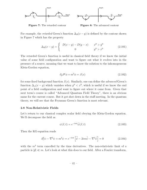
Im(p 0)Im(p 0)−E p+ E pRe(p 0)−E p+E pRe(p 0)Figure 7: The retarded contourFigure 8: The advanced contourFor example, the retarded Green’s function ∆ R (x − y) is defined by the contour shownin Figure 7 which has the property∆ R (x − y) ={D(x − y) − D(y − x) x 0 > y 00 y 0 > x 0 (2.101)The retarded Green’s function is useful in classical field theory if we know the initialvalue of some field configuration and want to figure out what it evolves into in thepresence of a source, meaning that we want to know the solution to the inhomogeneousKlein-Gordon equation,∂ µ ∂ µ φ + m 2 φ = J(x) (2.102)for some fixed background function J(x). Similarly, one can define the advanced Green’sfunction ∆ A (x − y) which vanishes when y 0 < x 0 , which is useful if we know the endpoint of a field configuration and want to figure out where it came from. Given thatnext term’s course is called “Advanced Quantum Field Theory”, there is an obviousname for the current course. But it got shot down in the staff meeting. In the quantumtheory, we will see that the Feynman Green’s function is most relevant.2.8 Non-Relativistic FieldsLet’s return to our classical complex scalar field obeying the Klein-Gordon equation.We’ll decompose the field asThen the KG-equation readsψ(⃗x, t) = e −imt ˜ψ(⃗x, t) (2.103)]∂t 2 ψ − ∇2 ψ + m 2 ψ = e[¨˜ψ −imt − 2im ˙˜ψ − ∇2 ˜ψ = 0 (2.104)with the m 2 term cancelled by the time derivatives. The non-relativistic limit of aparticle is |⃗p| ≪ m. Let’s look at what this does to our field. After a Fourier transform,– 41 –