Quantum Field Theory

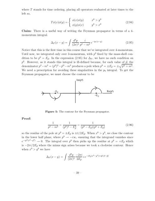
where T stands for time ordering, placing all operators evaluated at later times to theleft so,{φ(x)φ(y) x 0 > y 0Tφ(x)φ(y) =(2.94)φ(y)φ(x) y 0 > x 0Claim: There is a useful way of writing the Feynman propagator in terms of a 4-momentum integral.∫d 4 p i∆ F (x − y) =e−ip·(x−y) (2.95)(2π) 4 p 2 − m 2Notice that this is the first time in this course that we’ve integrated over 4-momentum.Until now, we integrated only over 3-momentum, with p 0 fixed by the mass-shell conditionto be p 0 = E ⃗p . In the expression (2.95) for ∆ F , we have no such condition onp 0 . However, as it stands this integral is ill-defined because, for each value of ⃗p, thedenominator p 2 −m 2 = (p 0 ) 2 −⃗p 2 −m 2 produces a pole when p 0 = ±E ⃗p = ± √ ⃗p 2 + m 2 .We need a prescription for avoiding these singularities in the p 0 integral. To get theFeynman propagator, we must choose the contour to beIm(p 0)−E p+ E pRe(p 0)Proof:Figure 5: The contour for the Feynman propagator.1p 2 − m = 12 (p 0 ) 2 − E⃗p2=1(p 0 − E ⃗p )(p 0 + E ⃗p )(2.96)so the residue of the pole at p 0 = ±E ⃗p is ±1/2E ⃗p . When x 0 > y 0 , we close the contourin the lower half plane, where p 0 → −i∞, ensuring that the integrand vanishes sincee −ip0 (x 0 −y 0) → 0. The integral over p 0 then picks up the residue at p 0 = +E ⃗p whichis −2πi/2E ⃗p where the minus sign arises because we took a clockwise contour. Hencewhen x 0 > y 0 we have∫∆ F (x − y) =d 3 p(2π) 4 −2πi2E ⃗pi e −iE ⃗p(x 0 −y 0 )+i⃗p·(⃗x−⃗y)– 39 –