Quantum Field Theory

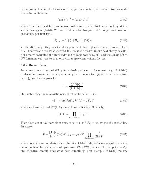
is the probability for the transition to happen in infinite time t → ∞. We can writethe delta-functions as(2π) 2 δ(ω) 2 = (2π)δ(ω) T (3.82)where T is shorthand for t → ∞ (we used a very similar trick when looking at thevacuum energy in (2.25)). We now divide out by this power of T to get the transitionprobability per unit time,˙ P n→m = 2π| 〈m| H int |n〉 | 2 δ(ω) (3.83)which, after integrating over the density of final states, gives us back Fermi’s Goldenrule. The reason that we’ve stressed this point is because, in our field theory calculations,we’ve computed the amplitudes in the same way as (3.81), and the square of theδ (4) -functions will just be re-interpreted as spacetime volume factors.3.6.2 Decay RatesLet’s now look at the probability for a single particle |i〉 of momentum p I (I=initial)to decay into some number of particles |f〉 with momentum p i and total momentump F = ∑ i p i. This is given byP =| 〈f|S |i〉 |2〈f|f〉 〈i| i〉(3.84)Our states obey the relativistic normalization formula (2.65),〈i|i〉 = (2π) 3 2E ⃗pI δ (3) (0) = 2E ⃗pI V (3.85)where we have replaced δ (3) (0) by the volume of 3-space. Similarly,〈f|f〉 =∏2E ⃗pi V (3.86)final statesIf we place our initial particle at rest, so ⃗p I = 0 and E ⃗pI = m, we get the probabilityfor decayP = |A fi| 22mV (2π)4 δ (4) (p I − p F ) V T∏final states12E ⃗pi V(3.87)where, as in the second derivation of Fermi’s Golden Rule, we’ve exchanged one of thedelta-functions for the volume of spacetime: (2π) 4 δ (4) (0) = V T. The amplitudes A fiare, of course, exactly what we’ve been computing. (For example, in (3.30), we saw– 73 –