Magazine – PDF - Cal Lab Magazine

METROLOGY 101: VERIFYING 1 MW 50 MHZ POWER REFERENCE OUTPUT SWR2013JANUARYFEBRUARYMARCHStating Best Uncertainties Over aRange of ValuesAn Uncertainty Analysis for a PositiveDisplacement Liquid Flow CalibratorUsing the Water Draw Technique

Transient GeneratorsRFI/EMI/EMCDC Power SuppliesVXISynthesizersElectronic LoadsSignal GeneratorsSpectrum AnalyzersDigital MultimetersArbitrary Waveform GeneratorsCurve TracersGround BondESD TestCalibratorsSemiconductor Testers Bio-Medical TestFunction Generators Megohmmeters Data Aquisition PXICommunication Analyzers LCR Meters Sweep GeneratorsNetwork AnalyzersAC Power SourcesNoise MeasuringOscilloscopesVector Signal GeneratorsPulse Generators Logic Analyzers Modulation AnalyzersImpedance Analyzers Tracking Generators Frequency CountersService MonitorsCable Locators Pattern GeneratorsHipot TestersLightwavePower MetersVNAAudio AnalyzersAviation TestAmplifiersRepair Support For More Than 10,000 Different Test Equipment ProductsLegacy & Current Product Repair SupportEnd-Of-Support (EOS) Repair ProgramsFast, Simple Online Order Creation (RMA)Account Historical Data & Reporting ToolsSingle–Incident Repair SupportMulti-Year Repair AgreementsPost-Repair Calibration AvailableISO 17025:2005 Accredited CalibrationTest Equipment Repair Corporation – Industry’s Source For RepairToll Free: (866) 965-4660customerservice@testequipmentrepair.com5965 Shiloh Rd E.Alpharetta, GA 30005

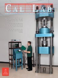
Volume 20, Number 1www.callabmag.comFEATURES20 Metrology 101: Verifying 1 mW 50 MHz Power Reference OutputStanding Wave Ratio (SWR)Charles Sperrazza24 Stating Best Uncertainties Over a Range of ValuesDavid Deaver31 An Uncertainty Analysis for a Positive Displacement LiquidFlow Calibrator Using the Water Draw TechniqueWesley B. EnglandDEPARTMENTS2 Calendar3 Editor’s Desk11 Industry and Research News15 New Products and Services44 Classifieds44 Cal-Toons by Ted GreenON THE COVER: Micah McDonald is preparing to Cross-Float a customer’s Ametek deadweight tester against Alaska Metrology &Calibration Services’ Ruska 2485 deadweight tester. Micah is performing this work in a Mobile Calibration Laboratory performingon-site work for BP Exploration and ConocoPhillips in Prudhoe Bay, Alaska.Jan • Feb • Mar 20131Cal Lab: The International Journal of Metrology

CALENDARCONFERENCES & MEETINGS 2013Mar 3-4 Southeast Asia Flow Measurement Conference. KualaLumpur, Malaysia. http://www.tuvnel.com.Mar 7-8 METROMEET – 9th International Conference onIndustrial Dimensional Metrology. Bilboa, Spain. METROMEETsummons international leaders of the sector, to expose thelatest advances in the subject and to propose product qualityimprovements and production efficiency. http://www.metromeet.org.Mar 18-22 Measurement Science Conference (MSC). Anaheim,CA. This year’s theme is “Global Economic Challenges DriveOperational Change In Metrology.” Take your knowledge to thenext level at our annual user conference and join over a thousandMSC users from all over the world for five days of education fromover 30 developers and sessions. http://www.msc-conf.com.Apr 22-25 FORUMESURE. Casablanca, Morocco. This exhibitionand technical workshops on Measurement and Quality, organizedby The African Committee of Metrology (CAFMET), bringstogether industries in the search for process control measurement,testing and analysis to ensure quality products and services. http://www.forumesure.com.Apr 29-May 2 ESTECH. San Diego, CA. ESTECH 2013, the 59thannual technical conference of the Institute of EnvironmentalSciences and Technology (IEST), provides a platform for nationaland international professionals to share crucial strategies, research,and best practices for a wide range of Contamination Control,Test and Reliability, and Nanotechnology applications. http://www.iest.org.Jul 14-18 NCSL International. Nashville, TN. The theme for the2013 NCSLI Workshop & Symposium is “Metrology in a Fast PacedSociety,” http://ncsli.org.Jul 18-19 IMEKO/TC-4 Symposium. Barcelona, Spain. The 17thTC-4 Workshop IWADC on ADC and DAC Modeling and Testingwill take place during the 19th IMEKO TC-4 Symposium onMeasurements of Electrical Quantities. http://www.imeko2013.es/.Sep 24-26 The 16th International Flow Measurement Conference(FLOMEKO). Paris, France. Flomeko 2013 will provide the perfectopportunity for practitioners of metrology from a wide variety ofindustries to exchange ideas with researchers, national laboratoriesand academics and to explain just how new and improvedmetrology can play a vital part in all their activities. http://www.flomeko2013.fr/.IAS Laboratory Accreditationto ISO/IEC Standard 17025The International Accreditation Service (IAS)offers laboratories Accreditation Service Plus++ Quick scheduling and efficient assessments+ On demand responsiveness+ True affordability+ Global recognition by ILAC+ Proof of compliance with ISO/IEC 17025Learn about the Benefits of IAS Accreditationwww.iasonline.org/ca866-427-442211-05610Cal Lab: The International Journal of Metrology2 Jan • Feb • Mar 2013

EDITOR’S DESKPUBLISHERMICHAEL L. SCHWARTZEDITORSITA P. SCHWARTZCAL LABPO Box 111113Aurora, CO 80042TEL 303-317-6670 • FAX 303-317-5295office@callabmag.comwww.callabmag.comEDITORIAL ADVISORSCAROL L. SINGERJAY BUCHERBUCHERVIEW METROLOGYCHRISTOPHER L. GRACHANENHEWLETT-PACKARDMIKE SURACICONSULTANTLOCKHEED MISSILES & SPACE (RETIRED)LEAD ASSESSOR, A2LA (RETIRED)MARTIN DE GROOTMARTINDEGROOT CONSULTANCYSubscription fees for 1 year (4 issues)$50 for USA, $55 Mexico/Canada,$65 all other countries.Visit www.callabmag.comto subscribe.Printed in the USA.© Copyright 2013 CAL LAB.ISSN No. 1095-4791Many ThanksWe’ve fallen off the proverbial economic cliff, but the car still reluctantlyfires up at five degrees and the house roof is still solid… the world did notend. In fact, the church across the street is still rocking on Wednesday nightsand “Junior,” the neighborhood skunk, has returned now twice as big.Since life progresses as usual, I took upon myself to clean up our mailing listfor undeliverable addresses and those who may not want to keep receiving themagazine. We source our mailing list from the MSC and NCSLI conferences,as well as paid subscriptions. We would love to send complimentarysubscriptions forever, but eventually we have to ask if subscribers wouldbe willing to pay for their subscriptions if they are no longer attending theconferences.We decided to keep subscription rates static indefinitely and offer a 10%discount to those who sign up for two years in order to attract more payingsubscriptions. Because of the increasing rise of printing and postage costs,advertising revenue is not always enough to keep publications continuingtoday. So I would like to especially thank all those who contribute to CalLab Magazine in order to keep us printing—article contributors; Ted Green,the creator of Cal-Toons; advertisers (hoorah advertisers!); subscribers; andpeers and community members who provide us with valuable feedback andsuggestions… many, many thanks.For this issue, our Metrology 101 contributor is Charles Sperrazza ofTegam, who wrote about verification of the Standing Wave Ratio (SWR) of a50 MHz reference. David Deaver contributed a great paper on “Stating BestUncertainties Over a Range of Values,” and Wesley England contributed hispaper, “An Uncertainty Analysis for a Positive Displacement Liquid FlowCalibrator Using the Water Draw Technique,” which was awarded Best Paperat MSC 2011.Again, thank you to everyone who makes it possible to print Cal LabMagazine each quarter!Regards,Sita SchwartzJan • Feb • Mar 20133Cal Lab: The International Journal of Metrology

CALENDARSEMINARS: Online & Independent StudyASQ CCT (Certified Calibration Technician) Exam PreparationProgram. Learning Measure. http://www.learningmeasure.com/.AC-DC Metrology– Self-Paced Online Training. Fluke Training.http://us.flukecal.com/training/courses.Basic Measurement Concepts Program. Learning Measure. http://www.learningmeasure.com/.Basic Measuring Tools – Self Directed Learning. The QC Group,http://www.qcgroup.com/sdl/.Basic RF and Microwave Program. Learning Measure. http://www.learningmeasure.com/.Certified Calibration Technician – Self-study Course. J&GTechnology. http://www.jg-technology.com/selfstudy.html.Introduction to Measurement and Calibration – Online Training.The QC Group, http://www.qcgroup.com/online/.Intro to Measurement and Calibration – Self-Paced OnlineTraining. Fluke Training. http://us.flukecal.com/training/courses.ISO/IEC 17025 Accreditation Courses. WorkPlace Training, http://www.wptraining.com/.Measurement Uncertainty – Self-Paced Online Training. FlukeTraining. http://us.flukecal.com/training/courses.Measurement Uncertainty Analysis – Online Training. The QCGroup, http://www.qcgroup.com/online/.Metrology for Cal Lab Personnel– Self-Paced Online Training.Fluke Training. http://us.flukecal.com/training/courses.Metrology Concepts. QUAMETEC Institute of MeasurementTechnology. http://www.QIMTonline.com.Precision Dimensional Measurement – Online Training. The QCGroup, http://www.qcgroup.com/online/.Precision Measurement Series Level 1 & 2. WorkPlace Training,http://www.wptraining.com/.Precision Electrical Measurement – Self-Paced Online Training.Fluke Training. http://us.flukecal.com/training/courses.Vibration and Shock Testing. Equipment Reliability Institute,http://www.equipment-reliability.com/distance_learning.html.The Uncertainty Analysis Program. Learning Measure. http://www.learningmeasure.com/.Work fasterand smarterwith newMET/TEAM softwareMET/TEAM Test Equipment AssetManagement software makes it easyto consistently track, manage andreport on all aspects of your calibrationoperations and comply with regulatorystandards. Fully integrates with MET/CAL ®calibration software and optional mobile,commerce, and customer portal modulesto help you manage more workloadwith less work.Field calibrationQuality/lab managementCustomer serviceMET/TEAMSoftwareTMLab calibrationSystem and databaseadministrationAsset trackingand managementGet the details: www.flukecal.com/GoTEAMFluke Calibration. Precision, performance, confidence.Electrical RF Temperature Pressure Flow Software©2012 Fluke Calibration. Specifications are subject to change without notice. Ad 4225447A_EN4225447A_EN_MET_TEAM_half_Cal_Lab.indd 110/11/12 1:39 PMCal Lab: The International Journal of Metrology4 Jan • Feb • Mar 2013

Magnetic Field MeasurementFluxgate TransducersHigh Sensitivity for Low FieldsOne and Three-axis Transducers with ±10V (±3V Mag640) analogoutputs for each axis. For environmental field monitoring,mapping and active cancellation. Cryogenic sensors available.Field Ranges 70, 100, 250, 500, 1000μTFrequency Response dc to 3kHz (-3dB) (Mag03),dc to >1kHz (Mag690, Mag649)Noise Level< 20pTrms/√Hz at 1Hz (Mag690),< 10pTrms/√Hz at 1Hz (Mag649),< 12pTrms/√Hz at 1Hz (Mag03 standard),< 6pTrms/√Hz at 1Hz (Mag03 low noise),Mag648/649Mag690Mag-03MSMag-03MCHall TransducersAnalog Output for Mapping or ControlOne-, Two- and Three-axis Transducers with ±10V analogoutputs for each axis.Field RangesAccuracy ±1% or ±0.1%Frequency Response20mT, 200mT, 2T, 5T, 10T, 20Tdc to 2.5kHz (-3dB); Special to 25kHzWhite Noise at >10Hz 0.12μT/√Hz for 2T range (Y-axis),2μT/√Hz for 2T range (3-axis)Hall Transducer Probe PackagesPackage“A”5mmPackage“B”4mmPackage“G”2mmPackage“E”0.64mmUSB/Handheld TeslametersUSB Connector, 3-Axis, Handheld PDA AvailableFor pre-installation site surveys for magnetically sensitive equipment.Post-installation surveys of the dc and ac fringe fields of large magnetsand magnetic assemblies. Field harmonic measurements over time fornon-invasive load and condition monitoring of ac power assemblieslike tranformers and motors.Fluxgate ProbeField RangeNoiseTFM1186100μT5nT p-p, 8 nT RMS (2kSPS, no averaging);4nT p-p (100x averaging)Hall Probe THM1186-LF THM1186-HFField Ranges 8mT 0.1T, 0.5T, 3T, 20TResolution 2μT 3mTon 3TrangeNMR TeslameterMapping and Calibration StandardFor field calibration, mapping and control with high resolution,very highstability and absolute accuracy.Field Ranges from 0.04T to 13.7TResolutionAbsolute Accuracy±0.1μT or 1Hz (proton sample)±5ppmRS-232C and IEEE-488 InterfacesMultiprobe NMR arrays for precision mapping of large magnetsTFM1186Fluxgate ProbeTHM1176Hall ProbePT2025GMW Associates • www.gmw.com

CALENDARSEMINARS: DimensionalFeb 28-Mar 1 Seminar – Gage Calibration Systems and Methods.Aurora, IL. The Mitutoyo Institute of Metrology. http://www.mitutoyo.com.Mar 7-8 Hands-On Gage Calibration and Repair Workshop.Minnetonka, MN. http://www.iicttraining.com.Mar 12-13 Seminar – Dimensional Metrology: Applicationsand Techniques. City of Industry, CA. The Mitutoyo Institute ofMetrology. http://www.mitutoyo.com.Mar 19-20 Hands-On Gage Calibration and Repair Workshop.Houston, TX. http://www.iicttraining.com.Mar 19-21 Gage Calibration and Minor Repair Training.Cincinnati, OH. Cincinnati Precision Instruments,Inc. http://www.cpi1stop.com/.Mar 27-28 Hands-On Gage Calibration and Repair Workshop.Cincinnati, OH. http://www.iicttraining.com.Apr 4-5 Hands-On Gage Calibration and Repair Workshop.Billings, MT. http://www.iicttraining.com.Cal Lab Mag 6.5x4.75_2012 5/23/12 2:36 PM Page 1Apr 8-9 Hands-On Gage Calibration and Repair Workshop.Portland, OR. http://www.iicttraining.com.Apr 9-11 Seminar - Hands-On Gage Calibration. Elk GroveVillage, IL. The Mitutoyo Institute of Metrology. http://www.mitutoyo.com.May 14-16 Gage Calibration and Minor Repair Training.Cincinnati, OH. Cincinnati Precision Instruments,Inc. http://www.cpi1stop.com/.Jun 18-20 Gage Calibration and Minor Repair Training.Cincinnati, OH. Cincinnati Precision Instruments,Inc. http://www.cpi1stop.com/.SEMINARS: ElectricalMar 7-8 Essential Electrical Metrology. Orlando, FL. WorkPlaceTraining. http://www.wptraining.com.Apr 8-11 MET-301 Advanced Hands-on Metrology. Seattle,WA. Fluke Calibration. http://us.flukecal.com/training/courses/MET-301.Jun 3-6 MET-101 Basic Hands-on Metrology. Everett, WA. FlukeCalibration. http://us.flukecal.com/training/courses/MET-101.On-site calibration and adjustment.HygroGen2• Generates stable humidity and temperature conditions• Increased calibration productivity• Stable humidity values within 5 to 10 minutes• Calibrates up to 5 sensors simultaneously• Integrated sample loop for use with Reference Hygrometers• Integrated desiccant cell and digital water level monitoring• Easy-to-use graphical user interfaceVisit www.rotronic-usa.com for more information or call 631-427-3898.ROTRONIC Instrument Corp, 135 Engineers Road, Hauppauge, NY 11788, USA, sales@rotronic-usa.comCal Lab: The International Journal of Metrology6 Jan • Feb • Mar 2013

CALENDARSEMINARS: Flow & PressureFeb 25-Mar 1 Principles of Pressure Calibration. Phoenix, AZ.Fluke Calibration. http://us.flukecal.com/Principles-of-Pressure.Mar 6-7 Fundamentals of Ultrasonic Flowmeters TrainingCourse. Brisbane, Australia. http://www.ceesi.com.Mar 18-19 NIST Pressure and Vacuum Measurement. Anaheim,CA. NIST Seminar N03, hosted by MSC. http://www.msc-conf.com.Mar 26-27 Fundamentals of Ultrasonic Flowmeters TrainingCourse. Houston, TX. http://www.ceesi.com.Apr 15-19 Advanced Piston Gauge Metrology. Phoenix, AZ.Fluke Calibration. http://us.flukecal.com/Advanced-Piston-Gauge.Apr 16-18 European Ultrasonic Meter User’s Workshop. Lisbon,Portugal. http://www.ceesi.com.May 14-16 Principles and Practice of Flow Measurement TrainingCourse. East Kilbride, UK. http://www.tuvnel.com/tuvnel/courses_workshops_seminars/.SEMINARS: GeneralMar 4-6 Cal Lab Training; Beyond 17025. Orlando, FL. WorkPlaceTraining http://www.wptraining.com.Mar 25-27 Instrumentation for Test and Measurement. Las Vegas,NV. Technology Training, Inc. http:// www.ttiedu.com.May 20-23 CLM-303 Effective Cal Lab Management. Everett, WA.http://us.flukecal.com/lab_management_training.Apr 8-12 Calibration Lab Operations / Understanding ISO 17025.Las Vegas, NV. Technology Training Inc. http://www.ttiedu.com.Apr 15 Fundamentals of Metrology. Gaithersburg, MD. http://www.nist.gov/pml/wmd/labmetrology/training.cfm.SEMINARS: Mass & WeightMar 4 Mass Metrology Seminar. Gaithersburg, MD. http://www.nist.gov/pml/wmd/labmetrology/training.cfm.May 13 Mass Metrology Seminar. Gaithersburg, MD. http://www.nist.gov/pml/wmd/labmetrology/training.cfm.HIGH VOLTAGECALIBRATION LABCustom Design is our Specialty!DESIGN, MANUFACTURE, TEST &CALIBRATE:• HV VOLTAGE DIVIDERS• HV PROBES• HV RELAYS• HV AC & DC HIPOTS• HV DIGITAL VOLTMETERS• HV CONTACTORS• HV CIRCUIT BREAKERS• HV RESISTIVE LOADS• SPARK GAPS• FIBER OPTIC SYSTEMSISO/IEC 17025:2005CALIBRATION CERT #2746.01ISO 9001:2008QMS CERTIFIEDHV LAB CALIBRATION CAPABILITIES:• UP TO 450kV PEAK 60Hz• UP TO 400kV DC• UP TO 400kV 1.2x50μSLIGHTNING IMPULSEHV LAB CALIBRATION STANDARDSISO/IEC 17025:2005 ACCREDITEDISO 9001:2008 QMS CERTIFIEDN.I.S.T. TRACEABILITYN.R.C. TRACEABILITYHigh Voltage Dividers & ProbesROSS ENGINEERING CORPORATION540 Westchester Dr. Campbell, CA 95008www.rossengineeringcorp.com408-377-4621±Jan • Feb • Mar 20137Cal Lab: The International Journal of Metrology

CALENDARSEMINARS: Measurement UncertaintyMar 12-13 Estimating Measurement Uncertainty. Aurora, IL.The Mitutoyo Institute of Metrology. http://www.mitutoyo.com.Mar 18-19 JCGM Guide to the Expression of UncertaintyMeasurement. Anaheim, CA. NIST Seminar N04, hosted by MSC.http://www.msc-conf.com.Mar 20-22 Measurement Uncertainty Workshop. Fenton, MI.QUAMETEC Institute of Measurement Technology. http:// www.QIMTonline.com.May 7-9 MET-302 Introduction to Measurement Uncertainty.Everett, WA. Fluke Calibration. http://us.flukecal.com/training/courses/MET-302.May 15-17 Measurement Uncertainty Workshop. Fenton, MI.QUAMETEC Institute of Measurement Technology. http:// www.QIMTonline.com.SEMINARS: StandardsMar 18-19 The ISO/IEC 17025 Accreditation Process. Anaheim,CA. NIST Seminar N01, hosted by MSC. http://www.msc-conf.com.SEMINARS: TemperatureMar 5-7 Infrared Temperature Metrology. American Fork, UT.Fluke Calibration, http://us.flukecal.com/tempcal_training.Mar 18-20 Selection, Calibration, and Use of ContactThermometers. Anaheim, CA. NIST Seminar N02, hosted byMSC. http://www.msc-conf.com.Jun 11-13 Principles of Temperature Metrology. Everett, WA.Fluke Calibration. http://us.flukecal.com/training/courses/Principles-Temperature-Metrology.SEMINARS: VibrationMar 5-7 Fundamentals of Random Vibration and Shock Testing.Houston, TX. http://www.equipment-reliability.com.Mar 11-14 Mechanical Shock and Modal Test Techniques. LasVegas, NV. Technology Training, Inc. http://www.ttiedu.com.Apr 9-11 Fundamentals of Random Vibration and ShockTesting, HALT, ESS, HASS (...). College Park MD. http://www.equipment-reliability.com.Force and Torque Calibration ServiceLower your test uncertainty ratios by having instrumentscalibrated at a more precise level of measurement certainty: Primary Force and Torque standards accurate to0.002% of applied for most capacities Hassle-Free Calibration Service - Morehousedoes not require RMAʼs and works extensivelyto ensure calibrations are performed in a mannerthat replicates how the instruments are used Force Calibration performed in our laboratory to2,250,000 lbf in compression and 1,200,000 lbfin tension and equivalent SI units Torque Calibration performed in our laboratoryto 1475 ft - lbf and equivalent SI units Calibrations performed in accordance withcustomer specifications, ASTM E74, ISO 376,ASTM E 2428 and BS 7882ISO 17025 AccreditedAmerican Association of LaboratoryAccreditation Calibration Cert 1398.01Prompt Delivery of 5-7 Days on Most Items. Expedited Service AvailableMOREHOUSE FORCE & TORQUE CALIBRATION LABORATORIESPhone: 717-843-0081 / Fax: 717-846-4193 / www.mhforce.com / e-mail: hzumbrun@mhforce.comINSTRUMENT COMPANY, INC.1742 Sixth Avenue ¥ York, PA USACal Lab: The International Journal of Metrology8 Jan • Feb • Mar 2013

Since elementary school, you’ve hadto show your work. Make sure yourcalibration provider does too.When it comes to calibration, a simplepass/fail answer isn’t enough. You need afull report of tests conducted — includingaccuracy. And if the test results were out ofspec, how far? A certifi cate alone is not theanswer to calibration. Ask to see the work.Understand more aboutcalibration. Scan or visithttp://qrs.ly/2y2kkcofor videos.Not all calibrations are created equal,see why “the work” matters:www.agilent.com/find/SeeTheWork© Agilent Technologies, Inc. 2013 u.s. 1-800-829-4444 canada: 1-877-894-4414

© 2012 Lockheed Martin CorporationMISSION SUCCESSIS OFTEN MEASURED IN PARTS-PER-MILLIONLockheed Martin Calibration Services. Comprehensive, affordable, highly accuratecalibration support. Delivered by our experts with precision and care for 30 years.ISO/IEC 17025:2005 Accreditation, A2LA 2258.011-800-275-3488www.lockheedmartin.com/calibration

INDUSTRY AND RESEARCH NEWSCarl Zeiss Industrial MetrologyAcquires HGV VosselerWith the acquisition of HGV Vosseler GmbH & Co. KG inÖhringen, Germany, Carl Zeiss Industrial Metrology (IMT) isstrengthening its presence in the market for process controland inspection in car making.HGV is one of the world’s three leading companies for 3Dinline measuring solutions based on optical 3D measuringtechnology on robots which are primarily used for car bodyinspection directly on the production line in the automotiveindustry. Robot-assisted inline measuring technology for carbodies is an important addition to metrology in the measuringlab. In addition to 3D inline measuring technology, HGValso offers innovative optical image processing systems forquality inspection.Effective immediately, Dr. Kai-Udo Modrich will beresponsible for the new company, Carl Zeiss MachineVision GmbH & Co KG. Under the ZEISS brand, the approx.60 employees in Öhringen, Germany, will have futureperspectives focused on further growth.You can find further info here: http://www.zeiss.de/press/pr003cd603.Transcat Acquisition of Cal-Matrix Metrology Inc.Transcat, Inc., a leading distributor of professional gradehandheld test, measurement and control instruments andaccredited provider of calibration, repair, inspection andother compliance services, announced today that it hasacquired Cal-Matrix Metrology Inc., a leading Canadianprovider of commercial and accredited calibrations andcoordinate measurement inspection services. Headquarteredin Burlington (Greater Toronto Area), the acquisition greatlyexpands Transcat’s presence in Southern Ontario, the largestmarket in Canada, and adds a lab in Montreal, Quebec.Cal-Matrix offers calibration services to clients who requirecalibration of their RF, DC low frequency, optics, mechanical,torque and pressure measurement equipment. Cal-Matrixmaintains a comprehensive ISO/IEC-17025-2005 certifiedscope for calibration and coordinate measurement inspection.Lee Rudow, President and Chief Operating Officer ofTranscat, added, “In order to continue this superior levelof customer service, Cal-Matrix’s management team and itsnearly 30 employees have been retained by Transcat.”More information about Transcat can be found on itswebsite at: transcat.com.Jan • Feb • Mar 201311Cal Lab: The International Journal of Metrology

INDUSTRY AND RESEARCH NEWSNIST’s ‘Nanotubes on a Chip’ May SimplifyOptical Power MeasurementsThe National Institute of Standards and Technology(NIST) has demonstrated a novel chip-scale instrumentmade of carbon nanotubes that may simplify absolutemeasurements of laser power, especially the light signalstransmitted by optical fibers in telecommunicationsnetworks.The prototype device, a miniature version of aninstrument called a cryogenic radiometer, is a silicon chiptopped with circular mats of carbon nanotubes standing onend.* The mini-radiometer builds on NIST’s previous workusing nanotubes, the world’s darkest known substance,to make an ultraefficient, highly accurate optical powerdetector,** and advances NIST’s ability to measure laserpower delivered through fiber for calibration customers.***“This is our play for leadership in laser powermeasurements,” project leader John Lehman says. “Thisis arguably the coolest thing we’ve done with carbonnanotubes. They’re not just black, but they also have thetemperature properties needed to make components likeelectrical heaters truly multifunctional.”NIST and other national metrology institutes around theworld measure laser power by tracing it to fundamentalelectrical units. Radiometers absorb energy from lightand convert it to heat. Then the electrical power needed tocause the same temperature increase is measured. NISTresearchers found that the mini-radiometer accuratelymeasures both laser power (brought to it by an opticalfiber) and the equivalent electrical power within thelimitations of the imperfect experimental setup. The testswere performed at a temperature of 3.9 K, using light atthe telecom wavelength of 1550 nanometers.The tiny circular forests of tall, thin nanotubes calledVANTAs (“vertically aligned nanotube arrays”) haveseveral desirable properties. Most importantly, theyuniformly absorb light over a broad range of wavelengthsand their electrical resistance depends on temperature. Theversatile nanotubes perform three different functions in theradiometer. One VANTA mat serves as both a light absorberand an electrical heater, and a second VANTA mat servesas a thermistor (a component whose electrical resistancevaries with temperature). The VANTA mats are grown onthe micro-machined silicon chip, an instrument design thatis easy to modify and duplicate. In this application, thewww.entegra-corp.com240-672-7645Providing Reference Pulse Generators for Oscilloscope CalibrationsEntegra’s Pulse Generators:Models available for calibrating the step response of 12 GHz,20 GHz, and 50 GHz bandwidth oscilloscopesTransition durations down to 9 ps (10 % - 90 %) and both thepositive and negative transitions are fast550 mV step amplitude typicalDifferential output model availableCal Lab: The International Journal of Metrology12 Jan • Feb • Mar 2013

INDUSTRY AND RESEARCH NEWSindividual nanotubes are about 10 nanometers in diameterand 150 micrometers long.By contrast, ordinary cryogenic radiometers use moretypes of materials and are more difficult to make. Theyare typically hand assembled using a cavity painted withcarbon as the light absorber, an electrical wire as the heater,and a semiconductor as the thermistor. Furthermore,these instruments need to be modeled and characterizedextensively to adjust their sensitivity, whereas theequivalent capability in NIST’s mini-radiometer is easilypatterned in the silicon.NIST plans to apply for a patent on the chip-scaleradiometer. Simple changes such as improved temperaturestability are expected to greatly improve deviceperformance. Future research may also address extendingthe laser power range into the far infrared, and integrationof the radiometer into a potential multipurpose “NIST ona chip” device.* N.A. Tomlin, J.H. Lehman. Carbon nanotube electricalsubstitutioncryogenic radiometer: initial results. OpticsLetters. Vol. 38, No. 2. Jan. 15, 2013.** See 2010 NIST Tech Beat article, “Extreme Darkness:Carbon Nanotube Forest Covers NIST’s Ultra-darkDetector,” at www.nist.gov/pml/div686/dark_081710.cfm.OHMLABSresistorsAD3.10_Layout 1 4/8/10 12:46 PM Page 1***See 2011 NIST Tech Beat article, “Prototype NISTDevice Measures Absolute Optical Power in Fiberat Nanowatt Levels,” at www.nist.gov/pml/div686/radiometer-122011.cfm.Source: NIST Tech Beat, January 24, 2013.Image Source: National Institute of Standards andTechnology. Credit: Tomlin/NIST.HIGH RESISTANCE STANDARDS• FULLY GUARDED FOR ANY RATIO• BPO OR N TYPE CONNECTORS• VERY LOW TCR & VCR• STABLE OVER TIME• INTERNAL TEMPERATURE SENSOR• 17025 ACCREDITED CALIBRATIONMODEL RESISTANCE TCR / VCR106 1 MΩ < 1 / < 0.1107 10 MΩ < 3 / < 0.1108 100 MΩ < 10 / < 0.1109 1 GΩ < 15 / < 0.1110 10 GΩ < 20 / < 0.1111 100 GΩ < 30 / < 0.1112 1 TΩ < 50 / < 0.1113 10 TΩ < 300 / < 0.1SEE WWW.OHM-LABS.COM FOR SPECIFICATIONS611 E. CARSON ST. PITTSBURGH, PA 15203TEL 412-431-0640 FAX 412-431-0649WWW.OHM-LABS.COMJan • Feb • Mar 201313Cal Lab: The International Journal of Metrology

SOLUTIONSFusing Software With MetrologyMET/CAL ®MUDCATSAUTOMATIONINCREASESEFFICIENCYPS-CAL ®.NETWEB TOOLSBetter, cheaper, and faster is the name of the gamewhen it comes to calibration. Whether you’re abig lab, small lab, internal or third party, youhave to increase your accuracy, productivity andrepeatability on a limited budget.Cal Lab Solutions is your technology partner and wehelp labs around the world increase their efficiency.Our engineers are experts in automation technologiesand know how to apply these technologies to makeyour lab more efficient and productive, withoutbreaking the bank.For more information on what we do, and how wedo it, visit us online at www.callabsolutions.com, orcall us at 303-317-6670.PO Box 111113 • Aurora, Colorado 80042 • USATelephone 303.317.6670 • Facsimile 303.317.5295 • sales@callabsolutions.com

NEW PRODUCTS AND SERVICESAgilent InfiniiVision 4000 X-SeriesOscilloscopeAgilent Technologies Inc. introducesthe groundbreaking InfiniiVision 4000X-Series digital-storage and mixed-signaloscilloscopes. This new series establishesunprecedented levels of flexibility and easeof use among units that use an embeddedoperating system.The new lineup offers bandwidthsfrom 200 MHz to 1.5 GHz and severalbenchmark features. First is an industryleadingupdate rate of 1 million waveformsper second with standard segmentedmemory, which uses patented MegaZoomIV smart memory technology. Next area 12-inch capacitive touch screen-theindustry’s largest-and the exclusive, allnewInfiniiScan Zone touch-triggeringcapability. Because the 4000 X-Series wasdesigned specifically for touch operation,engineers can select targets naturally andquickly. For example, InfiniiScan Zonemakes triggering as easy as finding thesignal of interest and drawing a box aroundit: If users can see a signal, they can triggeron it.The high level of integration starts withthe capabilities of five instruments on oneunit: oscilloscope, digital channels (MSO),protocol analysis, digital voltmeter anddual-channel WaveGen function/arbitrarywaveform generator. The 4000 X-Seriesalso supports a wide range of popularoptional applications: MIL-STD 1553and ARINC 429; I2S; CAN/LIN; FlexRay;RS232/422/485/UART; I2C/ SPI; and USB2.0 Hi-Speed, Full-Speed and Low-Speedtriggering and analysis (the first hardwarebasedUSB trigger/decode oscilloscopesolution).The InfiniiVision 4000 X-Series includes200-MHz, 350-MHz, 500-MHz, 1-GHzand 1.5-GHz models. The standardconfiguration for all models includes 4Mpts of memory and segmented memory.Information about the InfiniiVision 4000X-Series oscilloscopes is available at www.agilent.com/find/4000X-Series.Symmetricom 3120A Test ProbeSymmetricom®, Inc., a worldwideleader in precision time andfrequency technologies, announcedthe launch of a new high-performance,low-cost measurement solution,the Symmetricom 3120A PhaseNoise Test Probe. The latest additionto Symmetricom’s state-of-the-art timingtest set portfolio, the 3120A Test Probecomes in a convenient small form factorand measures Phase Noise and AllanDeviation as part of the base hardware kit.Additional software options are availableto measure AM noise floor and signalstatistics such as HDEV, TDEV, MDEV andjitter, and for use as a frequency counterand for mask testing.Unlike traditional solutions thatare desktop-bound due to size andweight, Symmetricom’s 3120A Test Probeis small enough to be carried around fromlocation-to-location, and inexpensiveenough to have at each bench. Whetherused on a busy manufacturing floor, ina tight server closet or in R&D labs, the3120A helps characterize reference clocks,used in high-performance applications,achieve the highest accuracy withoutrequiring calibration.The 3120A Test Probe comes witheasy-to--use, intuitive software to takemeasurements and conduct analysis. The3120A Phase Noise Test Software displaysresults in seconds without the need forexternal data processing. http://www.symmetricom.com/.Calibration Label Solutionsfrom On Time Support ®FREE Label Printer for your lab with this special offer.On Time Support and Brother Internationalare teaming together to provide thisexclusive printer offer. If you order 30 HGlabel tapes you will receive a Brother PT-9700PC label printer for no additional cost.Purchase 50 HG label tapes and receive aBrother PT-9800 PCN network-ready labelsystem.Includes:New3 Custom Label DesignsSee offer details at our web site, or call us today.Add a Laser Scanner to Read Barcoded Labels.Your new label printer can print barcodes and graphics. Withour barcode scanners you can quickly decode this informationinto your lab software.Even the information rich 2D codes are supported.We help you get the most from your calibration software!Contact On Time Support for more information.281­296­6066www.ontimesupport.comJan • Feb • Mar 201315Cal Lab: The International Journal of Metrology

NEW PRODUCTS AND SERVICESBeamex MC2-IS CalibratorThe 2nd generation of MC2-IS is a lightweight, user-friendlyand practical tool for calibration in hazardous environments suchas offshore platforms, refineries, and gas pipeline and distributioncenters. Features, such as display visibility with LED backlight,more powerful processor and improved battery shelf life havebeen realized. The ATEX and IECEx certified 2nd generation ofMC2-IS is robust and able to perform calibrations for pressure,temperature and electrical measurement. It connects to almost 20available Beamex intrinsically safe external pressure modules andhas a multilingual interface and complete numerical keyboard.Benefits:• High accuracy• Compact and user-friendly• Display with LED backlightPowerful processor• Almost 20 available externalpressure modules• Wide range of configurationpossibilities• Safe and robust field calibrator• Delivered with traceableand accredited calibrationcertificateMitutoyo’s New “Gold Care” ProgramMitutoyo America Corporation announces a new sales programbased on “packaging” select Coordinate Measuring Machines(CMMs) and Vision Systems with related equipment and servicepackages at no extra cost over the price of the base machine.By closely listening to the “cost of ownership” and “simplifiedbuying” desires of metrology equipment buyers over the last 50years, Mitutoyo’s new “Gold Care” program packages peripheralequipment and multi-year service packages (representing anoverall $15,000+ savings) with a larger select group of these types ofmachines. The program launched January 1, 2013 and is availableto US-based companies served by Mitutoyo America for a limitedtime period throughout the year.Measuring machines included in this program:• CNC CMMs: CRYSTA-Plus Series (400/500/700 Models)• Manual CMMs: CRYSTA-Apex S CNC Series(500/700/900/1200 Models)• Vision Machines: QV-Apex Pro, QV-Apex TP Systems“Gold Care” package includes:• A “Second Year” extended warranty covering all labor andpart costs (industry standard is one year)• A two year “Bronze” calibration agreement (A2LA Accredited)• A five year technical phone support program covering all ofthe machine’s software needs• Mitutoyo’s exclusive MeasurLink® Pro Edition softwareWorkholding solutions included in this program: Mitutoyo’sown Eco-Fix® Fixturing System, Mitutoyo’s Opti-Fix® FixturingSystem (helps to facilitate workholding and faster throughput).Measurement devices included: Starter Stylus Kit (multiple probesand extensions for touch applications) for CMMs and our StarterStylus Kit (multiple probes and extensions for touch applications)for Vision Systems.For more information, visit: www.mitutoyo.com.Pasternack VNA Cal KitsPasternack Enterprises, Inc., a leading ISO 9001:2008 certifiedmanufacturer and global supplier of RF and microwave products,introduces their new lines of vector network analyzer calibrationkits.The new vector network analyzer (VNA) calibration kitsfrom Pasternack provide the RF components needed to enablestable and accurate error corrected measurements of devicesunder test (DUT) using a VNA from DC to 26.5 GHz in oneconvenient kit. Calibration of a DUT using Pasternack’s kit allowsfor precise measurements needed to meet IEEE 287 standards.Pasternack’s VNA calibration kits offer broad VNA coverage forthe most popular models including Agilent®, Anritsu®, Rohde& Schwarz® and other VNAs. The Pasternack VNA calibrationkits yield the most complete calibration, as it accounts for thethree major sources of systematic error correction by one-portcalibration at both ports.VNA calibration kits from Pasternack contain both male/plugand female/jack connector interfaces to perform full two porterror corrections. Pasternack’s 3.5mm / SMA VNA and Type NVNA calibration kits are designed for equipment that utilizesthe open-short-load (OSL) calibration method. The networkanalyzer calibration kit from Pasternack is packaged in a durable,protective wood box and includes a preset torque wrench forType N or 3.5mm and SMA connectors. Complimentary in-seriesphase matched adapters, armored test cable kits and 3-port fieldcalibration (OSL) devices are available individually.VNA calibration kits from Pasternack are available now byvisiting our new website at http://www.pasternack.com/vnacalibration-kits-category.aspx.Pasternack Enterprises, Inc. canalso be contacted at +1-949-261-1920.PolyScience Liquid CoolingA line of low temperature coolers that provide rapid, low costcooling of liquids to temperatures as low as -100 °C is availablefrom PolyScience. Available in both immersion probe and flowthrough styles, these compact systems are ideal for coolingexothermic reactions, freeze point determinations, freeze drying,impact testing, lyophilization, and vapor and solvent trapping.Excellent for trapping, Dewar-type applications, and the rapidcool down of small volumes of liquids, PolyScience ImmersionProbe Style Coolers reduce the expense of using dry ice or liquidnitrogen and are capable of reaching temperatures as low as -100°C. A flexible hose allows convenient placement of the coolingprobe. Seven different models as well as a variety of probe typesare available.Capable of reaching temperatures as low as -25 °C, PolyScienceFlow-Through Style Coolers are ideal for extending thetemperature range of non-refrigerated circulators to belowambient as well as boosting the cooling capacity of refrigeratedcirculators. These coolers also offer an extremely economicalternative to tap water cooling of heated circulating baths whenrapid cool-downs or operation at or near ambient is needed.For more information on PolyScience Low TemperatureCoolers, visit www.polyscience.com or call toll-free, 1-800-229-7569, outside the US call 847-647-0611, email sales@polyscience.com.Cal Lab: The International Journal of Metrology16 Jan • Feb • Mar 2013

NEW PRODUCTS AND SERVICESRohde & Schwarz Step AttenuatorsUp to 67 GHzWith the R&S RSC family, Rohde & Schwarz is launching aunique range of switchable step attenuators. The product familyencompasses the world’s first step attenuator up to 67 GHz and aprecision model with 0.1 dB step size offering excellent accuracyand stability.The new R&S RSC family from Rohde & Schwarz consists of fourmodels of the R&S RSC base unit and two external step attenuators.The base unit is available with or without internal step attenuator.The internal step attenuators come in three versions and can handlesignals up to max. 18 GHz. The two external step attenuators coverfrequencies up to max. 67 GHz. Every base unit can control up tofour external step attenuators in parallel.The R&S RSC step attenuators allow users to attenuate signalpower step by step either manually or by remote control. A typicalfield of application is the calibration of measuring instruments,especially receiver linearity testing.The R&S RSC base unit with internal step attenuator is availablein three versions. The standard version covers an attenuation rangeof 139 dB with a 1 dB step size up to 6 GHz. Rohde & Schwarz alsooffers a precision step attenuator especially for users in aerospaceand defense. It covers the frequency range from DC to 6 GHz andfeatures a maximum attenuation of 139.9 dB and a step size of 0.1dB, which is unique worldwide. The third version handles thefrequency range up to 18 GHz with a maximum attenuation of115 dB and a step size of 5 dB.Every R&S RSC base unit can control a maximum of fourexternal step attenuators. The instrument family includes twobase unit models up to 40 GHz and 67 GHz, respectively. Bothattenuate the signal by max. 75 dB at a step size of 5 dB. The 67GHz step attenuator from Rohde & Schwarz is the only one in theworld for this frequency range. The external step attenuators areconfigured and controlled via the base unit, a PC with Rohde &Schwarz control program or via an application program.To achieve the highest possible measurement accuracy, thefrequency response of each step attenuator is measured in thefactory and stored in the instrument. At the current operatingfrequency, an R&S RSC can automatically correct its absoluteattenuation by its frequency response, which reduces attenuationuncertainty to a minimum. Test setup components such as cablesor high-power attenuators can be included in the displayed overallattenuation.All models are equipped with IEC/IEEE, LAN and USBinterfaces. Legacy Rohde & Schwarz attenuators are supportedvia the compatibility mode of the R&S RSC so that customers donot have to change their control programs. The R&S RSC stepattenuators are now available from Rohde & Schwarz. For detailedinformation, visit www.rohde-schwarz.com/product/RSC.Solutions In CalibrationIs Your LaboratoryCalibrating.....Meggers?..InsulationTesters?..HiPots?DID YOU KNOW?Major Electrical Utilities,The World’s leading Manufacturer,and Test Equipment Rental Companies all rely on....Solutions In CalibrationTransmille’s 3200 Electrical Test CalibratorTransmille Ltd. (Worldwide)Web: www. transmille.comE-mail: sales@transmille.comPhone: +44(0)1580 890700Transmille Calibration (The Americas)Web: www. transmillecalibration.comE-mail: sales@transmillecalibration.comPhone: +(802) 846 7582Cal Lab: The International Journal of Metrology18 Jan • Feb • Mar 2013

NEW PRODUCTS AND SERVICESWeksler Adjustable AngleGlass ThermometerThe Weksler® Model A935AF5universal “adjust-angle”thermometer is rated at ±1%accuracy and is available with eithera seven or nine-inch scale. 360°case and stem rotation and largegraduations make it easy to readin nearly all types of installations.Other standard features includea high impact, lightweight Valox®V-shaped black case, a protectiveglass front and blue spirit fill thateliminates the use of mercury. An aluminum case is also availablealong with an optional plastic window and a choice of severaladditional stem lengths.For more information, visit www.weksler.com or call (800)328-8258. For Technical Sales, contact: Diana Lescinsky at203/385-0739 or email Diana.lescinsky@ashcroft.com.Agilent Technologies USB ThermocouplePower SensorsAgilent Technologies Inc. recently introduced the AgilentU8480 Series, the world’s fastest USB thermocouple powersensors. Based on the same front-end design as the Agilent 8480and N8480 Series power sensors, the new U8480 Series offersimproved specifications, including a measurement speed of400 readings per second, 10 times faster than the legacy series.The U8480 Series provides the best accuracy in Agilent’spower-meter and sensor portfolio and comes with a powerlinearity of less than 0.8 percent. As Agilent’s first power sensorwith the ability to measure down to DC, the U8480 Series coversa broader range of test applications. DC-range measurements arefrequently used for source calibration, as power-measurementreferences, and for testing select electromagnetic compatibility.With USB functionality, U8480 Series power sensors plugdirectly in to PCs or USB-enabled Agilent instruments andoffer users the ability to measure power without needing anexternal power meter or power supply. With their built-intrigger function, Agilent’s thermocouple power sensors givetest engineers the ability to synchronize measurement capturewithout needing an external module. The internal calibrationfunction saves time and reduces wear and tear on connectors.These power sensors also come bundled with Agilent’s N1918APower Panel software, making the U8480 Series one of the mostcost-effective solutions in the company’s power-meter andsensor portfolio.The Agilent U8480 Series USB thermocouple power sensorsare now available worldwide. The U8481A-100 (10 MHz to 18GHz) and U8485A-100 (10 MHz to 33 GHz) are priced at $2,835and $4,028, respectively. The DC-coupled versions of thesensors, U8481A-200 (DC to 18 GHz) and U8485A-200 (DC to33 GHz) are priced at $3,043 and $4,236, respectively.Information on the U8480 Series is available at www.agilent.com/find/usbthermosensor_pr.Radian Research Portable On-Site Testing SolutionsRadian Research, a provider of advanced solutions for powerand energy measurement, introduces three new products forportable on-site meter testing. The newly released Bantam Plusportable three-phase meter test solution, Tx Auditor portabletransformer analyzer and Model 430 ultra-compact portablemeter test kit are the ultimate choice for energy meter testing.The Bantam Plus is the newest and most technologicallyadvanced portable three-phase meter site test solutionavailable for today’s metering professional. This innovativesolution supplies a safe, accurate and highly versatile answerto the diverse test requirements of today’s electric metering.The Bantam Plus is equipped with an automated test socket,embedded RD reference standard, fully isolated synthesizedcurrent and voltage source, on board operating system and achoice of 0.02% or 0.04% accuracy class.The Tx Auditor TM is designed with Radian’s years ofleadership and experience in electricity measurement. The resultis a technologically advanced and industry-leading solutionfor in service testing of current and potential transformers. TxAuditor can test burden ratio, admittance and demagnetize CTs.The Model 430 is the first Ultra-Compact Portable PhantomLoad Test Kit to support both the Radian Dytronic (RD) and theinstalled base of Radian Metronic (RM) reference standards.The Model 430 can perform open or closed link meter testing.Lightweight with convenient quick connect cabling the 430 is anideal budgetary solution for on-site meter testing.Bantam Plus portable three-phase meter test solution, TxAuditor portable transformer analyzer and Model 430 ultracompactportable meter test kit allow integration of data thoughoutyour organization. All three new products are compatiblewith Watt-Net Plus meter data management software. Watt-NetPlus tracks metering equipment over its life cycle and automatesmeter shop functions, including; clerical and administrative,meter and transformer testing, purchase order tracking,manufacturer and contact test data import. In addition, data canbe customized to fit your organization’s business rules.Radian is recognized throughout the world for the absoluteunparalleled accuracy, precision and stability of electric energymeasurement products. The new Bantam Plus, Tx Auditor andModel 430 are Radian’s proud addition to that tradition.Radian is dedicated to providing effective solutions forpower and energymeasurement.For additionalinformation on theBantam Plus, TxAuditor and Model430, please email yourrequest to radian@radianresearch.com or contactyour local RadianRepresentative.Information is alsoavailable on theweb at http://www.radianresearch.com.Jan • Feb • Mar 201319Cal Lab: The International Journal of Metrology

METROLOGY 101Verifying 1 mW50 MHz Power Reference OutputStanding Wave Ratio (SWR)By Charles SperrazzaTEGAM Inc.Part IIntroductionVerification of the Standing WaveRatio (SWR) of the 50 MHz 1 mWoutput power reference is a key stepin performing a calibration of a RFpower meter. Higher than desiredSWR can impact the amount ofpower delivered to the load (powersensor), therefore we must knowthat the SWR is within limits at ourreference point.Figure 1. 50 MHz 1 mW Reference.A thermistor power sensor asshown in Figure 3 coupled with athermistor power meter, such asthe TEGAM 1830A, can accuratelyestimate through calculation theSWR of a 50 MHz reference. Byutilizing a unique function that mostmodern power meters do not offer;the 1830A allows the user to changethe value of the thermistor mountsterminating resistance. Utilizing thismethod for measuring source matchworks well because it presents thesource with two distinctly differentvalues of Γ Load which allows accuratemeasurement of the power absorbedunder two different conditions.This article will explain how wemake this SWR measurement withthe 1830A thermistor power meterand a thermistor power sensor.Understanding How aThermistor Power MeterWorks in Conjunction witha Thermistor Power SensorBefore getting into the actual SWRmeasurement, it is first importantto understand how a thermistorsensor operates and why by simplychanging the resistance that thereference resistor balances canaccurately determine SWR.First we need to understandSWR: Standing Wave Ratio (SWR)is the ratio of the amplitude of apartial standing wave at an antinode(maximum) to the amplitude atan adjacent node (minimum), inan electrical transmission line.The SWR is usually defined as avoltage ratio and is called VSWR,for voltage standing wave ratio.For example, the VSWR value 1.3:1denotes maximum standing waveamplitude that is 1.3 times greaterthan the minimum standing wavevalue. The smaller the ratio is, thebetter the match. Refer to Figure 2to understand the contrast betweendesirable SWR vs. undesirable SWR.The method of using a transferof power to verify the SWR is afunction of the combination of thesource and load port match. Whentalking about port match; SWR, Γ,and termination impendence arestrictly related and can be talkedabout interchangeably. By varyingthe termination impedance andknowing the ρ at each impedanceallows us to calculate Γ S . KnowingΓ S allows us to calculate SWR. Toaccomplish this we first presenta DC Resistance of 200 Ω is usedwhich presents an RF impedance of50 Ω with a negligible ρ (for this wewill use 0), and the then having theability to change the load resistanceto 100 Ω the RF impedance becomes25 Ω giving a nominal ρ of 0.33.Because the effective efficiencyof the thermistor sensor remainsconstant at both 200 Ω and 100 Ωa power ratio can be measuredaccurately. Thermistor sensors likethe TEGAM Model M1130A or theAgilent 478A with option H75 orH76 are an ideal choice 1 .Figure 3 shows how seriesresistance of two thermistors atthe nominal bridge resistance,typically 200 Ω. The thermistors(T) are matched so each thermistoris biased at 100 Ω. The thermistorsare in parallel for the RF signal path,since each are biased at 100 Ω thepair make a good 50 Ω termination.1 From 1 MHz to 1 GHz maximum, VSWR is less than 1.3:1, except at 50 MHz, maximum VSWR of 1.05:1.Cal Lab: The International Journal of Metrology20 Jan • Feb • Mar 2013

METROLOGY 101Figure 2. Contrasts SWR of 1.03 vs. 2.0 (http://www.microwaves101.com/encyclopedia/vswr_visual.cfm).Figure 3. Thermistor Sensor.About the TEGAM 1830AThe TEGAM Model 1830A thermistor power meterwas designed for metrology, has reduced uncertainties 2 ,and accommodates a wide variety of RF power sensors.The combination of a modern DC substitution bridgewith a DC voltage measurement system providesconsistent normalized RF power readings manually orautomatically. The ability to very termination resistancefrom 50 Ω to 300 Ω (RF termination 12.5 Ω to 75 Ω)makes the 1830A perfect for this type of measurement.1830A Supported SensorsTEGAM/Weinschel: 1107-7, 1107-8, 1807, M1110, M1111,M1118, M1120, M1125, M1130, M1135, F1109, F1116, F1117,F1119, F1125, F1130, F1135Agilent: 478A, 8478B, S486A, G486A, J486A, H486A,X486A, M486A, P486A, K486A, R486AAdditional supported sensors include but are not limitedto; Micronetics, Struthers, and Harris/Polytechnic Research& Development.2 Measurement Uncertainty: ±0.05% of reading, ±0.5 μW (0.1% at 1 mW).Jan • Feb • Mar 201321Cal Lab: The International Journal of Metrology

METROLOGY 101Part IIRecorded ValuesValueSWR Verification ProcedureEquipment:• TEGAM 1830A RF PowerMeter• Thermistor MountTEGAM M1130AAgilent 478A withoptions H85 or H76• DUT Power Meter with 50MHz, 1 mW Reference PortProcedure:The following procedure should beused for solving Output SWR:1. Connect thermistor mount to1830A.2. Power ON all equipment andallow proper warm up time foreach. If using a temperaturecompensated thermistormount allow for propertemperature stabilization 3 .3. Manually configure the 1830Afor selected thermistor mount.4. Make sure the 50 MHzreference is turned off priorto connecting the thermistormount 4 .5. Connect thermistor mountto 50 MHz Reference OutputConnection.6. Record RHO 200the S22Magnitude of the thermistormount at 50 MHz at 200 Ω 5 .a. For an M1130A thisvalue is available on thecalibration report.b. For a 478A use the valueof .0012 as an estimatedvalue.Power (mW) (200 ohms Ref Resistor) 0.9936Power (mW) (100 ohms Ref Resistor) 0.8939Fixed Values (From Thermistor Mount Calibration Data)RHO (200 ohms Ref Resistor) 0.0014RHO (100 ohms Ref Resistor) 0.33CalculationsCalculate Factor M 0.990485764Calculate Output voltage reflective coefficient(+) 0.01451123Calculate Output voltage reflective coefficient(-) 6.020735385Output SWR (+) 1.029449814Output SWR (-) -1.39834802Figure 4. Worked Example of Output SWR.7. Record RHO 100the S22 Magnitude of the Thermistor Mount at 50 MHzat 100 Ω.a. For an M1130A use the value of .33 as an estimated value.b. For a 478A us the value of .33 as an estimated value.8. Verify the 1830A reference resistor is configured for 200 Ω.9. Zero the 1830A.10. Turn on the 50 MHz 1mW reference on the DUT Power Meter.11. Record the power level from the front panel of the 1830A.12. Turn off the 50 MHz 1mW reference on the DUT power meter.13. Configure the 1830A reference resistor to 100 Ω.14. Repeat steps 10-12.15. Calculate M using the following equation.M = ​_____________P ​( 1− 200 | RHO 100 | 2 )​P 100​( 1− | RHO 200 | 2 )​ ​16. Calculate the output voltage coefficient using the following equation.​| Γ S | ​ = ​ ​( 2​ | RHO 200 | ​M−2​ | RHO 100 | )​±​ √ ____________________________________________________( 2​| RHO 100 | ​−2​ | RHO 200 | ​M ) 2 ​−4​( | RHO 200 | 2 ​M− | RHO 100 | 2 )( M−1 )_________________________________________________________________2​( | RHO 200 | 2 ​M− | RHO 100 | 2 )​17. Calculate the output SWR using the following equation 6 .SWR = ​_______​( 1 + | ​ Γ S | )​​( 1−​ | Γ S | )​​​3 Verify on 1830A front panel that heating is complete and unit has a stable zero.4 Please refer to the DUT Power Meter Manual for operating instructions.5 Gamma of the load is a complex value; however we can give a sufficiently accurate answer providing the phase anglesare within a reasonable range. For this reason all calculations in this application note will only use RHO portion of Gamma.6 With the output voltage coefficient a positive and negative root is returned causing a positive and negative SWR. Useonly the positive SWR result.Cal Lab: The International Journal of Metrology22 Jan • Feb • Mar 2013

METROLOGY 101Worked Example of Output SWRFor this example (Figure 4), the DUT was an AgilentE4418B Power Meter. Output SWR is required to bemaximum 1.06. A TEGAM 1830A with a M1130A werealso used for this example. The output SWR is 1.029.NOTE: A downloadable spreadsheet with all formulasis located in TEGAM Forums: http://geneva.tegam.com/forums/.ConclusionA thermistor power sensor like the TEGAM M1130A,has the ability to change load resistance which makes ituseful for accurate estimations of port SWR. In addition,these sensors are extremely rugged, highly accurate,and stable with time and temperature, and are idealfor use as standards wherever an accurate RF powermeasurement is required. The M1130A is designed foruse with DC self-balancing bridges such as the TEGAM1830A which is a Direct Reading Thermistor PowerMeter. The Model M1130A is a terminating thermistorReference Standard. It is designed to be calibrateddirectly by a national standards agency such as NIST.The M1130A is used for the calibration of feedthroughdevices such as bolometer mount-coupler and bolometermount-splitter RF standards. It is also used in otherapplications requiring direct measurement of RF power,such as the calibration of the 50 MHz reference on RFpower meters and verifying the linearity of powersensors.Sources• TEGAM 1830A Power Meter User Manual• TEGAM Coaxial RF Power Transfer Standards Manual• Agilent Technologies E4418B/E4419B Power MetersService Manual• Radio Frequency & Microwave Power Measurement,Alan Fantom, IEE Electrical Measurement Series 7,1990: Peter Peregrinus, London UK.• Microwaves101.comJan • Feb • Mar 201323Cal Lab: The International Journal of Metrology

Stating Best Uncertainties Over a Range of ValuesDavid Deaver2.1 Laboratory 1: ExhaustiveAnalysis at Every PointThis laboratory decided to analyzethe uncertainties at many frequencypoints. Their CMC values are statedon their scope of accreditation asshown in Table 1. If the lab wantsto report other frequencies, theymust interpolate the uncertainties.These CMC values are plotted inFigure 1. Lines interconnect the pointsassuming the lab is authorized tolinearly interpolate between thepoints.2.2 Laboratory 2: Analysis atFull Scale and Minimum ScaleLaboratory 2 decided that it wouldanalyze a full scale (1 MHz) and aminimum scale point (10 Hz). Theresults of the analysis are shown inTable 2.FrequencyUncertainty (μV/V)10 Hz 180Table 2. Measurement uncertainties for 2Vat 10Hz and 1 MHz.Laboratory 2 then picked the largerof the two nearly equal uncertaintiesto state their CMC over the entirerange of frequencies for their Scopeof Accreditation:AC Voltage Measure at 2 V,10 Hz to 1 MHz: 180 μV/VThis value is plotted in Figure 1.A comparison of these first two labsshows Laboratory 2 is overstating itsuncertainties by a huge amount overmost of the frequency range. However,even if Laboratory 2 had performeda more rigorous analysis, it may stillhave decided to state its CMC at180 μV/V over the entire frequencyrange. It may have determined it didnot have a requirement for tighteruncertainties and desired to have avery simple CMC statement for itsScope of Accreditation. This examplealso points out the huge risk ofunderstating uncertainties if analysesare only conducted at the minimumand maximum values of the range.If the uncertainty values had beenmuch greater at points other than theend points, the lab could have beenmisrepresenting its CMC by using aconstant value throughout the range.2.3 Laboratory 3: Analysisfor a Few Sub-RangesNow consider Laboratory 3 whichperforms a rigorous uncertaintyanalysis like Laboratory 1 but wouldlike to have a simpler statement ofthe CMC values. It decides to breakup the range into 4 regions and then,like Laboratory 2, assign a CMC valuewhich is at least as large as all theuncertainty values calculated for therange. These CMC values are shownin Table 3 and Figure 1.CMC (uV/V)200180160140120100806040Figure 1.FrequencyFrequency (F)CMC (μV/V)10-50 Hz 18050-5000 Hz 505-20k Hz 10020 kHz -1 MHz 1801 MHz 175 Table 3. CMC values for Laboratory 3.Lab 2Lab 3 Lab 4Laboratory 3 has a much simplertable of CMC values than Laboratory1 but it can be seen that the CMCvalues are not optimized for all ofthe sub-ranges. However, if thelaboratory’s main need is to havelow CMC values from 50 Hz to 5kHz, this may be a very reasonableapproach.2.4 Laboratory 4: ModelingEquationsLaboratory 4 demonstrates thebenefits of developing a good modelfor the behavior of the uncertaintiesvs. frequency. By performing abit more analysis of the data thanLaboratory 1, it is able to curve fitthe uncertainties into two regions.The equations for the CMC values donot understate the capabilities of thelaboratory but still allow the lab’scapabilities to be stated in a compactmanner in Table 4. These equationsare plotted in Figure 1.CMC (μV/V)(F = Frequency in Hz)340 ) ​10 Hz to 50 Hz 40 + 140 · ( ___ 50−F__50 Hz to 1 MHz 40 + 0.135 · ​√ F ​Table 4. Laboratory 4 CMC values for 2 V AC – Measure from 10 Hz to 1 MHz.Lab 120Frequency (Hz)010 100 1000 10000 100000 1000000Summary of 4 methods of stating CMCs over a range of values.Jan • Feb • Mar 201325Cal Lab: The International Journal of Metrology

Stating Best Uncertainties Over a Range of ValuesDavid Deaver3. An Example of Uncertainty Dependenton CurrentNow consider an example for a laboratory needing tostate CMCs for its scope for measuring current from 0 to 1mA using a 100 ohm current shunt and a DMM measuringthe shunt voltage on its 100 mV range. The configurationis shown in Figure 2.Table 5 shows a summary of the uncertainty analysisfor this measurement system at full scale, 1 mA. ColumnA lists the error contributors and Column B theirmagnitudes. Those listed in percentage are proportionalto the input signal and those in units, independent. InColumn C, the coverage factor for each of the uncertaintiesis used as a divisor to calculate the standard uncertaintyfor each error contributor. Note that the DMM is specifiedas 0.005% of Reading + 0.0035% of Range. In this case thevoltage readings corresponding to 0-1 mA with a 100Ohm shunt will all be taken on the 100 mV range of theDMM. So, the DMM floor spec is 0.1 × 0.0035% = 3.5 μV.The shunt uncertainty includes its calibration as well as itsexpected drift during its calibration interval. The shunt’spower coefficient at 1 mA is assumed to be negligible. Theerrors due to the temperature coefficient (TC) of the shuntare not adequately captured in the repeatability data asthe laboratory temperatures did not exhibit reasonablerepresentation during the relatively short time that thedata was taken. Therefore, the TC effects of the shuntwere estimated from the manufacturer’s TC specificationand the distribution of the historical temperatures of thelaboratory. Likewise, the errors due to thermal EMFs inthe connecting leads were not measured, but estimated.The procedure does not call out for reversing theconnections to cancel some of the thermal EMF errors.UnknownCurrent0-1 mADMMShuntResistor100 ΩFigure 2. Measuring current with a shunt resistor and a voltmeter.A B C D (Lab 5) E (Lab 6)UncertaintyContributorMagnitudeDivisorStandard Uncert.at 1 mA (μV)Standard Uncert.at 1 mA excludingDMM Floor Spec (μV)DMM Specifications 4.910.005% of Rdg + 0.005% √3 2.89 2.890.0035% Rng 3.5 μV √3 2.02Shunt Accuracy 0.001% 2 0.50 0.50Shunt TC 0.002% √3 1.15 1.15Thermal EMF 2 μV √3 1.16 1.16Repeatability 2 μV 1 2.00 2.00Resolution 0.1 μV 2√3 0.03 0.03Combined Std. Uncertainty at 1 mA 5.57 μV 3.91 μVExpanded StandardUncertainty at 1 mALab 6 CMC over the Range 0-1 mA11.14 μV or111 nATable 5. Summary uncertainty analysis for measuring 1 mA with the system of Figure 2.7.82 μV + 3.5 μV78 nA + 35 nA0.0078% + 3.5 μVor0.0078% + 35 nACal Lab: The International Journal of Metrology26 Jan • Feb • Mar 2013

Stating Best Uncertainties Over a Range of ValuesDavid DeaverFifteen sets of data were taken which was deemed toresult in high enough effective degrees of freedom thata coverage factor of 2 can be used to calculate expandeduncertainty from the combined standard uncertainty.The final uncertainty is expressed in terms of currentusing the shunt resistance value (100 ohms) as thesensitivity coefficient for the units conversion. Thus,an uncertainty calculated as 0.0039% + 2 μV would beexpressed as 0.0039% + 20 nA as a final result.3.1 Laboratory 5: Exhaustive Analysisat Every Current LevelThe uncertainty calculations for Laboratory 5 at 1mA areshown in Column D of Table 5. The uncertainty is calculatedin consistent units of μV though the original magnitude ofthe individual uncertainties may have been expressed in%, ppm, A, mA, Ohms, and μV. To properly combine theuncertainties they must be in the same units and at the sameconfidence level.Note that the specification for the DMM should behandled as prescribed by the manufacturer. There shouldbe little allowance for creativity by the metrologist if theanalysis is based on the manufacturer’s specifications. Themetrologist can, of course, develop alternate specificationsor uncertainties based on analysis of additional data. In thiscase, Laboratory 5 properly arithmetically adds the % ofReading (2.89 μV) and the % of Range (2.02 μV) standarduncertainties to get a DMM standard uncertainty of 4.91 μVwhich is combined by root-sum-square (RSS) with the otheruncertainties to get a combined standard uncertainty of 5.57μV. This is multiplied by a coverage factor of two whichresults in an expanded uncertainty of 11.1 μV or 111 nA whenconverted to current.For another current within the range of 0-1 mA, Laboratory5 generates another complete uncertaintyanalysis. It re-computes a new DMM120uncertainty for the % of Reading portion ofthe DMM specification and arithmeticallyadds it to the % of Range portion before 100proceeding. This lab re-computes theuncertainties shown in the bold box of 80Column D which are proportional tothe current being measured. However,60for different currents, it assumes theerror contributions thermal EMFs,repeatability, and resolution will be the 40same at all current levels. It requires someexperience to be able to use reasonable20judgment to decide which of the errorcontributors will be highly correlated tothe current level and which are not.0Figure 3 shows the results of Laboratory5’s calculation of uncertainty for 0 to1 mA for the measurement system ofFigure 2. For reference, the specificationsof the DMM are shown as well.Expanded Uncertainty (nA)Laboratory 53.2 Laboratory 6: Analysis Near Full Scale withFloor Equal to Floor Spec of the StandardNow consider Laboratory 6. Like Laboratory 5, it wantsto calculate uncertainties in support of CMCs for its Scopeof Accreditation for 0 to 1 mA. However, unlike Laboratory5, it doesn’t want to have to recalculate uncertainties for eachcurrent it measures. Much as Laboratory 4 in the AC Voltageexample previously, it would like to have a simplified modelwhich could both reduce the number of points that need tobe analyzed and which could simplify stating the CMCs.Laboratory 6, whose uncertainty analysis is summarized inColumn E of Table 5, represents an example of a number oflaboratories using a model which, in this author’s opinion,grossly mis-represents the uncertainties that would beencountered over much of the span the CMCs claim.For this model, Laboratory 6 calculates the uncertaintynear full scale by RSS’ing all the components of uncertaintyincluding the % of Reading portion of the DMM specificationand then arithmetically adds the % of Range floor spec ofthe DMM. The calculations are summarized in Column E ofTable 5 and are shown both in μV and a percent of the 1mAcurrent being applied. At full scale, this actually overstates thecombined uncertainty as lab has taken liberties in combiningthe components of the DMM specification.To calculate the uncertainties for less than 1 mA, thelaboratory considers all the error contributors except theDMM floor spec to be proportional to the input. These areshown within the bold box of Column E. This is not agood assumption for many contributors and is clearlywrong treatment of resolution. The claimed CMC valuesfor Laboratory 6 are shown in Figure 3. If we considerLaboratory 5 to have properly stated the uncertainty of thesystem, Laboratory 6 is understating them for much of therange of 0 to 1 mA.Laboratory 70% 10% 20% 30% 40% 50% 60% 70% 80% 90% 100%Percent of Full ScaleLaboratory 6DMM SpecificationFigure 3. CMCs for Labs 5, 6, & 7 with DMM specifications of 0.005% Rdg + 0.0035% FS.Jan • Feb • Mar 201327Cal Lab: The International Journal of Metrology

Stating Best Uncertainties Over a Range of ValuesDavid Deaver3.3 Comparison of Laboratories 5 and 6Using a more Accurate DMMUnderstating the CMC values would be even worse hadthe lab chosen a more accurate DMM. Unfortunately, thisis often the case for laboratories wanting to use their bestequipment when calculating the uncertainties for theirCMCs. Figure 4 plots the DMM accuracy and the CMCvalues for the laboratories for the uncertainties shown inTable 5 except for a DMM specification of0.0005% of Reading + 0.0003% of Range.3.4 Laboratory 7: Analysis at FS and MSwith Linear InterpolationThis laboratory seeks to avoid the pitfall of Laboratory6 but is also reluctant to have to calculate uncertaintiesfor each point it wishes to calibrate like Laboratory 5.It is this author’s recommendation that the straight lineapproximation method of Laboratory 7 be encouragedand Laboratory 6 methods which understate theuncertainty over much of the range be disallowed.Equation 1 is the formula for calculating the CMCvalues using a linear interpolation of the uncertainties120100Expanded Uncertainty (nA)806040Laboratory 5Laboratory 7Laboratory 620DMM Specification00% 10% 20% 30% 40% 50% 60% 70% 80% 90% 100%Percent of Full ScaleFigure 4. CMCs for Labs 5 & 6 with DMM specifications of 0.0005% Rdg + 0.0003% FS.120Expanded Uncertainty (nA)10080604020Laboratory 5Laboratory 7Laboratory 6DMM Specification00% 10% 20% 30% 40% 50% 60% 70% 80% 90% 100%Percent of Full ScaleFigure 5. Labs 5 & 6 CMCs with nearly equal gain and floor uncertainties.Cal Lab: The International Journal of Metrology28 Jan • Feb • Mar 2013

Stating Best Uncertainties Over a Range of ValuesDavid Deaverwithin the range of X values from full scale (FS) tominimum scale (MS). The corresponding uncertaintiesare UFS at full scale and UMS at minimum scale:CMC = UMS + ​( UFS−UMS ) · ​ ​ ( X−MS )​ _________​( FS−MS )​ ​ (1)Equation 2 rearranges the terms into Gain and Floorterms. This allows the CMC for the range to be presentedas a Gain + Floor such as XX% + YY.CMC =____________​( UFS−UMS )​​[ ​( FS−MS )​ ] ​ ​ · X + ​ UMS−​( UFS−UMS )​·_________ MS[ ​( FS−MS )​ ​ ] ​ (2)GainFloorEquation 3 shows the calculation can be simplified alittle if the bottom of the range of values (MS) is zero.CMC MS=0=____________​[ ​ ( UFS−UMS )​FS ] · X + ​[ UMS ]​ (3)GainFloorThe straight line approximation of Laboratory 7 is alsoplotted in Figures 3 and 4. It can be seen that, becausethe point by point calculation of CMC for Laboratory 5 isslightly curved, the straight line approximation slightlyoverstates the uncertainties near mid scale.This curve becomes more pronounced as theuncertainties that are proportional to the measuredvalue are more equal to those that are independent ofthe measured value. Figure 5 shows the CMC values forthe laboratories for the DMM with better specificationsbut with a larger Shunt Accuracy of 0.01% instead of0.001% in the previous examples. Now the linearlyapproximated CMC values of Laboratory 7 at 25% ofthe range are reported about 20% higher than thosereported by Laboratory 5 which calculated the CMCsfor every point. However, note that at MS, Laboratory 6is claiming CMCs which are less than 10% of those thatshould be allowed!3.5 Laboratory 7: Summary of Straight LineApproximation Method• Calculate the fullscale uncertainty (UFS) perthe GUM by converting all uncertainties tocommon units and a common confidence level(1 sigma) and combine by RSS to get a standarduncertainty. Apply the appropriate coveragefactor (usually 2) to achieve a 95% confidencelevel at the full scale of the range of values.• Separate the error contributors into those thatare proportional to the reading and those thatare independent of the range of values. Thisinvolves some judgment. For uncertaintiesthat are not zero or 100% correlated, it may benecessary to separate the error estimate into aportion that is 0% correlated and a portion thatis 100% correlated with the input.• Calculate the uncertainty at the minimum of therange of values (UMS) appropriately combiningby RSS the uncertainties that are proportionalto the range of values and those that are not.• The linear interpolation of the CMC value forany value MS ≤ X ≤ FS is given by Equation 2.If MS = 0, use Equation 3 instead of Equation 2.4. ConclusionCurve fitting and models are useful tools in simplifyingthe presentation of CMC values. However, some of themodels being used by labs currently are misrepresentingtheir actual CMC values. The author suggests that astraight line approximation of the uncertainties betweenthe minimum and maximum of the range of values isa far better approach to the method being practicedby many labs currently which treats all uncertaintiesas proportional to the value within the range exceptthe floor specification of the calibration standard.The straight line approximation will overstate theuncertainties rather than understate them as some labsare currently doing. A more sophisticated equationthan linear approximation could be used such as forLaboratory 4 in the frequency dependent model.References1. D.K. Deaver, “A Methodology for Stating Best MeasurementCapabilities over a Range of Values,” Proceedings ofthe Measurement Science Conference, Pasadena, CA, March14-18, 2011.2. D.K. Deaver, “Stating Best Uncertainties Over a Rangeof Values,” NCSL International Workshop and Symposium,Sacramento, CA, July 29–August 2, 2012.David Deaver, Snohomish, WA, David.Deaver@Kendra.com.This paper was previously presented at the Measurement ScienceConference (MSC) in Pasadena, California, March 14-18, 2011.Jan • Feb • Mar 201329Cal Lab: The International Journal of Metrology

An Uncertainty Analysis for a PositiveDisplacement Liquid Flow Calibrator Usingthe Water Draw TechniqueWesley B. EnglandU.S. Army Primary Standards LaboratoryThis paper is an uncertainty analysis performed by the Liquid Flow Lab of the Army Primary Standards Laboratory (APSL)for the calibration of positive displacement piston prover using a volumetric water draw. The water draw calibration isconducted to establish a precise relationship between translator pulses and the volume of liquid displaced by the draw andis known as the K-Factor (given in pulses/unit volume). For the APSL the term “Water Draw” is a misnomer, because theAPSL uses hydrocarbons that are already in the flow calibrator at the time of the draw calibration.IntroductionThe purpose of a water draw calibration is to providetraceability either volumetrically or gravimetrically toa Positive Displacement Piston Liquid Flow Calibrator.A simple schematic of a Positive Displacement LiquidFlow Calibrator is shown below in Figure 1.The positive displacement liquid flow calibratorconsists of a piston cylinder flow element and measuresflow rates through a Device Under Test (DUT) asillustrated in the following manner. In Figure 1 abovethe piston starts at position 1 (x 1) at time (t 1) on the xaxis and being set into motion by air pressure moves ina positive direction along the x axis to position 2 (x 2) intime (t 2). The displacement of the piston (x 2– x 1) dividedby the time duration it took for the piston to move fromposition 1 to position 2 (t 2– t 1) gives us the rate in [UnitLength/Unit Time] the piston has traveled in the positivex direction and is given by the following expression asRate =____​( x -x 2 1t 2-t 1)​ = ​ ___ ΔxΔt ​ = __ ​ dxdt ​ . (1)Since the piston and cylinder are circular, the areaof the piston cylinder arrangement is given by A = πr 2and if we know the radius of the circle we can calculateits area. If we multiply the constant area by the rate inFigure 1. A Simple Schematic of a Positive Displacement Liquid Flow Calibrator.Jan • Feb • Mar 201331Cal Lab: The International Journal of Metrology

An Uncertainty Analysis for a Positive Displacement Liquid Flow Calibrator Using the Water Draw TechniqueWesley B. EnglandEquation 1 the volumetric flow rate v in [Unit Volume/Unit Time] of the positive displacement calibrator caneasily be determined byv = Area × Rate = A ___ dx ​ = πr2 ___ dxdt dt ​ = ___ ​ dvdt ​ . (2)The distance x, traveled by the piston in Figure 1 isdetermined by a graduated etched glass rule (with atypical grating pitch of 20 µm) that is read by an encoderwhich produces a pulse each time a graduation on therule is encountered. The rate the piston travels in the xdirection is influenced by the Throttle Valve. If the areaof the piston cylinder element has been measured one caneasily determine the volume flow as the area times thedistance traveled. However, a water draw calibration canbe performed to determine how many translator pulsesare required to fill a flask of a precisely known calibratedvolume thus not having to disassemble the piston cylinderelement to do a dimensional calibration. Instead, a K-factorfor the liquid flow calibrator can be determined in pulsesper unit volume as illustrated in Equation 3 below.Calculations and CorrectionsCalculationsThe calibrator constant is determined as follows:K = ​ p __V​ (4)where p is the number of linear encoder pulses, and Vis the volume of liquid media displaced by the piston atactual draw.CorrectionsCorrection for Thermal Expansionof Water Draw VesselC tm= 1 + α V​( T V− T S )​ (5)Correction for CompressibilityK C= ​_______P Calibrator​ =____________ ​[ Pulses ]​​V Unit_Volume​ (3)The water draw calibration [1] is conducted to establisha precise relationship between translator pulses and thevolume of liquid displaced by the draw. The piston ofthe calibrator is set into motion displacing the liquidmedium into a flask of a precisely known volume whilethe translator counts the number of pulses required to fillthe flask to its fill line. Corrections for temperature andpressure are then made to determine a calibration constantfor the prover. This process is repeated several times toestablish an average and obtain a repeatability figure forthe calibration.Although this technique is referred to as a “water draw,”it is a misnomer, because the draws conducted by the ArmyPrimary Standards Laboratory (APSL) Flow Laboratorywill use media other than water. Typically, water is usedbecause its properties are better understood than all otherliquid media. While this provides a lower uncertaintydraw, it requires removing the old liquid media in theprover, cleaning the prover with solvent, and filling theprover with clean water. This process is wasteful, tedious,and time consuming. Furthermore, water has an erosiveeffect on the piston prover surfaces and is hard on thepiston prover seals. It is for this reason that the APSL FlowLaboratory chooses not to use water.The APSL Flow Laboratory keeps the ambientenvironment of the piston provers at a temperatureof 68 °F ± 3.6 °F (20 °C ±2 °C) and a relativehumidity of 20% to 70%. This uncertainty analysiswas conducted at these conditions and thereforeis only valid at these conditions.1C pl= ​________1 − P CAL· ZCorrection for Thermal Expansion of Flow Tube(6)C ts= 1 + α A· ​( T W− T S ) (7)Correction for Thermal Expansion of EncoderC td= 1 + α ENC · ​( T d− T S ) (8)Correction for Pressure Expansion of Flow TubeC ps= 1 + ​( P CAL · d ______γ · T )​ (9)Correction for Thermal Expansion of Fluid in VesselC vs= 1 − α · ​( T V− T W )​ (10)Applying Corrections to Calibrator ConstantK =__ p V ​ · ____________C · C · C · C pl ts td ps​ (11)C tm· C vsCalibrator Constant with CorrectionsK = ​__ p ​ (_______ 1V ​ · ​ 1−P CAL·Z ) · ​( 1+α · ​( T −T ) ) · ​( 1+α · ​( T −T ) ) · ​( 1+ ​( P · dA W S ENC d S CAL )​⁄ ​( γ · T ) )​__________________________________________________ (12)​( 1+α V· ​( T V−T S ) )​· ​( 1−α · ​( T V−T W ) )​​Cal Lab: The International Journal of Metrology32 Jan • Feb • Mar 2013

An Uncertainty Analysis for a Positive Displacement Liquid Flow Calibrator Using the Water Draw TechniqueWesley B. EnglandWhere:K = Calibrator Constant [pulses/L]p = pulse count [counts]V = Volume [L]C tm= Correction for Thermal Expansion of Water Draw Vessel [-]C pl= Correction for Compressibility of Fluid Medium [-]C ts= Correction for Thermal Expansion of Flow Tube [-]C td= Correction for Thermal Expansion of Encoder [-]C ps= Correction for Pressure Expansion of the Flow Tube [-]C vs= Correction for Thermal Expansion of Fluid Vessel [-]α V= Volume Thermal Expansion Coefficient of Draw Vessel [°F -1 ]T V= Temperature of Draw Vessel [°F]T S= Reference Temperature (68 °F) [°F]P S= Reference Pressure (0 psig) [psi]P CAL= Calibrator Pressure during Draw [psi]Z 7024= Compressibility of Fluid Media [psi -1 ]α A= Area Thermal Expansion Coefficient of Flow Tube [°F -1 ]T W= Calibrator Temperature [°F]α ENC= Linear Thermal Expansion of Encoder [°F -1 ]T d= Detector Temperature [°F]d = Flow Tube Inside Diameter [in]T = Flow Tube Wall Thickness [in]γ FT= Modulus of Elasticity of Flow Tube [psi]α 7024= Thermal Expansion Coefficient of Fluid Media [°F -1 ]M E= Error in Mencius Reading [%]Calculation of Sensitivity Coefficients UsingPartial DifferentiationMeniscus Reading Error SensitivityCoefficient for Flow Tube M E[L]The Meniscus Reading Error is applied to the calibrationconstant by simply multiplying it with the CalibrationConstant equation. Therefore, the sensitivity coefficientis determined by partial differential calculus as are all thesensitivity coefficients shown below.1__K · ​ ____ ∂K ​ = ​∂M ___ 1(13)EM EPulse Count Sensitivity Coefficient p [counts]​ 1__ K · ​ ___ ∂K∂p ​ = ​ 1__ p (14)Volume Sensitivity Coefficient V [L]​ 1__ K · ​ ___ ∂K∂V ​ = ​ ___ 1V ​ (15)Calibrator Temperature SensitivityCoefficient T W[°F]​ 1__ K · ​ ____ ∂K= ​ α · ​ A [ 1−α · ​( T V−T W ) ]​−α · ​[ 1+α A· ​( T W−T__________________________________ S ) ]​∂T W​[ 1−α · ​( T V−T W ) ]​ · ​ [ 1+α A· ​( T W−T S ) ]​​ (16)Detector Sensitivity Coefficient T d[°F]α ENC​ 1__ K · ___ ​ ∂K ​ = ​ _______________∂T d1 + α ENC· ​( T d−T S )​ ​ (17)Vessel Temperature SensitivityCoefficient T V[°F]___________________________________________​ = ​ [ 1−α · ​( T V−T W ) ]​· ​[ −α · ​( 1+α V· ​( T V−T S ) )​−α V· ​( 1−α · ​( T V−T W ) ) ]​​ (18)∂T V​[ 1+α V· ​( T V−T S ) ]​1__K · ___ ∂KReference Temperature SensitivityCoefficient T S[°F]The sensitivity coefficient for the reference pressure isnot calculated here because the gauge pressure of 0 psi isfixed defined constant.Reference Pressure SensitivityCoefficient P [psi]The sensitivity coefficient for the reference pressure isnot calculated here because the gauge pressure of 0 psi isfixed defined constant.Calibrator Pressure SensitivityCoefficient P CAL[psi]​ 1__ K · _____ ​ ∂K =______________________________d + γ · T · Z​∂P CALγ · T · ​( 1 − P CAL· Z ) · ​( 1 + ​( P CAL· d ⁄ γ · T ) )​ ​ (19)Compressibility Factor Sensitivity Coefficientfor Liquid Media Z [psi -1 ]P CAL1__K · ​ ___ ∂K∂Z = ​ __________1 − P CAL· Z ​ (20)Volume Thermal Expansion SensitivityCoefficient for Liquid Media α [°F -1 ]1__K · ___ ​ ∂K ​(∂α ​ = ​ T V−T_____________ W )​1 + α · ​( T V−T W )​ ​ (21)Flow Tube inside Diameter SensitivityCoefficient d [in]P CAL1__K · ___ ​ ∂K∂d ​ = ​ ____________γ · T + P CAL· d ​ (22)Flow Tube Wall Thickness SensitivityCoefficient T [in]1__K · ___ ​ ∂K∂T ​ = ​ _________________P CAL· dT · ​( T · γ + P CAL· d )​ ​ (23)Jan • Feb • Mar 201333Cal Lab: The International Journal of Metrology

An Uncertainty Analysis for a Positive Displacement Liquid Flow Calibrator Using the Water Draw TechniqueWesley B. EnglandLinear Thermal Expansion SensitivityCoefficient for Encoder α ENC[°F -1 ]​ 1__ K · ​ _____ ∂K ​( T d−T​ = ​_______________ S )​∂α ENC1 + α ENC· ​( T d−T S )​ ​ (24)Area Thermal Expansion SensitivityCoefficient for Flow Tube α A[°F -1 ]​ 1__ K · ​ ____ ∂K ​( T W−T​ = ​______________ S )​∂α A1 + α A· ​( T W−T S )​ ​ (25)Volume Thermal Expansion SensitivityCoefficient for Flask α V[°F -1 ]​ 1__ K · ​ ___ ∂K ​( T V−T​ = ​______________ S )​∂α V1 + α V· ​( T V−T S )​ ​ (26)Modulus of Elasticity Sensitivity Coefficientfor Flow Tube γ FT[psi]Uncertainty Analysis​ 1__ K · ​ ___ ∂K∂γ ​ = ​ ________________P CAL· dγ · ​( γ · T + P CAL· d )​ ​ (27)Meniscus Reading Error, M E[L]The error associated with reading the fluid meniscus atthe etched line in the fluid collection flask was determinedfrom the ASTM E 694-99 (Reapproved 2005) “StandardSpecification for Laboratory Glass Volumetric Apparatus”ANNEX A1. “Limit of Volumetric Error in Relation to Diameterat the Meniscus” [2]. This standard provides the followingequation for determination of the error due to reading themeniscus:p = ​ ________ H · D2 · d + D ​ (28)wherep = error in reading in [mm],d = distance of the operator’s eye from the etched line onthe flask in [mm],H = distance of the operator’s eye above or below the planeof the etched line tangential to the meniscus in [mm], andD = the diameter of the tube or neck of the flask whichcarries the scale in [mm].At the time of making the volume measurements usingthe flask the following values for d and H were assumed as:d = 203 mm or 8 inches, and H = 5.08 mm or 0.2 inches.The diameter of the neck of the flask was measured usingFederal 16EX Calipers, Serial Number P1, and Calibrated onMay 27, 2009 [3]. The value for the diameter of the flask atthe etched line was measured at 23.44 mm (0.923 inches).Therefore, D = 23.44 mm or 0.923 inches.Calculating the error:p = ​_______________________​ ( 5.08 mm ) · ​( 23.44 mm )​​ = 0.277 mm (29)2 · ​( 203 mm )​ + ​( 23.44 mm )​The inside diameter of the 5680-1L flask is nominally 22mm which translates intoA = πr 2 = π · ( D__2 ​ ) 2 ​ = π · ( ___ 222 ​ ) 2 ​ = 380.1327 mm 2 . (30)Therefore, the total error in volume will beV err= ​( 0.277 mm )​( 380.1327 mm )​= 105.403 mm 3 . (31)This translates intoV err= 0.000105403266 L. (32)The total error in the measurement for the 0.999580Lflask volume is then given in percent asV err= ​ ________________0.000105403266 L · 100 % = 0.0105 %. (33)0.999580 LUncertainty Summary for Meniscus Reading:Type of Uncertainty: Relative Type BSensitivity Coefficient: ​ __ 1K · ​ ____ ∂K ​ = ​∂M ___ 1 ​EM EDistribution: RectangularOne Standard Uncertainty:​ ______________0.000105403266​√ ​ = 6.085460×10 -5 L3 ​Calibrator Pulses, P [counts]The uncertainty of the encoder pulse counts is determinedby two components, the uncertainty of the pulse spacinggenerated by the linear encoder; and the position error ofthe encoder on the glass rule.First, the Mitutoyo encoder used in the Flow Calibratorfor this uncertainty is a model AT102 which has a gratingpitch of 20 µm/pulse. A total of 4607 pulse were collectedduring this water draw.Therefore, the piston traveled ​( 4607 pulses )​( 20µm )​ = 92.14 mm. The uncertainty provided by MitutoyoSpec Sheet for Model AT102-500 Code No. 539-119 Linear ScaleUnit Manual No. 4739GB Series No. 539 [4] provides theuncertainty for the Model AT102-500 Code 539-119 as U= ​( 5+5 L ⁄ 10000 µm )​ where L is the distance traveled by theencoder, which in this case is 92.14 mm. Then,U = ±​( 5+5 · ​( 92.14 ⁄10000 )​)​× 10 -3 mm = ±0.005046 mm (34)Cal Lab: The International Journal of Metrology34 Jan • Feb • Mar 2013

An Uncertainty Analysis for a Positive Displacement Liquid Flow Calibrator Using the Water Draw TechniqueWesley B. EnglandWith a grating pitch of 20 µm/pulse, this can be converted Flask Volume, V [L]Distribution: Normal____ 12​√ 3 ​ pulses One Standard Uncertainty: ​__________( 0.0144 °F )​​ · = 0.0072 °F2intoThe volume value for the Corning Pyrex Flask provided​( 0.005046×10 -3 m )​/​( 20×10 -6 m ⁄ pulse )​= 0.2523 pulses. (35)by the APSL’s Calibration Report for Flask Serial NumberD07116, Calibration Report Number QM-D07116, dated19 Jan 2010 [5] is 0.999580 L ±0.11mL. Therefore:The total number of pulses collected during a water Uncertainty Summary for Flask Volume:draw was 4607. Converting to percent error we obtain thefollowing:Type of Uncertainty: Relative Type B​( 0.2523 pulses )​​_____________​ · 100% = 0.0055%.​( 4607 pulses )​(36) Sensitivity Coefficient: ​ 1__ K · ​ ∂K∂V ​ = ​ 1__ V ​Second, there is an error due to the fact that it is Distribution: Rectangularimpossible to count only full pulses during the water draw(i.e. there is an unknown fraction of a pulse because the One Standard Uncertainty:_________ ​ ( 0.11 mL )​exact position of the encoder between etchings on the glass​√ ​ · = 6.35085 × 10 -5 L3 ​rule is not known). This fact creates an uncertainty ± ​ 1__Calibrator Temperature, Ta pulse out of 4607 pulses or ± 0.010853%. See Figure 2 toW[°F]The uncertainty associated with the Instrulab box andillustrate this point.probe used for measuring the Calibrator Temperature wasUncertainty Summary for Calibrator Pulses:taken from APSL Report No. 4078 Dated May 12, 2009[6] and the uncertainty was given as ±0.008 °C which isType of Uncertainty of Pulse Spacing:converted to ±0.0144 °F.Relative Type BThere exists a correlation between the CalibratorTemperature, the Encoder Temperature and the VesselType of Uncertainty for Ecoder Position Error:Temperature since the same standard was used by theRelative Type BAPSL to Calibrate the probes used for these measurements.Sensitivity Coefficient: ​ 1__ K ​ · ​ ∂K∂p ​ = ​ 1__p ​Therefore all uncertainties associated with temperature willbe summed together instead of being root sum squaredDistribution of Pulse Spacing Error: NormalDistribution of Encoder Position Error: RectangularOne Standard Uncertainty of Pulse Spacing:​( 0.2523 pulses )​​_____________​ · = 0.1262 pulses2together when combining uncertainties.Uncertainty Summary for Calibrator Temperature:Type of Uncertainty: Relative Type BSensitivity Coefficient:​ 1__ K · ​ ∂K ​ = ​ α · ​ A [ 1−α · ​( T V−T W ) ]​−α · ​[ 1 + α A· ​( T W−T____________________________________ S ) ]​​∂T W​[ 1−α · ​( T V−T W ) ] · ​[ 1 + α A· ​( T W−T S ) ]​One Standard Uncertainty of Encoder Position:Encoder PositionGlass RuleFigure 2. Position Error of Encoder.Jan • Feb • Mar 201335Cal Lab: The International Journal of Metrology

An Uncertainty Analysis for a Positive Displacement Liquid Flow Calibrator Using the Water Draw TechniqueWesley B. EnglandDetector Temperature, T d[°F]The uncertainty associated with the Instrulab box usedfor measuring the calibrator temperature was taken fromAPSL report No. 5820 [7] and the uncertainty was givenas ±0.01 °C which is converted to ±0.018 °F. For thereason stated in the section above all temperature devicemeasurement uncertainties are correlated. Therefore alluncertainties associated with temperature will be summedtogether instead of being root sum squared together whencombining uncertainties.Uncertainty Summary for Detector Temperature:Type of Uncertainty: Relative Type Bα ENCSensitivity Coefficient: 1__ K · ​ ___ ∂K ​ = ​ _______________∂T d1 + α ENC· ​( T d−T S )​ ​Distribution: Normal0.0180 °FOne Standard Uncertainty: ​ _________ ​ · = 0.009 °F2Vessel Temperature, T V[°F]The uncertainty associated with the Instrulab box usedfor measuring the calibrator temperature was taken froman APSL report No. 4078 Dated May 12, 2009 [6] and theuncertainty was given as ±0.008 °C which is converted to±0.0144 °F. For the reason stated in the paragraphs aboveall temperature measurement uncertainties are correlated.Therefore all uncertainties associated with temperature willbe summed together instead of being root sum squaredtogether when combining uncertainties.Uncertainty Summary for Vessel Temperature:Type of Uncertainty: Relative Type BSensitivity Coefficient:1__K · ___ ​ ∂K​ = ​ ​ [ 1−α · ​( T V−T W ) ] · ​[ −α · ​( 1 + α V· ​( T V−T S ) )​−α V· ​( 1−α · ​( T V−T_____________________________________________ W ) ) ]​​∂T V​[ 1 + α V· ​( T V−T S ) ]​Distribution: NormalOne Standard Uncertainty: ​__________( 0.0144 °F )​​ · = 0.0072 °F2Reference Temperature, T S[°F]The reference temperature used by the APSL LiquidFlow Laboratory is 68 °F. This constant is arbitrary and isdefined to be exact. Therefore, no uncertainty is associatedwith this value.Reference Pressure, P S[psi]The reference pressure is considered always tobe exactly zero gauge pressure: like the referencetemperature above, there is no uncertainty associatedwith this value.Calibrator Pressure, P CAL[psi]During this water draw calibration, the run pressure wasread directly off the Calibrator Pressure Gauge and theaccuracy of this crude gauge is 3% of full-scale.Uncertainty Summary for Calibrator Pressure:Type of Uncertainty: Relative Type BSensitivity Coefficient:​ 1__ K · ​ _____ ∂K ​ = ​__________________________________d + γ · T · Z∂P CALDistribution: Normalγ · T · ​( 1−P CAL· Z ) · ​( 1 + ​( P CAL· d ⁄ γ · T ) )​ ​One Standard Uncertainty: ​ ​( ​ ( 3 ⁄ 100 )________________ · 160 psi )​​ = 2.4 psi2Compressibility Factor of MIL-PRF-7024EType II and Gear Oil Mixture, Z 7024 & Oil[psi -1 ]The compressibility factor for MIL-C-7024 and oil mixturewas determined from using “API Manual of PetroleumMeasurement Standards Chapter 11.2.1M-CompressabilityFactors for Hydrocarbons: 638-1074 Kilograms per CubicMetre Range First Edition,” August 1984 [8]. The actualdensity of a sample of the mixture was measured with anAnton Paar DMA 5000 M and determined to be 0.8113 g/cm 3 . The number corresponding to 0.8113 g/cm 3 densitywas located on page 76 of the manual. This number wasinterpolated from the tables and determined to be 0.848.According to the API standard this number was to bedivided by 1×10 6 . Therefore, the following was obtained:​( 0.848 )​ _______​( 1×10 6 )​ ​ · kPa = 8.48×10-7 kPa. (37)By converting kPa to psi, the following is obtained:_____________________​( 8.48×10​-6 kPa )​​( 0.14503773801 kPa ⁄psi )​ ​ = 5.846754×10-6 psi. (38)The recommended uncertainty by COSM and COPMSurvey is 0.1% which is outlined in Section 11.2.1.5.1Mof “API MPM CH 11.2.1M Compressibility Factors forHydrocarbons: 638 - 1074 Kilograms per Cubic Metre Range”[11]. Therefore, (0.1% ⁄ 100)·(5.847×10 -6 psi) = 5.847×10 -9 kPa.Uncertainty Summary for Compressibility Factor forMIL-PRF-7024E Type II and Gear Oil Mixture:Type of Uncertainty: Relative Type BP CALSensitivity Coefficient: ​ 1__ K · ​ ___ ∂K∂Z ​ = ​ _________1−P CAL· Z ​Distribution: RectangularOne Standard Uncertainty:_____________​ ​( 5.847×10-9 psi )​​√ ​ · = 3.376×10 -9 psi3 ​Cal Lab: The International Journal of Metrology36 Jan • Feb • Mar 2013

​An Uncertainty Analysis for a Positive Displacement Liquid Flow Calibrator Using the Water Draw TechniqueWesley B. EnglandFinal Density, ρ t[g/cm 3 ]Uncertainty Summary for Final Density:Type of Uncertainty: Relative Type BSensitivity Coefficient: ​ 1__ β · ​ ___ ∂β ​ = ​ _________ρ 0∂ρ t 2​ρ​ t· ​( ρ ​__ 0ρt−1 )​Distribution: RectangularOne Standard Uncertainty:​________________12.083×10-6 g ⁄ cm 3​√ ​ = 6.97615×​10​ -6 g ⁄ cm 33 ​Initial Temperature, t 0[°F]The initial temperature uncertainty was determined bythe first measurement using the Anton Paar DMA 5000and according to the manufacturer’s specification; thismeasurement was accurate to within ±0.018 °F [9]. Thisuncertainty will be correlated to the final temperaturemeasurement and must be added to the final temperaturemeasurement uncertainty; they cannot simply be Root SumSquared together.Uncertainty Summary for Initial Temperature:Final Temperature, t t[°F]Uncertainty Summary for Final Temperature:Type of Uncertainty: Relative Type BSensitivity Coefficient: ​ 1__ β · ​ ∂β ___∂t t​ = ​ 1__ ρ t​Distribution: Rectangular0.018 °FOne Standard Uncertainty: ​ ________​√ ​ = 0.010392 °F3 ​Repeatability of the Thermal ExpansionMeasurement, β [°F -1 ]The repeatability of the Thermal ExpansionMeasurements was calculated from the StandardDeviation of the Thermal Expansion measurements anddetermined to be 1.1991x10 -5 °F -1 which is already onestandard uncertainty.Uncertainty Summary for Thermal ExpansionMeasurement:Type of Uncertainty: Relative Type AType of Uncertainty: Relative Type BSensitivity Coefficient: ​ 1__ β · ​ ___ ∂β ​ =______​1∂t 0​( t t−t 0 )​ ​Distribution: Rectangular0.018 °FOne Standard Uncertainty: ​ ________​√ ​ = 0.010392 °F3 ​​Sensitivity Coefficient: ​ 1__ βDistribution: NormalOne Standard Uncertainty: 1.1991×10 -5 °F -1Combined and Expanded MIL-PRF-7024E Type II and Gear Oil BlendThermal Expansion UncertaintySee the following Table 2 for the total uncertainty for the determination of the calculated thermal expansion ofMIL-C-7024 and Gear Oil blend. The total uncertainty is calculated by summing the uncertainties for the temperatureand density measurements and Root Sum Squaring them with the repeatability. Therefore,U = 2​√ _____________________________________________________________​( 0.198029% + 0.196322% )​ 2 + ​( 0.1272168% + 1.277688% )​ 2 + ​( 2.446842% )​ 2 ​ = 7.111769%. (44)InfluenceQuantityVar Val Unit Rect NormOne StdUncFinal Density ρ t0.8169 g/cm 3 1.2E-05 6.93E-06Initial Density ρ 00.8134 g/cm 3 1.2E-05 6.93E-06Final Temp t t50.00 °F 0.0180 0.01039Initial Temp t 059.00 °F 0.0180 0.01039SensitivityCoefficientρ 0_________2 __​ρ​ t· ​( ρ 0ρt−1 )​SensValueStd Unc(1σ)285.831 0.00198______ 1​( ρ 0−ρ t )​ ​ 283.366 0.001961__ρ t​ 1.224 0.01272_____ 1​( t t−t 0 )​ ​ 1.229 0.01278Repeatability β 4.90E-04 °F -1 2.40E-05 1.20E-051__β​ 2.04E+03 0.02447Table 2. Combined and Expanded Uncertainty of Expansion of 7024 and Gear Oil Blend.Overall Uncertainty of Thermal Expansion of Fluid: 7.11 %Cal Lab: The International Journal of Metrology38 Jan • Feb • Mar 2013

An Uncertainty Analysis for a Positive Displacement Liquid Flow Calibrator Using the Water Draw TechniqueWesley B. EnglandUncertainty Summary for Thermal Expansion ofMIL-C-7024 and Gear Oil Blend:Type of Uncertainty: Relative Type BSensitivity Coefficient: ​ 1__ K · ​ ___ ∂K ​(∂α ​ = ​ T V−T_____________ W )​1 + α · ​( T V−T W )​ ​Distribution: NormalOne Standard Uncertainty:________________________________​( 7.111769 % ⁄ 100 ) · ​( 4.90069×10 -4 °F )​= 1.742629×102-5 °FFlow Tube Inside Diameter, d [in]The Flow Tube inside diameter of 4.625 inches wastaken from the Flow Technology Test Report for MT10SN: MT02060175, Report No. 75888, dated July 31, 2002[11]. It was assumed that the nominal value of 4.625inches was measured accurately to within 0.0001 in.Therefore:Uncertainty Summary for Flow Tube Inside Diameter:Type of Uncertainty: Relative Type BP CALSensitivity Coefficient: ​ 1__ K · ​ ___ ∂K∂d ​ = ​ ____________γ · T + P CAL· d ​Distribution: Rectangular0.0001 inOne Standard Uncertainty: ​ ________​√ ​ = 5.7735×10 -5 in3 ​Flow Tube Wall Thickness, T [in]The Flow Tube wall thickness of 0.312 inches wastaken from the Flow Technology Test Report for MT10SN: MT02060175, Report No. 75888, dated July 31, 2002[11]. It was assumed that the nominal value of 0.312inches was measured accurately to within 0.0001 in.Therefore:Uncertainty Summary for Flow Tube Wall Thickness:Type of Uncertainty: Relative Type BSensitivity Coefficient: ​ 1__ K · ​ ___ ∂K∂T ​ = ________________​P CAL· dT · ​( T · γ + P CAL· d )​ ​Distribution: Rectangular0.0001 inOne Standard Uncertainty: ​ ________​√ ​ = 5.7735×10 -5 in3 ​Linear Thermal Expansion Coefficientof Encoder, α ENC[°F -1 ]This Flow Calibrator utilizes a Mitutoyo Model AT112Encoder that, according to the Mitutoyo online catalogspecifications [12], has a thermal expansion coefficient of(8±1)×10 -6 °C -1 with an uncertainty of ±1×10 -6 °C -1 whichconverts into (5 ⁄ 9) °C ⁄ °F · 8×10 -6 ⁄ °C = 4.44×10 -6 ⁄ °F withan uncertainty of (5 ⁄ 9) °C ⁄ °F · ±1×10 -6 ⁄ °C = 5.56×10 -7 ⁄ °F.Uncertainty Summary for Linear Thermal ExpansionCoefficient of the Encoder:Type of Uncertainty: Relative Type BSensitivity Coefficient: ​ 1__ K · ​ _____ ∂K ​( T d−T​ = ​_______________ S )​∂α ENC1 + α ENC· ​( T d−T S )​ ​Distribution: RectangularOne Standard Uncertainty:____________​ 5.56×10-6 °F -1​√ ​ = 3.21×10 -7 °F -13 ​Area Thermal Expansion Coefficientof Flow Tube, α A[°F -1 ]The Flow Tube is constructed from 316 Stainless Steel,which according to API Manual of Petroleum MeasurementStandards Chapter 12-Calculation of Petroleum Quantitiespage 16 Table 6 [13] has a linear thermal expansioncoefficient of 8.83x10 -6 °F -1 . Since we want an area thermalexpansion coefficient this value must be multiplied by2 therefore the area thermal expansion coefficient of thestainless steel flow tube is 2(8.83×10 -6 ) = 1.766×10 -5 °F -1 . TheNIST online Engineering Tool Box [14] States that the valuefor the linear thermal expansion of 316 stainless steel isknown within 3 to 5%. Therefore, taking 5% as the worstcase, the following is obtained for the uncertainty in thevolume area thermal expansion coefficient:U = ​√ ________________________________________________( ​( 5 ⁄ 100 ) · ​( 8.83×10 -6 °F -1 ) ) 2 ​ + ​( ​( 5 ⁄ 100 ) · ​( 8.83×10 -6 °F -1 ) ) 2= 6.2438×10 -7 °F -1 . (45)Uncertainty Summary of Area Thermal ExpansionCoefficient of 316 Stainless Steel:Type of Uncertainty: Relative Type BSensitivity Coefficient: ​ 1__ K · ​ ____ ∂K ​( T W−T​ = ​______________ S )​∂α A1 + α A· ​( T W−T S )​ ​Distribution: RectangularOne Standard Uncertainty:______________6.2438×10 -7 °F -1​√ ​ = 3.605×10 -7 °F -13 ​Jan • Feb • Mar 201339Cal Lab: The International Journal of Metrology

An Uncertainty Analysis for a Positive Displacement Liquid Flow Calibrator Using the Water Draw TechniqueWesley B. EnglandVolume Thermal Expansion Coefficientof Flask α V[°F -1 ]The volume thermal expansion of Coefficient forPYREX® Borosilicate Glass is given by ASTM E 542 [15] as:1×10 -5 ⁄ °C or 1×10 -5 ⁄ °C × 5 ⁄ 9 °C ⁄ °F or 5.56×10 -6 ⁄ °F.The estimated Uncertainty for the Thermal ExpansionCoefficient for PYREX® Borosilicate Glass was taken fromNIST Report 836/277141-08 [16] for a 5000 ml PYREX®Borosilicate Glass flask SN AVA782. This number wasestimated by NIST on this report to be 3.89×10 -7 °F -1 .Uncertainty Summary for Volume Thermal ExpansionCoefficient of Flask:Type of Uncertainty: Relative Type BSensitivity Coefficient: ​ 1__ K · ​ ___ ∂K ​( T V−T​ = ​______________ S )​∂α V1 + α V· ​( T V−T S )​ ​Distribution: RectangularOne Standard Uncertainty:​____________3.89×10-7 °F -1​√ ​ = 2.24526×10 -7 °F -13 ​Modulus of Elasticity for Flow Tube, γ FT[psi]The API Manual of Petroleum Measurement StandardsChapter 12-Calculation of Petroleum Quantities Table 7Modulus of Elasticity Discrimination Levels (E) page 17 [17]states that the modulus of elasticity for 316 Stainless Steel is28,000,000 psi. The uncertainty associated with this value isgiven by the Materials Metrology and Standards for StructuralPerformance book on page 157 to be accurate to within ±2%.Uncertainty Summary for Modulus of Elasticity of FlowTube:Type of Uncertainty: Relative Type BSensitivity Coefficient:Distribution: Normal​ 1__ K · ​ ___ ∂K∂γ ​ = ​ ________________P CAL· dOne Standard Uncertainty:γ · ​( γ · T + P CAL· d )​ ​________________________​ ​( 28,000,000 psi ) · ​ ( 2% ⁄ 100 )​= 280,000 psi2Volumetric MIL-PRF-7024E Type II and Pennant 406 Gear Oil Blend Volumetric DrawDraw Draw Draw Draw Draw Draw Draw Draw1 2 3 4 5 6 7 8Pulses 4606 4607 4606 4607 4606 4607 4606 4606V (L) 0.99958 0.99958 0.99958 0.99958 0.99958 0.99958 0.99958 0.99958T W(°F) 65.605 65.599 65.589 65.659 65.43 65.608 65.717 66.038T d(°F) 64.44 64.43 64.54 64.71 64.56 64.68 65.26 65.19T V(°F) 65.39 65.28 65.12 65.32 65.68 65.26 65.53 65.55P (psig) 10 10 10 10 10 10 10 10C tm0.99998549 0.99998488 0.99998399 0.9999851 0.9999871 0.99998477 0.999986267 0.99998638C pl1.00005847 1.00005847 1.00005847 1.00005847 1.00005847 1.00005847 1.000058471 1.00005847C ts0.9999577 0.9999576 0.99995742 0.99995866 0.99995461 0.99995776 0.999959682 0.99996535C td0.99998419 0.99998415 0.99998464 0.99998539 0.99998473 0.99998526 0.999987834 0.99998752C ps1.00000529 1.00000529 1.00000529 1.00000529 1.00000529 1.00000529 1.000005294 1.00000529C vs1.00010536 1.00015633 1.00022984 1.00016613 0.99987748 1.00017054 1.000091643 1.00023915C su(p/l) 4607.93533 4608.93575 4607.93533 4608.93575 4607.93533 4608.93575 4607.935333 4607.93533C Ss(p/l) 4607.54281 4608.31043 4606.97707 4608.27485 4608.5737 4608.2513 4607.628334 4606.97299Average Constant at Standard Conditions:4607.8164 pulses/liter17442.483 pulses/gallonRepeatability (Std Error): 0.0048 %Table 3. Water Draw Performed on Flow Calibrator.Cal Lab: The International Journal of Metrology40 Jan • Feb • Mar 2013

An Uncertainty Analysis for a Positive Displacement Liquid Flow Calibrator Using the Water Draw TechniqueWesley B. EnglandType A Repeatability of Water DrawThe repeatability of the K factor for the piston prover was taken from the last row of Table 3 by taking the standarderror from all the corrected K factor measurements and converting it to a percent of this average.Where:Pulses = Number of Pulse Count from the required to fill the 1 Liter Flask [pulses]V = Volume of Calibrated Flask Used for Volumetric Calibration [L]T W= Temperature of Calibrator [°F]T d= Temperature of Detector (Encoder) [°F]T V= Temperature of Liquid Media in Calibrated Flask [°F]P = Calibrator Pressure [psig]C tm= Correction for Thermal Expansion of Water Draw Vessel (Flask) [-]C pl= Correction for Liquid Compressibility [-]C ts= Correction for Thermal Expansion of Flow Tube [-]C td= Correction for Thermal Expansion of Detector (Encoder) [-]C ps= Correction for Pressure Expansion of Flow Tube [-]C vs= Correction for Thermal Expansion of Liquid in Calibrated Flask (Vessel) [-]C su= Apparent Calibrator Constant [pulses/Liter]C Ss= Corrected Calibrator Constant [pulses/Liter]And:Compressibility Factor of Liquid, Z 7024 & Oil= 5.85×10 -6 [psi -1 ]Flow Tube Inside Diameter, d = 4.625 [in]Flow Tube Wall Thickness, T = 0.312 [in]Standard Temperature, T STD= 68 [°F]Standard Pressure, P TSD= 0 [psig]Linear Thermal Expansion Coefficient of Encoder (Detector), α ENC= 4.44×10 -6 [°F -1 ]Area Thermal Expansion Coefficient of Flow Tube, α A= 1.766×10 -5 [°F -1 ],Volume Thermal Expansion Coefficient of Water Draw Vessel, α V= 5.560×10 -6 [°F -1 ]Modulus of Elasticity of Flow Tube, γ FT= 2.8×10 7 [psi]Volume Thermal Expansion Coefficient of Liquid, α 7024 & Oil= 4.90×10 -4 [°F -1 ]The repeatability was then calculated to be 0.0048% of 4607.8164 pulses.Uncertainty Summary for Repeatability:Type of Uncertainty: Relative Type ASensitivity Coefficient: K -1Distribution: NormalOne Standard Uncertainty: (4607 pulses) · (0.0048% ⁄ 100) = 0.2213 pulsesCombine UncertaintyThe combine uncertainty is calculated below using the following equation:u = ​√ __________________________________________________________________​u​ 2 2 2ME ​+ ​u​ p​+​ u​ V+( ​u​ ​+ ​u​T Td​ + ​u​WT V) 2 2 2 2 2 2 2+​ u​PCAL​ ​+​ u​Z7024​ ​+​ u​α7024​ ​+​ u​ d+​ u​ T+ ​u​αENC ​+​ u​ 2αA​+​ u​ 2αV​+ ​u​ 2 2γFT​+​ u​ K(47)u = (0.000122603) · (100%) = 0.0122603%.Expanded UncertaintyExpanding the above combine uncertainty for a 95% level of confidence a coverage factor of k=2 is used. Thereforethe total combine uncertainty for the Flow Calibrator used for this Uncertainty Analysis is given asU E= k · u = 2 · (0.0122603%) = 0.02452%.See Table 4 on the following page for a summary of the Uncertainty Analysis.(48)Jan • Feb • Mar 201341Cal Lab: The International Journal of Metrology

Influence Quantities Variable Value Units DistributionNormal RectangularOne StandardUncertainty1__K∂K​· __∂x ​Sensitivity CoefficientSensitivityValueStd Unc(1σ)Variance (σ 2 )Std Unc2σ%Meniscus Reading Uncertainty M E0.999580 L 0.000105403 6.08546E-05 ​M​E-1​ 1.000420176 6.088E-05 3.706E-09 0.01218Pulses p 4607.816 (counts) 0.252348217 0.5 0.315044821 p -1 0.000217023 6.837E-05 4.675E-09 0.01367Volume (liters) V 0.999580 l 0.00011 6.35085E-05 ​V​ -1 ​ 1.000420176 6.354E-05 4.037E-09 0.01271Temperature Calibrator, T W(°F)(Correlated)T W65.66 °F 0.0144 0.0072___________________________α A​[ 1−α 7024· ​( T V−T W ) ]​−α 7024· ​[ 1 + α A· ​( T W−T S ) ]​​[ 1−α · ​( T −T ) ]​· ​[ 1+ α · ​( T −T ) ]​​ 4.723-04 3.401E-06 1.156E-11 0.000687024VW AWS Temperature Detector, Td (°F)(Correlated)Temperature Vessel, T V(°F)(Correlated)T d64.73 °F 0.018 0.009T V65.39 °F 0.0144 0.0072____________ α ENC​ 1 + ​( T d−T STD )​· α ENC4.44E-06 3.9961E-08 1.5975E-15 0.00001​[ 1−α 7024· ​( T V−T W ) ] [ −α 7024· ​( 1 + α V· ​( T V−T S ) )​−α V· ​( 1−α 7024· ​( T V−T________________________________________ W ) ) ]​​4.96E-04 3.5690E-06 1.274E-11 0.00071​[ 1 + α V· ​( T V−T S ) ]​StandardTemperature (°F) T STD68.00 °F - - - - - - - -Standard Pressure (spig) P STD0.0 psi - - - - - - - -Calibrator Pressure, P (psig) P CAL10.000 psi 4.800 2.4Compressibility Factor (MIL-C-7024) Z 7024& oil 5.85E-06 in 2 /lbf 5.85E-09 3.37562E-00__________________________d + γ FT· T · Z 7024γ FT· T​( 1−P CAL· Z 7024 )​· ​( 1 + ​( P CAL· d ⁄ γ FT· T ) )​​ 6.38E-06 1.5304E-05 2.342E-10 0.00306________ P CAL​ 1−P CAL· Z 70241.0001E+01 3.3758E-08 1.140E-15 0.00001Volume Thermal Expansion Coefficientof Fluid (7024)α 7024& oil 4.90E-04 °F -1 3.485E-05 1.74263E-05____________ ​( T V−T W )​​( 1 + α 7024· ​( T V−T W ) )​ -2.6434E-01 -4.6065E-06 2.122E-11 0.00092Flow Tube Inside Diameter (inches) d 4.63E+00 in 0.0001 5.7735E-05Flow Tube Wall Thickness (inches) T 3.12E-01 in 0.0001 5.7735E-05Linear Thermal Expansion Coefficient,ad (encoder)Area Thermal Expansion Coefficient,bp (flow tube)α ENC4.44E-06 °F -1 5.56E-07 3.21E-07α A1.766E-05 °F -1 6.244E-07 3.60483E-07_________ P CALγ FT· T + P CAL· d___________P CAL· dT​( T · γ FT+ P CAL· d )​​ 1.14E-06 6.6088E-11 4.368-21 0.00000​ 1.70E-05 9.7967E-10 9.598E-19 0.00000dSTD ENC____________ ​( T d−T STD )​1 + ​( T −T )​· α ​ 3.27E+00 1.0501E-06 1.103E-12 1.00021WSTD A___________ ​( T W−T STD )​1 + ​( T −T )​· α ​ 2.344E+00 8.4514E-07 7.143E-13 0.00017Volume Thermal ExpansionCoefficient, vm (draw vessel)α V5.56E-06 °F -1 3.89E-07 2.24526E-07VSTD V___________ ​( T V−T STD )​1 + ​( T −T )​· α ​ 2.61E+00 5.8574E-07 3.431E-13 0.00012Modulus of Elasticity, E (flow tube) γ FT2.800E+07 psi 5.600E+05 280000____________P CAL· dγ FT​( γ FT· T + P CAL· d )​​ 1.89E-13 5.2942E-08 2.803E-15 0.00001Repeatability of Water Draw (Type A) K 4607.816 Pulses/l 4.426E-01 0.221315412 K -1 0.000217023 4.8030E-05 2.307E-09 0.00961Combined Variance 1.50E-08Combined Uncertainty (k=1) 0.000122603Expanded Uncertainty for Cps (k=2) 0.02452%Table 4. Volumetric Water Draw Uncertainty.

An Uncertainty Analysis for a Positive Displacement Liquid Flow Calibrator Using the Water Draw TechniqueWesley B. EnglandReferences[1] Water Draw Technique courtesy Steve Hope, Compu-Flow Solutions, 2009.[2] ASTM E694-99 “Standard Specification for LaboratoryGlass Volumetric Apparatus,” 2005, DOI: 10.1520/E0694-99R05, www.astm.org.[3] U.S. Army Primary Standards Laboratory Report No. P1,for Federal 16EX Calipers, May 27, 2009.[4] Mitutoyo Spec Sheet for Model AT102-500 Code No.539-119 Linear Scale Unit, Manual No. 4739GB Series No.539.[5] Army Primary Standards Laboratory Calibration Report forFlask Serial Number D07116, Calibration Report NumberQM-D07116, Jan 19, 2010.[6] Army Primary Standards Laboratory Calibration ReportNo. 4078 for Digital Temperature Indicator, May 12, 2009.[7] Army Primary Standards Laboratory Calibration ReportNo. 5820 for Digital Temperature Indicator, Aug 19, 2008.[8] API Manual of Petroleum Measurement Standards, Chapter11.2.1M-“Compressibility Factors for Hydrocarbons:638-1074 Kilograms per cubic Metre Range”, First Edition,August 1984 (Range related to density (15 degrees C) andMetering Temperature (degrees Celsius).[9] Paar, Anton, Instruction Manual DMA 5000 M, DocumentC76IB01E.fm, Sept 2, 2009.[10] SH Calibration Certificate Number 19595 for CertifiedPure Water, 14 May 2009.[11] Flow Technology Test Report for MT10 SN:MT02060175, Report No. 75888, Jul 31, 2002.[12] Mitutoyo online catalog specifications.[13] API Manual of Petroleum Measurement Standards,Chapter 12 -“Calculation of Petroleum Quantities,” page16 Table 6.[14] NIST Engineering Online Tool Box, 2009.[15] ASTM E542 “Standard Practice for Calibration ofLaboratory Volumetric Apparatus,” DOI: 10.1520/E0542-01R12, www.astm.org.[16] NIST Report 836/277141-08 for a 5000 ml PYREX®Borosilicate Glass flask SN AVA782.[17] API “Manual of Petroleum Measurement Standards,”Chapter 12-“Calculation of Petroleum Quantities,” Table7 Modulus of Elasticity Discrimination Levels (E) page 17.[18] ANSI/NCSL Z540 “American National Standard forCalibration – Calibration Laboratories and Measuringand Test Equipment General Requirements,” ANSI/NCSLZ540.1-1994 (R2002).[19] ANSI/NCSL Z540 “American National Standard forCalibration- U.S. Guide to the Expression of Uncertaintyin Measurement,” ANSI/NCSL-Z540-2-1997 (R2002).[20] Adams, Thomas M., A2LA Guide for the Estimation ofMeasurement Uncertainty In Testing, A2LA, July 2002.[21] ISO/IEC 17025 International Standard, GeneralRequirements for the Competence for Testing and CalibrationLaboratories, 2nd Ed., May, 15 2005, Reference NumberISO/IEC 17025:2005(E).[22] Taylor, B. N. and Kuyatt, C. E. Technical Note 1297Guidelines for Evaluating and Expressing the Uncertainty ofNIST Measurement Results, NIST, 1994.[23] JCGM 100:2008 “Evaluation of measurement data —Guide to the expression of uncertainty in measurement,”BIPM JCGM, 1st Ed., Sept 2008, corrected version 2010.[24] JCGM 200: 2012 (E/F), “International vocabulary ofmetrology – Basic and general concepts and associatedterms (VIM)” BIPM JCGM, 3rd Ed., 2008 version withminor corrections.Wesley B. England, U.S. Army Primary StandardsLaboratory, AMSAM-TMD-LS, Redstone Arsenal,Alabama, wes.england@us.army.mil.This paper was previously submitted and awarded Best Paperat the Measurement Science Conference (MSC) in Pasadena,California, March 14-18, 2011.Jan • Feb • Mar 201343Cal Lab: The International Journal of Metrology

CLASSIFIEDSCAL-TOONS by Ted Green teddytoons@verizon.netGLADYS ASKS BOB IF HER NEW CAL-STICKER MAKESHER INTERVALS LOOK FAT.Visitwww.callabmag.comfor events,past articles,job postsand more!8FREE Agilent MET/CAL® Proceduresfrom Cal Lab Solutions, Inc.DSO-X 2000A SeriesDSO-X 3000A SeriesCal Lab Solutions, Inc. recently released automated procedures for the Agilent DSO-X 20xxA/30xxA and MSO-X20xxA/30xxA Series oscilloscopes. This procedure was developed for Agilent Technologies, to be licensedto all Agilent customers absolutely free. This procedure comes with three standards configurations: Fluke5520A with scope option, 5820A, and the 9500A/B with 4 heads*. For a complete list of supported models,visit http://www.callabsolutions.com/products/.*Additional configurations available. Call 303.317.6670 or email: sales@callabsolutions.com for a quote.Now Available16 Years ofCal Lab Magazineon DVD1995-2010$195Order now at303-317-5295or order online atwww.callabmag.comunder “Products”PDF FormatCal Lab: The International Journal of Metrology44 Jan • Feb • Mar 2013

EdisonMudcatsTMMetrology SoftwareCOMPREHENSIVE SOFTWAREFOR TODAY’S METROLOGY CHALLENGESCALIBRATION TOOLSCalibration Data CollectionAutomation and ScriptingGPIB/RS-232 Automated Data SheetsAutomatic OOT DetectionMulti-Channel Data CollectionCommunicate with other Softwarevia COMENGINEERING TOOLSSpecification TrackingAutomated EMU/TAR/TURInterval AnalysisStandards Failure AnalysisConformance TestingGuard BandingReverse Traceability to TestPoint LevelREPORTING TOOLSIntegrated Custom ReportsReport Management SystemMultiple Alternate User ReportsTurn-around Time ReportsMargin ReportsMANAGEMENT TOOLSProduction TrackingStatus and SchedulingWorkload Planning/ManagementVendor TrackingIntralab CommunicationsCustomer Status ReportsCalibration Asset ManagementProcess ControlStandards Utilization TrackingADMINISTRATION TOOLSRobust Security and Audit TrailDocuments/ReportsShipping and Invoicing FunctionsRevision ControlCalibration Cost TrackingPaperless Calibration HistoryRemote OperationGENERAL FEATURESU.S. Patent #7406388Barcode CompatibleE-Sign Password Transaction ProtectionIntegrated Email ProfilesCall Us Today: 800-266-2299Or Visit Online: edisonmudcats.com

ÒBlueÊBox DiscoverÊtheÓÒBlueÊBox Ó DifferenceModel MI9060 Precision Thermometer• Accuracy ±0.01°C• Resolution 0.001°C• Dual Channels• Range -200°C to 850°C• Data Storage to USB• Wireless Data TransferCorporate HeadquartersMeasurements InternationalPO Box 2359, 118 Commerce DrivePrescott, Ontario, Canada K0E 1T0Phone: (613) 925-5934Fax: (613) 925-1195Email: sales@mintl.comToll Free: 1-800-324-4988Worldwide OfficesMI-USAPhone: (407) 706-0328Fax: (407) 706-0318Email: sales@mintl.comToll Free: 1-866-684-6393MI-ChinaPhone: 86-10-64459890Fax: 86-10-64459871Email: sales@mintl.comwww.mintl.comMI-EuropePhone: (420) 731-440-663Fax: (420) 572-572-358Email: sales@mintl.com