An Iterative Algorithm and Low Complexity Hardware Architecture ...

More documents

Recommendations

Info

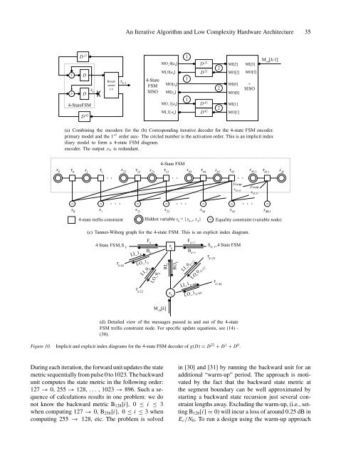
34 Yeung and ChuggIterative DecoderChannelInput z kADCChannelMetricRAM(1024x4x2)StateMetricRAM(512x9)BWD State Metric Recursion+ LI_0, LI_1, RI UpdateRIRAM(512x5x2)LI_0RAM(512x5x2)LI_1RAM(512x5x2)VerificationUnitAcquisitionDecisionFWD State Metric RecursionFigure 9. Block diagram of the acquisition module for g(D) = D 22 + D 1 + D 0 .4.1. 4-State FSM DecoderAs shown in Fig. 9, instead of using Fig. 7 as ourPN estimator architecture which has three 2-state FSMSISOs (one for g(D) = D 22 + D 1 + D 0 and two forg(D) = D 44 + D 2 + D 0 ), we combine the two modelstogether using a single 4-state FSM as shown in Fig.10(a). The new FSM captures all the information of theoriginal FSMs and lowers the memory requirementsfrom 4M messages plus state metrics to approximately3M messages plus state metrics as demonstrated below.Moreover, by using a single FSM, we save routing resourcesby lowering the bandwidth requirement for thechannel metrics (M ch [k] = z k ) memory since it is nowaccessed only by one FSM-SISO instead of three FSMSISOs. Using the 4-state FSM does require more logicin the FSM SISO implementation, but this increase isjustified by the the additional savings in memory androuting.Our 4-state FSM decoder is also based on the forwardbackward algorithm. We define the state as S k ={x k−1 , x k } and the corresponding decoder is shown inFig. 10(b). Again, this is an implicit index digram. Theexplicit index diagram (i.e., the Tanner-Wiberg graph)is shown in Fig. 10(c). The state transition table isshown in Table 1 and the messages passed are shownin detail in Fig. 10(d).The update equations are obtained by applying thestandard message passing rules [21] on either Fig. 10(b)or Fig. 10(c). They are listed from (14) to (30) in theappendix.Simulation results shows that the 4-state FSM decoderimplementation improves the performance by0.2 dB in E cN 0as compared to the three 2-state FSMimplementation.We can continue to combine multiple auxiliary modelsto form a single FSM. For example, we can implementa 3rd order model using a 16-state FSM. However,the exponential growth in state metric memorymay outweigh any savings in the message memory forlarger n.4.2. Forward Backward Algorithm Architecture forMultiple Index SegmentsTo reduce the internal FSM state metric memory, wedivide the observation window into multiple segmentsand run the forward backward algorithm (FBA) segmentby segment. This is a standard approach for implementingthe Viterbi and turbo decoders [30, 31].In our prototype system, we divide the observationwindow (1024) into 8 segments. There is one forwardunit and one backward unit running 15 iterations.Table 1.State transition table of the 4-state FSM.S k−1 = {x k−2 , x k−1 } S k = {x k−1 , x k } x k x k−22 x k−4400 (0) 00 (0) 0 0 000 (0) 01 (1) 1 1 101 (1) 10 (2) 0 1 001 (1) 11 (3) 1 0 110 (2) 00 (0) 0 0 110 (2) 01 (1) 1 1 011 (3) 10 (2) 0 1 111 (3) 11 (3) 1 0 0
An Iterative Algorithm and Low Complexity Hardware Architecture 35D 21MO_0[a k]1D -21 2MI[2]MI[3]M ch[k-1]+ D+ D4-StateFSMD 42x kBroadcaster(=)x k-14-StateFSMSISOMI_0[a k] D 21MO[x k]MI[x k]MO_1[a k]MI_1[ a k]11D -42D 4222MO[2]MI[0]MO[0]MI[1]MO[1]MO[3]=SISO(a) Combining the encoders for the (b) Corresponding iterative decoder for the 4-state FSM encoder.primary model and the 1 st order auxiliarymodel to form a 4-state FSM diagram.The circled number is the activation order. This is an implicit indexencoder. The output x k is redundant.s 04-State FSMτ s τ τ τ0112223τ τ τ44s M-1 M-145x M-45s M=x 0==x 1x 22s 22s 23=x 23=x 44s 44s 45=FromFromx M-23x 45=x M-14-state trellis constraint Hidden variable s k= {x k-1, x k} = Equality constraint (variable node)(c) Tanner-Wiberg graph for the 4-state FSM. This is an explicit index diagram.F k+14 State FSM, S k τS k+1, 4 State FSMB kτk-44LI_1 kτF kLO_1 kk-22LI_0 kLO_0 kRI kRO kx kkB k+1LI_0 k+22LI_1 k+44LO_0 k+22LO_1 k+44τk+22τk+44M ch[k](d) Detailed view of the messages passed in and out of the 4-stateFSM trellis constraint node. For specific update equations, see (14) -(30).Figure 10. Implicit and explicit index diagrams for the 4-state FSM decoder of g(D) = D 22 + D 1 + D 0 .During each iteration, the forward unit updates the statemetric sequentially from pulse 0 to 1023. The backwardunit computes the state metric in the following order:127 → 0, 255 → 128, . . . , 1023 → 896. Such a sequenceof calculations results in one problem: we donot know the backward metric B 128 [i], 0 ≤ i ≤ 3when computing 127 → 0, B 256 [i], 0 ≤ i ≤ 3 whencomputing 255 → 128, etc. The problem is solvedin [30] and [31] by running the backward unit for anadditional “warm-up” period. The approach is motivatedby the fact that the backward state metric atthe segment boundary can be well approximated bystarting a backward state recursion just several constraintlengths away. Excluding the warm-up, (i.e., settingB 128 [i] = 0) will incur a loss of around 0.25 dB inE c /N 0 . To run a design using the warm-up approach
Page 1: Journal of VLSI Signal Processing 4
Page 5 and 6: An Iterative Algorithm and Low Comp
Page 7: An Iterative Algorithm and Low Comp
Page 12 and 13: 36 Yeung and ChuggIteration 0 Itera
Page 14 and 15: 38 Yeung and ChuggM chChannelMetric
Page 16 and 17: 40 Yeung and ChuggF 0 = 0 (14)B M =
Page 18: 42 Yeung and Chugghe was an Assista

An Iterative Algorithm and Low Complexity Hardware Architecture ...

Create successful ePaper yourself

Delete template?

Save as template?