An Iterative Algorithm and Low Complexity Hardware Architecture ...

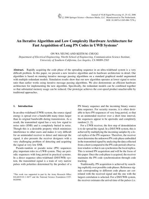
Journal of VLSI Signal Processing 43, 25–42, 2006c○ 2006 Springer Science + Business Media, LLC. Manufactured in The Netherlands.DOI: 10.1007/s11265-006-7278-yAn Iterative Algorithm and Low Complexity Hardware Architecture forFast Acquisition of Long PN Codes in UWB Systems ∗ON WA YEUNG AND KEITH M. CHUGGDepartment of Electrical Engineering, Viterbi School of Engineering, Communication Science Institute,University of Southern California, Los Angeles, CA 90089-2565Abstract. Rapidly acquiring the code phase of the spreading sequence in an ultra-wideband system is a verydifficult problem. In this paper, we present a new iterative algorithm and its hardware architecture in detail. Ouralgorithm is based on running iterative message passing algorithms on a standard graphical model augmentedwith multiple redundant models. Simulation results show that our new algorithm operates at lower signal to noiseratio than earlier works using iterative message passing algorithms. We also demonstrate an efficient hardwarearchitecture for implementing the new algorithm. Specifically, the redundant models can be combined togetherso that substantial memory usage can be reduced. Our prototype achieves the cost-speed product unachievable bytraditional approaches.1. IntroductionIn an ultra-wideband (UWB) system, the source signalenergy is spread over a bandwidth many times largerthan its original bandwidth during transmission. As aresult, the transmitted signal has a very low signal tonoise ratio (SNR) and is completely buried in noise.Though this is a desirable property which minimizesinterference to other users and makes it very difficultfor an unintended receiver to detect and intercept thesignal, it also presents the receiver designers with avery challenging problem of detecting and acquiringthe signal at very low SNR.Pseudo-random or pseudo noise (PN) sequencesplay important roles in a UWB system. They are periodicsequences with long period in practical systems.In a direct sequence ultra-wideband (DS/UWB) system,the transmitted signal is a train of very narrowpulses with polarities determined by the product of a∗ This work was supported in part by the Army Research OfficeDAAD19-01-1-0477 and the National Science Foundation CCF-0428940.PN binary sequence and the incoming binary sourcedata sequence. For security reasons, it is often desirableto have PN sequences of very long period, so thatto an unintended receiver over a short time interval,the sequences appear to be aperiodic and completelyrandom [1, 2].For a UWB receiver, the first step of demodulationis to de-spread the signal. In a DS/UWB system, this isachieved by multiplying the incoming samples by a localreplica of the PN sequence. Therefore, the receivermust determine the unknown PN code phase embeddedin the transmitted signal by analyzing the data collectedfrom a short (compared to the PN code period) observationwindow so that it can synchronize the local replica.This is termed PN acquisition and will be the focus ofthis paper. Once the code phase is acquired, the receivermaintains the PN code synchronization through codetracking.Traditionally, PN acquisition is achieved by searchingexplicitly over possible code phases. Reference signalscorresponding to different code phases are correlatedwith the received signal and the one with thelargest correlation is selected. For a DS/UWB system,the receiver estimates the arrival time of the pulses (i.e.

An Iterative Algorithm and Low Complexity Hardware Architecture 27g 0D+ ++ + +g 1g 2g r-3g r-2DD Dx k+r-1x k+r-2x k+3x k+2g r-1x k+1Dx kg rFigure 1.Linear feedback shift register (LFSR) structure for m-Sequence generation.ematically, the sequence structure can be expressedasx k = g 1 x k−1 ⊕ g 2 x k−2 ⊕ · · · ⊕ g r x k−r (1)where g 0 = g r = 1, g k ∈ {0, 1} for 1 < k < r and⊕ is the modulo-2 addition. The generator polynomialis g(D) = D r + g r−1 D r−1 + g r−2 D r−2 + · · · + D 0where D is the unit delay operator [10]. Given r,there is only a very limited set of g k values thatgenerates an m-Sequence. Because of their excellentcorrelation properties, m-Sequences are widely usedas spreading sequences in spread spectrum systems[1, 10].2.2. Signal ModelFor a DS/UWB system, a standard model for acquisitioncharacterization is [1, 2]z k = √ E c (−1) x k+ n k (2)where z k , 0 ≤ k ≤ M − 1, is the noisy sample receivedby the acquisition module, x k , 0 ≤ k ≤ M − 1, is thespreading m-Sequence, E c is the transmitted energy perpulse and n k is additive white Gaussian noise (AWGN)with variance N 02 . We also assume that x k is generatedby an r-stage LFSR and r ≪ M ≪ 2 r − 1. This isa much simplified model which does not include theeffect of jamming, oversampling, etc, but it is widelyused in literatures to benchmark the performance of PNacquisition algorithms. 1The goal of the acquisition module is to estimatex k based on z k 0 ≤ k ≤ M − 1 for a given frameepoch estimate and decide whether the frame epochestimate is correct. In our design, we obtain the estimateof x k , denoted by ˆx k , by running an iterative messagepassing algorithm. Because ˆx k has to be consistent with(1), once r consecutive ˆx k are obtained, the rest of thesequence is determined by extrapolating the estimateby (1). As the last step, z k is correlated with ˆx k , 0 ≤k ≤ M − 1 to check whether the correlation thresholdis reached.2.3. Iterative Message Passing Algorithm (iMPA)for Fast PN AcquisitionIn traditional PN acquisition approaches, the receivedsequence z k is correlated with up to 2 r − 1 PN sequencesgenerated by different x 0 , x 1 , . . . , x r−1 combinationsfor the whole observation window and thealgorithm chooses the phase corresponding to the highestcorrelation. In terms of computation complexity,the main difference between parallel search andserial/hybrid search is whether all correlations arecompleted every observation window. Since each correlationrequires M − 1 additions, the computationcomplexity is of O(M · 2 r ) for all of these traditionalapproaches. For parallel search, all valid configurationsof x k are correlated, we can therefore interpretit as maximum likelihood (ML) decoding ofx k from (2) and serial/hybrid search as approximationsto ML decoding. Based on this observation, weformulate the PN acquisition problem as a decodingproblem and apply an iterative message passing algorithmsimilar to turbo code [11, 12] or LDPC decoding[13–15].Since the inception of turbo codes, iterative messagepassing algorithms have been widely studied. Theycan be easily derived by constructing the correspondinggraphical models for the system and applying astandard set of rules. It is now understood that if thegraphical model has no cycles, the algorithm is equivalentto maximum likelihood decoding. Otherwise, the

An Iterative Algorithm and Low Complexity Hardware Architecture 29P 0[22] P 0[23] P 0[44] P 0[45] P 0[M-2] P 0[M-1]++ + + + += = = = = = = = = = =X[2]X[0]X[21] X[22] X[23] X[43] X[44] X[45] X[M-2] X[M-1]X[1]+ + + +P 1[44] P 1[45] P 1[M-2] P 1[M-1]Figure 3. Forming the 2nd order graphical model using the primary model (g(D) = D 22 + D 1 + D 0 ) and the 1st order auxiliary model(g(D) = D 44 + D 2 + D 0 ).This motivates us to find a better graphical model onwhich we can apply the standard iterative messagepassing algorithm and is more amenable to hardwareimplementation.extended to show thatg(D) = D 22·2n + D 2n + D 0 , n = 0, 1, 2, 3 . . . (6)2.4. Graphical Models with RedundancyTo improve the performance of the iMPA, we introducea new decoding graph for g(D) = D 22 + D 1 + D 0 . Itis constructed using multiple graphical models eachof which fully captures the PN code structure. In thissense, the model has redundancy. This is equivalent toadding redundant parity checks to the standard paritycheck matrix. The technique is also applied in soft decodingof some of the classical codes [26–28]. Fig. 3shows the special case of using two models. Each ofthe subgraphs is based on a different generator polynomialto the same m-Sequence. Mathematically, weintroduce reducible polynomials to generate the samesequence. For example, let x k be the sequence generatedby g(D) = D 22 + D 1 + D 0 , we have the followingequations:x k ⊕ x k−1 ⊕ x k−22 = 0 (3)x k−1 ⊕ x k−2 ⊕ x k−23 = 0 (4)x k−22 ⊕ x k−23 ⊕ x k−44 = 0 (5)Adding (3), (4) and (5) together, we have x k +x k−2 +x k−44 = 0. Therefore, g(D) = D 44 +D 2 +D 0 also generatesthe same sequence. The argument can be easilyall generate the same sequence. In this paper, we referthe graphical model based on (6) as the nth order auxiliarymodel and the one based on g(D) = D 22 +D 1 +D 0as the primary model. Also, we refer to the modelthat combines the primary model and the 1st, 2nd. . . (n − 1)th order auxiliary models as the nth ordermodel. Our decoding graph for an nth order model isformed by constraining the output of primary modeland each of the ith order auxiliary model 1 ≤ i ≤ nto be equal. As an example, the graph of the 2nd ordermodel is shown in Fig. 3. The performance improvementby combining multiple models is shown in Fig. 4.Even though each individual auxiliary model producesvery unreliable decoding decisions, combining themimproves the convergence behaviour dramatically. Wegain around 1 dB gain for each additional auxiliarymodel introduced. Only 10 iterations are required forpractical convergence for a 5th order model. Our multiplemodel algorithm also works for other m-Sequences.As a comparison, Fig. 5 shows the performance forg(D) = D 15 + D 1 + D 0 where the curve for algorithmin [2] is also included.Our baseline algorithm is summarized in Algorithm1. The complexity of both the decoding andcorrelation operations is of O(M), therefore our algorithmis also of O(M) complexity. There is substantialcomplexity reduction compared to the traditional

30 Yeung and ChuggAlgorithm 1: Baseline iMPA algorithm for fast PN acquisition.approaches. Also, our new algorithm offers better performancewith no additional complexity compared tothe approach in [2] since we reduce the number of iterationsdramatically.3. Hardware Architecture for Iterative DecoderIn this section, we present the hardware architectureof the basic building blocks in our iMPA algorithm.Assuming using an nth order model, the pulses are decodedby n different models during each iteration. Thehardware module that performs the iterative messagepassing algorithm for each auxiliary model is an iterativedecoder.3.1. Forward Backward Algorithm Based IterativeDecoderThe basic building block in our algorithm is an iterativedecoder that decodes the sequence generated byg(D) = D 22 + D 1 + D 0 . We have two hardware architecturecandidates: one based on Fig. 2(a) and anotherbased on Fig. 2(b). Simulation shows that both architecturesperforms similarly (the difference in sensitivity isless than 0.3 dB).If we choose the Tanner graph representation asshown in Fig. 2(a), the number of messages neededto be saved in each iteration equals to the number ofedges in the graph. Therefore, the minimum storagerequirement is 3M messages.Alternatively, if we base our decoder on a Tanner-Wiberg graph [16] with hidden variables introduced asshown in Fig. 2(b), we have a more memory efficienthardware architecture. Equations similar to [2, (23)]to [2, (29)] can readily be obtained from this graph.This graph is an explicit index diagram [21, 25]. Forreaders not familiar with Tanner-Wiberg graph, the updateequations may be more easily explained by consideringFig. 6(a) which decomposes the sequence generatingLFSR structure into three parts: one 2-stateg(D) = D + 1 finite state machine (FSM) 2 , one delayblock (D 21 ) and one broadcaster (i.e., an equalityconstraint). Applying the standard iterative messagepassing rules [21, 25], we derive the decodinggraph (Fig. 6(b)) by replacing each component by asoft-in soft-out (SISO) module which performs the a-posteriori probability (APP) decoding [29].

An Iterative Algorithm and Low Complexity Hardware Architecture 310.98P acqversus E c/N 0, M=1024, g(D)=D 22 +D 1 +D 00.960.94(6,15)(5,10)P acq0.920.9(5,20)(5,15)(3,15)(2,15)0.880.86(4,15)(1,15)(2,15), Hardwarearchitecture(n,I): n = model orderI = # iterations-14 -13 -12 -11 -10 -9 -8 -7E c/N 0(dB)Figure 4. Acquisition performance vs. E c /N 0 for using an nth order model on g(D) = D 22 + D 1 + D 0 . The acquisition performance of ourhardware implementation (see Section 4) is marked as “(2,15), hardware architecture”.0.980.960.94(6,15)P acq0.92(5,15)(4,15)0.9(3,15)[2],100 iter.(2,15)(1,15)0.880.86(n,I):n = model orderI = # iterations-15 -14 -13 -12 -11 -10 -9 -8E c/N 0(dB)Figure 5. Acquisition performance vs. E c /N 0 for using an nth order model on g(D) = D 15 + D 1 + D 0 . As a reference, the acquisitionperformance by running the [2] algorithm is marked as “ [2], 100 iter.”.

An Iterative Algorithm and Low Complexity Hardware Architecture 33g(D)=D 22 +D 1 +D 0Modelg(D)=D 44 +D 2 +D 0Model=g(D)=D 22 +D 1 +D 0Decoderg(D)=D 44 +D 2 +D 0x k Decoder1212Broadcaster(=)SISOM ch [k]g(D)=D 22x2 n-1+D 2 n-1+D 0Modelg(D)=D 22x2 n-1+D 2 n-1+D 0Decoder12(a)(b)Figure 7. Iterative decoder architectures for an nth order model: (a) is the combined model; (b) is the iterative decoder architecture with theactivation order circled.D 21 x kx k-1MO[a_0 k]1D -21 2MI[2]MI[3]M ch[k-1]a_0 k+ Da_1 k+ D4-State FSMD 42Broadcaster(=)x k-14-StateFSMSISOMI[ a_0 k] D 21MO[x k-1]MI[ x k-1]MO[a_1 k]MI[ a_1 k]11D -42D 4222MO[2]MI[0]MO[0]MI[1]MO[1]MO[3]=SISO(a) Decomposition of a g(D) = D 44 +D 2 +D 0FSM into two g(D) = D 22 + D 1 + D 0 FSMsby index partitioning.(b) g(D) = D 44 + D 2 + D 0 decoder architecture.Figure 8.Implementing a g(D) = D 44 + D 2 + D 0 decoder using two g(D) = D 22 + D 1 + D 0 decoders.3.3. Simplification of an Auxiliary Model DecoderUsing Index PartitioningAn advantage of using auxiliary models defined as (6)is that all auxiliary decoders can be constructed usingthe g(D) = D 22 + D 1 + D 0 decoder. This is achievedby index partitioning on the output of the higher ordermodel. Specifically, the index partitioned output isequivalent to the output of the primary model.As an example, consider the FSM that generates theg(D) = D 44 + D 2 + D 0 sequence. As shown in Fig.8(a), we can model this as two identical FSMs eachgenerating the x k = x k−1 + x k−22 sequence. One generatesthe sequence at odd indices and the other generatesthe sequence at even indices. The correspondingdecoder is shown in Fig. 8(b) which consists of twog(D) = D 22 + D 1 + D 0 decoders. In this case, sinceeach decoder only decodes M/2 pulses, the total memoryrequirement for messages is the same as an M-pulseg(D) = D 22 + D 1 + D 0 decoder.This idea extends to higher order auxiliary modeldecoders. Specifically, x k generated by (6) can be partitionedinto 2 n sub-sequences: x 2 n k+i, 0 ≤ i ≤ 2 n − 1with each sub-sequence generated by g(D) = D 22 +D 1 + D 0 . The corresponding decoder can be constructedusing multiple g(D) = D 22 + D 1 + D 0 decoderssimilar to Fig. 8(b).4. Hardware ArchitectureIn this section, we consider the case of decoding the PNsequence g(D) = D 22 + D 1 + D 0 over an observationwindow of M = 1024 using the 2nd order model architecture.The block diagram of our acquisition moduleis shown in Fig. 9.

34 Yeung and ChuggIterative DecoderChannelInput z kADCChannelMetricRAM(1024x4x2)StateMetricRAM(512x9)BWD State Metric Recursion+ LI_0, LI_1, RI UpdateRIRAM(512x5x2)LI_0RAM(512x5x2)LI_1RAM(512x5x2)VerificationUnitAcquisitionDecisionFWD State Metric RecursionFigure 9. Block diagram of the acquisition module for g(D) = D 22 + D 1 + D 0 .4.1. 4-State FSM DecoderAs shown in Fig. 9, instead of using Fig. 7 as ourPN estimator architecture which has three 2-state FSMSISOs (one for g(D) = D 22 + D 1 + D 0 and two forg(D) = D 44 + D 2 + D 0 ), we combine the two modelstogether using a single 4-state FSM as shown in Fig.10(a). The new FSM captures all the information of theoriginal FSMs and lowers the memory requirementsfrom 4M messages plus state metrics to approximately3M messages plus state metrics as demonstrated below.Moreover, by using a single FSM, we save routing resourcesby lowering the bandwidth requirement for thechannel metrics (M ch [k] = z k ) memory since it is nowaccessed only by one FSM-SISO instead of three FSMSISOs. Using the 4-state FSM does require more logicin the FSM SISO implementation, but this increase isjustified by the the additional savings in memory androuting.Our 4-state FSM decoder is also based on the forwardbackward algorithm. We define the state as S k ={x k−1 , x k } and the corresponding decoder is shown inFig. 10(b). Again, this is an implicit index digram. Theexplicit index diagram (i.e., the Tanner-Wiberg graph)is shown in Fig. 10(c). The state transition table isshown in Table 1 and the messages passed are shownin detail in Fig. 10(d).The update equations are obtained by applying thestandard message passing rules [21] on either Fig. 10(b)or Fig. 10(c). They are listed from (14) to (30) in theappendix.Simulation results shows that the 4-state FSM decoderimplementation improves the performance by0.2 dB in E cN 0as compared to the three 2-state FSMimplementation.We can continue to combine multiple auxiliary modelsto form a single FSM. For example, we can implementa 3rd order model using a 16-state FSM. However,the exponential growth in state metric memorymay outweigh any savings in the message memory forlarger n.4.2. Forward Backward Algorithm Architecture forMultiple Index SegmentsTo reduce the internal FSM state metric memory, wedivide the observation window into multiple segmentsand run the forward backward algorithm (FBA) segmentby segment. This is a standard approach for implementingthe Viterbi and turbo decoders [30, 31].In our prototype system, we divide the observationwindow (1024) into 8 segments. There is one forwardunit and one backward unit running 15 iterations.Table 1.State transition table of the 4-state FSM.S k−1 = {x k−2 , x k−1 } S k = {x k−1 , x k } x k x k−22 x k−4400 (0) 00 (0) 0 0 000 (0) 01 (1) 1 1 101 (1) 10 (2) 0 1 001 (1) 11 (3) 1 0 110 (2) 00 (0) 0 0 110 (2) 01 (1) 1 1 011 (3) 10 (2) 0 1 111 (3) 11 (3) 1 0 0

An Iterative Algorithm and Low Complexity Hardware Architecture 35D 21MO_0[a k]1D -21 2MI[2]MI[3]M ch[k-1]+ D+ D4-StateFSMD 42x kBroadcaster(=)x k-14-StateFSMSISOMI_0[a k] D 21MO[x k]MI[x k]MO_1[a k]MI_1[ a k]11D -42D 4222MO[2]MI[0]MO[0]MI[1]MO[1]MO[3]=SISO(a) Combining the encoders for the (b) Corresponding iterative decoder for the 4-state FSM encoder.primary model and the 1 st order auxiliarymodel to form a 4-state FSM diagram.The circled number is the activation order. This is an implicit indexencoder. The output x k is redundant.s 04-State FSMτ s τ τ τ0112223τ τ τ44s M-1 M-145x M-45s M=x 0==x 1x 22s 22s 23=x 23=x 44s 44s 45=FromFromx M-23x 45=x M-14-state trellis constraint Hidden variable s k= {x k-1, x k} = Equality constraint (variable node)(c) Tanner-Wiberg graph for the 4-state FSM. This is an explicit index diagram.F k+14 State FSM, S k τS k+1, 4 State FSMB kτk-44LI_1 kτF kLO_1 kk-22LI_0 kLO_0 kRI kRO kx kkB k+1LI_0 k+22LI_1 k+44LO_0 k+22LO_1 k+44τk+22τk+44M ch[k](d) Detailed view of the messages passed in and out of the 4-stateFSM trellis constraint node. For specific update equations, see (14) -(30).Figure 10. Implicit and explicit index diagrams for the 4-state FSM decoder of g(D) = D 22 + D 1 + D 0 .During each iteration, the forward unit updates the statemetric sequentially from pulse 0 to 1023. The backwardunit computes the state metric in the following order:127 → 0, 255 → 128, . . . , 1023 → 896. Such a sequenceof calculations results in one problem: we donot know the backward metric B 128 [i], 0 ≤ i ≤ 3when computing 127 → 0, B 256 [i], 0 ≤ i ≤ 3 whencomputing 255 → 128, etc. The problem is solvedin [30] and [31] by running the backward unit for anadditional “warm-up” period. The approach is motivatedby the fact that the backward state metric atthe segment boundary can be well approximated bystarting a backward state recursion just several constraintlengths away. Excluding the warm-up, (i.e., settingB 128 [i] = 0) will incur a loss of around 0.25 dB inE c /N 0 . To run a design using the warm-up approach

36 Yeung and ChuggIteration 0 Iteration 111521024512Clock384256Bwd/ Upd Seg. 0Rd. F 127:0fromSMM[127:0]Rd. CMB0Wr. MBB0Fwd Seg. 0Wr. F 0:127toSMM[0:127]Rd. CMB0Rd. MBB0Stores B 128Bwd/ Upd Seg. 0Rd. F 127:0fromSMM[127:0]Rd. CMB0Wr. MBB0Bwd/Upd Seg. 1Rd. F 255:128fromSMM[0:127]Rd. CMB1Wr. MBB1Fwd Seg. 1Wr. F 128:255toSMM[127:0]Rd. CMB1Rd. MBB1Copies B 128from Iteration 0StoresB 256Bwd/Upd Seg. 1Rd. F 255:128fromSMM[0:127]Rd. CMB1Wr. MBB1Copies B 256from Iteration 0Fwd Seg. 2Wr. F 256:383to SMM[0:127]Rd. CMB0Rd. MBB0Bwd/Upd Seg. 2Rd. F 383:256fromSMM[127:0]Rd. CMB0Wr. MBB0Fwd Seg. 2Wr. F 256:383to SMM[0:127]Rd. CMB0Rd. MBB0Summary of Abbreviations:Fwd.: ForwardBwd: BackwardUpd: UpdateSeg.: SegmentWr.: WriteRd.: ReadF i:j: Forward State Metric F k, k=i to jB i:j: Backward State Metric B k,k= i to jSMM: State Metric MemoryCMB0: Channel Metric Bank 0CMB1: Channel Metric Bank 1MBB0: Message Buffer Bank 0MBB1: Message Buffer Bank 1There are 3 messages buffers: RI, LI_0and LI_11280Fwd Seg. 1Wr. F 128:255to SMM[127:0]Rd. CMB1Rd. MBB1Fwd Seg. 0Wr. F 0:127to SMM[0:127]Rd. CMB0Rd. MBB0128 256 384 512Channel Observation Index (k)Figure 11.Processing and memory access pipeline for the 4-state decoder.at full-speed, an additional backward unit is requiredso that one unit warms up while the other is doing theupdate [30, 31]. The additional unit can be saved ifwe do not use the warm-up approach but instead copythe B 128 [i] values from the previous iteration. This isfeasible because the warm-up period is only requiredif we are trying to approximate an FBA-SISO in isolation.For an iterative system, starting the backward

An Iterative Algorithm and Low Complexity Hardware Architecture 370.980.96(4,5)0.94Floating Point(5,16)(4,4)P acq0.92(4,16)(4,16) Mid-pt.Loading(3,16)0.9(4,6)0.880.86(#Bit ADC, #Bit Metric)-10 -9.8 -9.6 -9.4 -9.2 -9 -8.8 -8.6E c/N 0(dB)Figure 12. P acq vs. E c /N 0 for different bit width combinations, g(D) = D 22 + D 1 + D 0 .iteration based on earlier iteration value is equivalent toa change in the activation schedule for the iMPA on thecyclic graph, and as such does not significantly affectthe performance. This is a known architecture for implementingiterative decoders with forward-backwardbased SISO decoders (e.g., see [32–34]). Once both theforward and backward state metrics become available,LI 0 k , LI 1 k , RI k and M dec [k] are computed and theFSM state metric memory is released immediately. Theprocessing pipeline is shown in Fig. 11 which shows theupdate sequence as well as the corresponding memoryaccess.4.3. Bit WidthThe bit widths in our system are determined by simulationsin two steps. First, we fixed LI 0 k , LI 1 k , RI k tobe of 16 bits and determine that 4 bits of ADC outputis sufficient. Compared to floating point, there is onlya performance loss of 0.2 dB.The performance for various bit width combinationsis shown in Fig. 12. For each ADC bit width, we haveoptimized the scale q that sets the ADC dynamic range(ADC out = quantize(q · z k )) for performance. For a4-bit ADC, q opt is found to be 1.65 by simulation. As areference, we also show the performance for the standardmid-point loading q = 3.5 when the ADC is of4 bits.The second step is to determine the bit width for themessages LI 0, LI 1 and RI. This is necessary sincetheir values may grow as the decoder iterates. To avoidusing excessive bits for storage, we have to clip themafter each (FBA/=) SISO activation. As shown in Fig.12, 5 bits are sufficient for our application when theADC bit width is 4.To determine the bit width for the state metric, werely on the fact that for a given k, we are only interestedin the difference between F k [i] 0 ≤ i ≤ 3, nottheir values. Therefore, we only need the bit width tobe big enough for the differences. If we subtract F k [0]from F k [i] 0 ≤ i ≤ 3, the differences (i.e., the normalizedF k [i]) can be shown to be bounded between −128to 127 for 5-bit messages by an argument similar to theones in [35] and [21]. As a result, it can be representedby 8 bits. Similarly, the normalized B k [i] 0 ≤ i ≤ 3can be represented by 8 bits for 0 ≤ k ≤ 1024. Also,we do not need to store the normalized F k [0] and B k [0]since they are always 0. The normalization approach iswhat we apply for all binary variables because it savesthe memory usage by half and only requires one subtraction.For example, LI 0 k is a shorthand for LI 0 k [1]

38 Yeung and ChuggM chChannelMetricAccessUnit+Σ+Correlator0MUX1DThresholdAcquisitionDecision-Σ+PN_ESTIMATEPNExtrapolationFigure 13.Verification unit for the PN acquisition module.where LI 0 k [0] = 0 ∀ k. For the 4-ary state metric variablesF k [i] and B k [i], the normalization approach is lessattractive. It only reduces the memory usage by onefourthat the expense of impacting the frequency scalingof our circuit by requiring three additional subtractionsin the critical path of the forward and backward recursions.As a result, we do not perform normalizationand use 9 bits to represent the state metric instead of 8bits. This additional 1-bit approach is commonly usedin Viterbi decoders and is proven to be correct in [35]under the condition that two’s complement arithmeticis used.4.4. Partitioning the Memory into BanksIn our prototype design, we have several modules concurrentlyaccessing memory. By carefully partitioningthe memory, contention can be avoided without the useof multiport memory. The access pipeline for the abovememories is shown in Fig. 11.For the message memories (LI 0, LI 1 and RI), wedivide them into two banks of 512 entries. One bankis for the odd FBA segment and the other for the evenFBA segment. By this arrangement, there are at most 2concurrent accesses and we can implement LI 0, LI 1and RI using 2-port memories.For the FSM state metric, the forward unit writesto the memory while both the backward and LI 0,LI 1 RI update unit read the same data from the memory.As a result, we only need a single bank of 2-portmemories.The channel metric memory is divided into twobanks each comprising 1024 entries. The ADC and theacquisition module always work on different banks.By subdividing each bank into two sub-banks, one forthe FBA odd segment and the other for the FBA evensegment, there are at most two simultaneous accessesto the same segment. Therefore, the channel metriccan also be implemented by 2-port memories. In orderto reuse the state metric memory once the backwardmetric is computed, the FSM state metric are storedin the physical memory in reverse order for even segments.For example, the even segment F 128 to F 255 arestored in the state metric memory [127:0] while theodd segment F 0 to F 127 are stored in the state metricmemory [0:127]. The details are also shown inFig. 11.For design simplicity, we used 2-port memories inour prototype implementation since it is free in ourtarget device (Xilinx Virtex II FPGA). However, thedesign can be easily ported to single port memory onlyarchitecture by doubling the bus width and time divisionmultiplexing the access.4.5. Verification UnitOur verification unit, shown in Fig. 13, consists of twoparts, a PN sequence extrapolation unit and a correlatorunit. The extrapolation unit extends the 22-bit PNestimate it receives to the whole observation window.The correlation unit then correlates this sequence withthe channel metric. To improve efficiency, the correlatoroutput is checked every M pulses and it must4exceed the check point threshold before continuing. Ifthe final correlation value exceeds the final threshold,acquisition is declared. The final threshold is chosento be 0.65 · q · 1024 found by simulation so that thefrequency of false alarm is 0 in 5000 trials when signal

An Iterative Algorithm and Low Complexity Hardware Architecture 39is absent while minimizing the probability of rejectingthe correct estimate when signal is present.4.6. Hardware ImplementationWe implemented the architecture using Verilog HDL.The code is synthesized by Synplicity, then mappedby Xilinx Foundation to a Xilinx Virtex 2 device(XC2v250-6). The number of bits implemented inblock RAM is 28160, the number of 4-input LUTsused is 2433 and the number of slices used is 1481.The design can run at 91 MHz. These figures show thatmemory is the main component of the circuit and justifyour decision to trade off logic for memory reduction.Our baseline design can decode Freq clkpulses per15second. Assuming a 60 MHz clock, our prototype generatesa PN code phase decision every1560 MHz · 1024 =2.56 µs. The decode process has to be repeated for eachframe epoch estimate until the correct frame epoch isfound. Assuming the frame time T f = 250 ns (i.e.pulse rate = 4 Mpulses/s) and pulse width T p = 1.6 ns,the approximate average acquisition time of our prototypesystem T acq = 2.56 µs · T fT p· 0.5 = 20 ms withP acq = 0.95 at E cN 0= −8.9 dB. This assumes that halfof the frame epoch values are searched on average. Underthese noise level conditions with no signal present,5000 blocks were processed and acquisition was neverdeclared.As a comparison, to achieve the same average T acq ,hardware based on parallel search and running at thesame frequency requires approximately 5.6 × 10 5 correlators,5.6 × 10 5 14-bit comparators and 5.6 × 10 54-bit registers. For serial search, the hardware is trivialif we assume a one addition per clock architecture.However, it takes an average of 5.6 × 10 3 s (approximately1.5 hours) to acquire the PN sequence if runningat the same frequency.To further lower T acq , we can use parallel FBA architectures(i.e., instantiating multiple forward and backwardunits to process multiple data segments in parallel).We expect that the increase in logic will beapproximately linear when the speed up factor doesnot exceed 8 because we already divide the observationwindow into 8 segments in our iterative decoderand each of them can be run in parallel. For lowerspeed applications, our design can be further simplifiedto using single port memory and running the updatesequentially. Such a design can save in the numberof adders and reduce the routing resources. Thereforewe expect the logic gate count will scale linearlyfor target pulse rate varies from 500 kpulses/s to 32Mpulses/s.Our design can also be directly extended to operate ateven lower SNR. This requires adding auxiliary modeldecoders as well as memories for saving the messagesfrom the additional decoders. Since a 6th order modelis approximately three times more complex than a 2ndorder model, we estimate that the operating E c /N 0 canbe lowered to −13 dB by tripling the gate count oralternatively, increasing the acquisition time by 3 timesand tripling the message memory.5. ConclusionIn this paper, we present a new hardware architecturefor fast PN acquisition in UWB systems based on iterativemessage passing on a graphical model with redundancies.Our new algorithm improves sensitivity significantlyvia the introduction of multiple redundant models.Hardware based on the algorithm is economical toimplement and can rapidly acquire very long PN sequences,There is no known way to accomplish with traditionalapproaches using similar hardware resources.We examined in detail the design trade-offs in choosingan appropriate architecture for the main component:a forward backward algorithm based decoder. We thendemonstrated how to combine multiple redundant modelsinto a single model to reduce memory usage. Finally,we gave a detailed account on our hardware implementationand discuss various implementation techniques.Our design can be fit to a small FPGA while full parallelsearch is impractical to implement and serial searchis fiver orders of magnitude slower than our design.Future work will be focused on designing hardwarefor a more complicated system model which will incorporatesoversampling, interference and multi-pathchannel distortions.Appendix: Update Equations for the 4 State FSMDecoderThe update equations for the FSM are direct applicationof the standard message passing algorithms [21] on Fig.10(c). The variables F k , B k , LI 0 k , LI 1 k and RI k aredefined in Fig. 10(d). Alternatively, they can be derivedfrom Fig. 10(b) by applying standard SISO update rulesto each SISO. We list the equations based on Fig. 10(c)because it is easier to compare against [2, (23)]–[2, (29)].

40 Yeung and ChuggF 0 = 0 (14)B M = 0 (15)F k+1 [0] = min(F k [0], F k [2] + LI 1 k ) (16)F k+1 [1] = min(F k [0] + RI k + LI 0 k + LI 1 k ,F k [2] + RI k + LI 0 k ) (17)F k+1 [2] = min(F k [1] + LI 0 k , F k [3] + LI 0 k+LI 1 k ) (18)F k+1 [3] = min(F k [1] + RI k + LI 1 k , F k [3] + RI k )(19)B k−1 [0] = min(B k [0], B k [1] + RI k + LI 0 k+LI 1 k ) (20)B k−1 [1] = min(B k [2] + LI 0 k , B k [3] + RI k + LI 1 k )(21)B k−1 [2] = min(B k [0] + LI 1 k , B k [1] + RI k + LI 0 k )(22)B k−1 [3] = min(B k [2] + LI 0 k + LI 1 k , B k [3] + RI k )(23)RI k = LO 0 k+22 + LO 1 k+44 + M ch [k] (27)LI 0 k+22 = RO k + LO 1 k+44 + M ch [k] (28)LI 1 k+44 = RO k + LO 0 k+22 + M ch [k] (29)M dec = RO k + LO 0 k+22 + LO 1 k+44 + M ch [k]Acknowledgment(30)The authors would like to thank Mingrui Zhu for helpfuldiscussion on this research.Notes1. As shown in [2], this model and the algorithms developed inthis paper can be modified to work in sinusoidal carrier systemssuch as direct sequence spread spectrum system (DS/SS). In suchsystems, the model of (2) should be generalized to account for anunknown carrier phase, θ c . The approach suggested in [2] is tosearch over a finite set of carrier phase values.2. Note that this is the feedback polynomial. Viewed as a code, thegenerator is 1/(1 + D), which is an accumulator.ReferencesLO 0 k = min(F k [0] + B k+1 [1] + RI k + LI 1 k , F k [1]+ B k+1 [2], F k [2] + B k+1 [1] + RI k , F k [3]+ B k+1 [2] + LI 1 k ) − min(F k [0] + B k+1 [0],(24)F k [1] + B k+1 [3] + RI k + LI 1 k , F k [2]+B k+1 [0] + LI 1 k , F k [3] + B k+1 [3] + RI k )LO 1 k = min(F k [0] + B k+1 [1] + RI k + LI 0 k , F k [1]+B k+1 [3] + RI k , F k [2] + B k+1 [0], F k [3]+B k+1 [2] + LI 0 k ) − min(F k [0] + B k+1 [0],(25)F k [1] + B k+1 [2] + LI 0 k , F k [2] + B k+1 [1]+RI k + LI 0 k , F k [3] + B k+1 [3] + RI k )RO k = min(F k [0] + B k+1 [1] + LI 0 k + LI 1 k ,F k [1] + B k+1 [3] + LI 1 k , F k [2] + B k+1 [1]+LI 0 k , F k [3] + B k+1 [3]) − min(F k [0]+B k+1 [0], F k [1] + B k+1 [2] + LI 0 k , (26)F k [2] + B k+1 [0] + LI 1 k , F k [3] + B k+1 [2]+LI 0 k + LI 1 k )1. M.K. Simon, J.K. Omura, R.A. Scholtz, and B.K. Levitt, SpreadSpectrum Communications Handbook, McGraw-Hill, 1994.2. K.M. Chugg and M. Zhu, “A New Approach to Rapid PN CodeAcquisition using Interative Message Passing Techniques,”IEEE J. Select. Areas Commun., vol. 23, no. 51, June 2005.3. E.A. Homier and R.A. Scholtz, “Rapid Acquisition of Ultra-Wideband Signals in the Dense Multipath Channel,” in Digestof Papers, IEEE Conference on Ultra Wideband Systems andTechnologies, May 2002, pp. 105–109.4. M. Zhu and K.M. Chugg, “Iterative Message Passing Techniquesfor Rapid PN code Acquisition,” in Proc. IEEE MilitaryComm. Conf., Boston, MA, October 2003, pp. 434–439.5. I.D. O’Donnell, S.W. Chen, B.T. Wang, and R.W. Brodersen,“An Integrated, Low Power, Ultra-Wideband ReansceriverArchitecture for Low-Rate, Indoor Wireless Systems,” IEEECAS Workshop on Wireless Communications and Networking,September 2002.6. A. Polydoros and C.L. Weber, “A Unified Approach to SerialSearch Spread-Spectrum Code Acquisition,” IEEE Trans. Commununication,vol. 32, pp. 542–560, 1984.7. L. Yang and L. Hanzo, “Iterative Soft Sequential EstimationAssisted Acquisition of m-Sequence,” IEE Electronics Letters,vol. 38, no. 24, 2002, pp. 1550–1551.8. R.G. Gallager, “Acquisition of I-Sequences Using RecursiveSoft Sequential estimation,” IEEE Trans. Commununication,vol. 52, no. 2, Feb 2004 pp. 199–204.9. B. Vigoda, J. Dauwels, N. Gershenfeld, and H. Loeliger, “Low-Complexity lfsr Synchronization by Forward-only MessagePassing,” IEEE Trans. Information Theory, June 2003, submitted.

An Iterative Algorithm and Low Complexity Hardware Architecture 4110. S.W. Golomb, Shift Register Sequences, revised edition. AegeanPark Press, 1982.11. C. Berrou, A. Glavieux, and P. Thitmajshima, “Near ShannonLimit Error-Correcting Coding and Decoding: Turbo-Codes,”in Proc. International Conf. Communications, Geneva, Switzerland,pp. 1064–1070, 1993.12. C. Berrou and A. Glavieux, “Near Optimum Error CorrectingCoding and Decoding: Turbo-Codes,” IEEE Trans. Commununication,vol. 44, no. 10, pp. 1261–1271, October 1996.13. R.G. Gallager, “Low Density Parity Check Codes,”IEEE Trans. Information Theory, vol. 8, January 1962pp. 21–28.14. R.G. Gallager, Low-Density Parity-Check Codes. MIT Press,Cambridge, MA, 1963.15. D.J.C. MacKay and R.M. Neal, “Near Shannon Limit Performanceof Low Density Parity Check Codes,” IEE ElectronicsLetters, vol. 32, no. 18, August 1996 pp. 1645–1646.16. N. Wiberg, Codes and Decoding on General Graphs, Ph.D. dissertation,Linköping University (Sweden), 1996.17. R.J. McEliece, D.J.C. MacKay, and J.F. Cheng, “Turbo Decodingas an Instance of Pearl’s “Belief Propagation” Algorithm,”IEEE J. Select. Areas Commun., vol. 16, February 1998, pp.140–152.18. S.M. Aji, “Graphical Models and Iterative Decoding,” Ph.D.dissertation, California Institute of Technology, 1999.19. S.M. Aji and R.J. McEliece, “The Generalized DistributiveLaw,” IEEE Trans. Information Theory, vol. 46, no. 2, pp. 325–343, March 2000.20. F. Kschischang, B. Frey, and H.-A. Loeliger, “Factor Graphs andthe Sum-Product Algorithm,” IEEE Trans. Information Theory,vol. 47, Feb. 2001, pp. 498–519.21. K.M. Chugg, A. Anastasopoulos, and X. Chen, Iterative Detection:Adaptivity, Complexity Reduction, and Applications.Kluwer Academic Publishers, 2001.22. S. Benedetto and G. Montorsi, “Design of Parallel ConcatenatedConvolutional Codes,” IEEE Trans. Commununication, vol. 44,May 1996, pp. 591–600.23. S. Benedetto, D. Divsalar, G. Montorsi, and F. Pollara, “SerialConcatenation of Interleaved Codes: Performance Analysis, Design,and Iterative Decoding,” IEEE Trans. Information Theory,vol. 44, no. 3, May 1998, pp. 909–926.24. R.M. Tanner, “A Recursive Approach to Low ComplexityCodes,” IEEE Trans. Information Theory, vol. IT-27, September,pp. 533–547, 1981.25. S. Benedetto, D. Divsalar, G. Montorsi, and F. Pollara, “Soft-Input Soft-Output Modules for the Construction and DistributedIterative Decoding of Code Networks,” EuropeanTrans. Telecommun., vol. 9, no. 2, March/April, pp. 155–172,1998.26. J.S. Yedidia, J. Chen, and M. Fossorier, “Generating Code RepresentationsSuitable for Belief Propagation Decoding,” in Proc.40-th Allerton Conference Commun., Control, and Computing,Monticello, IL., October 2002.27. N. Santhi and A. Vardy, “On the Effect of Parity-Check Weightsin Iterative Decoding,” in Proc. IEEE Internat. Symp. InformationTheory, Chicago, IL., July 2004, p. 322.28. M. Schwartz and A. Vardy, “On the Stopping Distance and theStopping Redundancy of Codes,” IEEE Trans. Information Theory,2005, submitted.29. L.R. Bahl, J. Cocke, F. Jelinek, and J. Raviv, “Optimal Decodingof Linear Codes for Minimizing Symbol Error Rate,” IEEETrans. Information Theory, vol. IT-20, 1974, pp. 284–287.30. A.J. Viterbi, “Justification and Implementation of the MAP Decoderfor Convolutional Codes,” IEEE J. Select. Areas Commun.,vol. 16, February 1998, pp. 260–264.31. G. Masera, G. Piccinini, M.R. Roch, and M. Zamboni, “VLSIArchitectures for Turbo Codes,” IEEE Trans. VLSI, vol. 7, no. 3,1999.32. J. Dielissen and J. Huisken, “State Vector Reduction for Initializationof Sliding Windows MAP,” in 2nd Internation Symposiumon Turbo Codes & Related Topics, Brest, France, 2000, pp.387–390.33. S. Yoon and Y. Bar-Ness, “A Parallel MAP Algorithm forLow Latency Turbo Decoding,” IEEE Communications Letters,vol. 6, no. 7, 2002, pp. 288–290.34. A. Abbasfar and K. Yao, “An Efficient and Practical Architecturefor High Speed Turbo Decoders,” in IEEE 58th VehicularTechnology Conference, Vol. 1, 2003, pp. 337–341.35. A.P. Hekstra, “An Alternative to Metric Rescaling in Viterbi Decoders,”IEEE Trans. Commununication, vol. 37, no. 11, November1989.On Wa Yeung received the B. Eng. degree in Electronic Engineeringfrom the Chinese University of Hong Kong, Hong Kong in 1994 andMSEE from the University of Southern California (USC) in 1996. In1997–2003, he was a hardware engineer in Hughes Network Systems,San Diego, CA, designing hardware platforms for fixed wireless andsatellite terminals. He is currently working towards the Ph.D. degreein EE at USC. His research interests are in the areas of iterativedetection algorithms and their hardware implementation.oyeung@usc.eduKeith M. Chugg (S’88-M’95) received the B.S. degree (high distinction)in Engineering from Harvey Mudd College, Claremont, CA in1989 and the M.S. and Ph.D. degrees in Electrical Engineering (EE)from the University of Southern California (USC), Los Angeles, CAin 1990 and 1995, respectively. During the 1995–1996 academic year

42 Yeung and Chugghe was an Assistant Professor with the Electrical and Computer EngineeringDept., The University of Arizona, Tucson, AZ. In 1996 hejoined the EE Dept. at USC in 1996 where he is currently an AssociateProfessor. His research interests are in the general areas ofsignaling, detection, and estimation for digital communication anddata storage systems. He is also interested in architectures for efficientimplementation of the resulting algorithms. Along with his formerPh.D. students, A. Anastasopoulos and X. Chen, he is coauthorof the book Iterative Detection: Adaptivity, Complexity Reduction,and Applications published by Kluwer Academic Press. He is a cofounderof TrellisWare Technologies, Inc., where he is Chief Scientist.He has served as an associate editor for the IEEE Transactionson Communications and was Program Co-Chair for the CommunicationTheory Symposium at Globecom 2002. He received the FredW. Ellersick award for the best unclassified paper at MILCOM 2003.chugg@usc.edu