Aare Aan, Mati Heinloo Estonian University of Life Sciences ...

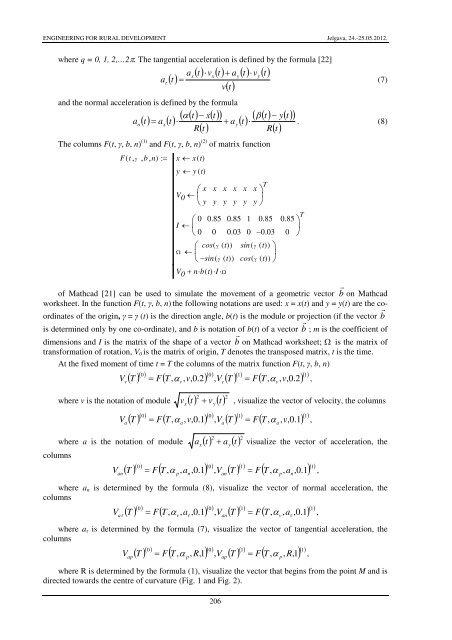
ENGINEERING FOR RURAL DEVELOPMENT Jelgava, 24.-25.05.2012.where q = 0, 1, 2,…2π. The tangential acceleration is defined by the formula [22]( t) ⋅vx( t) + ay( t) ⋅ vy( t)v( t)and the normal acceleration is defined by the formula( ) ( )( α( t) − x( t))ant = axt ⋅ + ayR taxaτ ( t)=(7)( )206( t)The columns F(t, γ, b, n) (1) and F(t, γ, b, n) (2) of matrix functionF( t , γ , b , n) := x ← x( t)y ←y ( t)⎛V 0 ← ⎜⎝⎛I ← ⎜⎝Ω←⎛⎜⎝00xyxy0.850xycos( γ ( t))xy0.850.03−sin( γ ( t))V 0 + n⋅b( t)⋅I⋅Ωxy⋅10( β ( t) − y( t))R( t)Tx ⎞⎟y ⎠0.85−0.03sin( γ ( t)) ⎞ ⎟⎠cos( γ ( t))T0.85 ⎞ ⎟⎠0. (8)of Mathcad [21] can be used to simulate the movement of a geometric vector b r on Mathcadworksheet. In the function F(t, γ, b, n) the following notations are used: x = x(t) and y = y(t) are the coordinatesof the origin, γ = γ (t) is the direction angle, b(t) is the module or projection (if the vector b ris determined only by one co-ordinate), and b is notation of b(t) of a vector b r ; m is the coefficient ofdimensions and I is the matrix of the shape of a vector b r on Mathcad worksheet; Ω is the matrix oftransformation of rotation, V 0 is the matrix of origin, T denotes the transposed matrix, t is the time.At the fixed moment of time t = T the columns of the matrix function F(t, γ, b, n)columnsVv( T ) ( 0) F( T, α , v,0.2) ( 0), V ( T ) ( 1)= F( T,α , v,0.2 ) ( 1)where v is the notation of module ( ) ( ) 2Va= ,vv2vytvvx t + , visualize the vector of velocity, the columns( T ) ( 0) F( T, α , v,0.1) ( 0), V ( T ) ( 1)= F( T,α , v,0.1 ) ( 1)= ,where a is the notation of module ( ) ( ) 2Vanaa2 aytaax t + visualize the vector of acceleration, the( T ) ( 0) F( T α , a ,0.1) ( 0), V ( T ) ( 1)= F( T,α , a ,0. 1 ) ( 1)= ,,p nanp nwhere a n is determined by the formula (8), visualize the vector of normal acceleration, thecolumnsV( T ) ( 0) F( T α , a ,0.1) ( 0), V ( T ) ( 1)F( T,α , a ,0. 1 ) ( 1)a τ,v τan=v τ= ,where a τ is determined by the formula (7), visualize the vector of tangential acceleration, thecolumnsVap( T ) ( 0) F( T, α , R,1) ( 0), V ( T ) ( 1)= F( T,α , R,1 ) ( 1)= ,pwhere R is determined by the formula (1), visualize the vector that begins from the point M and isdirected towards the centre of curvature (Fig. 1 and Fig. 2).app