Aare Aan, Mati Heinloo Estonian University of Life Sciences ...

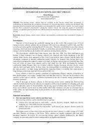
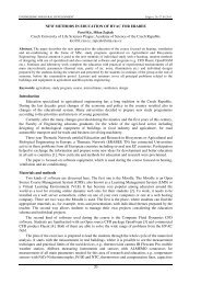
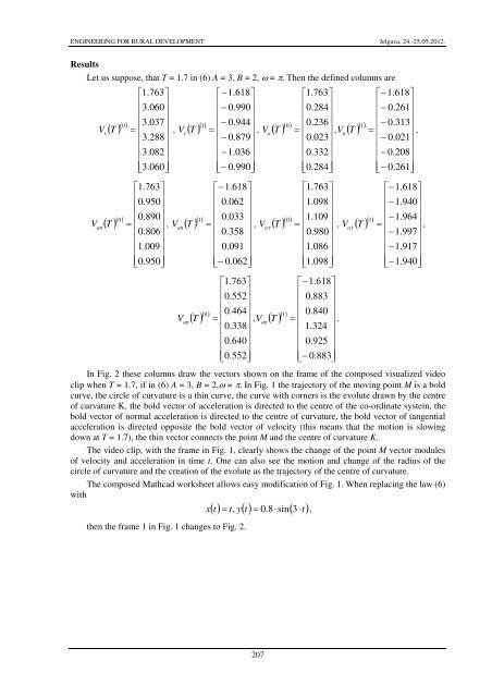
ENGINEERING FOR RURAL DEVELOPMENT Jelgava, 24.-25.05.2012.ResultsLet us suppose, that T = 1.7 in (6) A = 3, B = 2, ω = π. Then the defined columns are⎡1.763⎤⎢⎢3.060⎢3.037( ) ( 0V ) vT = ⎢ , ( ) ( 1V ) vT = ⎢ , ( ) ( 0V ) aT = ⎢ , ( ) ( 1T) = ⎢⎢3.288⎢−0.879⎢0.023⎢−0.021⎢3.082⎢3.060⎥ ⎥⎥⎥⎥⎥⎥⎥ ⎢−1.036⎢⎦− 0.990⎥ ⎥⎥⎥⎥⎥⎥⎥ ⎢0.332⎢⎦0.284⎥ ⎥⎥⎥⎥⎥⎥⎥ ⎢−0.208⎢⎦− 0.261⎥ ⎥⎥⎥⎥⎥⎥⎥ ⎦⎣⎡1.763⎤⎢⎢0.950⎢0.890⎡−1.618⎤⎢⎢− 0.990⎢−0.944⎣⎡1.763⎤⎢⎢0.284⎢0.236⎣⎡−1.618⎤⎢⎢− 0.261⎢−0.313V a,( ) ( 0V ) anT = ⎢ , ( ) ( 1V ) anT = ⎢ , ( ) ( 0V ) aτT = ⎢ , ( ) ( 1T) = ⎢⎢0.806⎢ 0.358⎢0.980⎢−1.997⎢1.009⎢0.950⎥ ⎥⎥⎥⎥⎥⎥⎥ ⎢ 0.091⎢⎦− 0.062⎥ ⎥⎥⎥⎥⎥⎥⎥ ⎢1.086⎢⎦1.098⎥ ⎥⎥⎥⎥⎥⎥⎥ ⎢−1.917⎢⎦−1.940⎥ ⎥⎥⎥⎥⎥⎥⎥ ⎦⎣⎡−1.618⎤⎢⎢0.062⎢ 0.033⎣⎡1.763⎤⎢⎢0.552⎢0.464⎡1.763⎤⎢⎢1.098⎢1.109( ) ( 0V ) apT = ⎢ , ( ) ( 1T) = ⎢⎢0.338⎢ 1.324⎢0.640⎢0.552⎥ ⎥⎥⎥⎥⎥⎥⎥ ⎢ 0.925⎢⎦− 0.883⎥ ⎥⎥⎥⎥⎥⎥⎥ ⎦⎣⎡−1.618⎤⎢⎢0.883⎢ 0.840V ap.⎣⎣⎣⎡−1.618⎤⎢⎢−1.940⎢−1.964V aτ,In Fig. 2 these columns draw the vectors shown on the frame of the composed visualized videoclip when T = 1.7, if in (6) A = 3, B = 2,ω = π. In Fig. 1 the trajectory of the moving point M is a boldcurve, the circle of curvature is a thin curve, the curve with corners is the evolute drawn by the centreof curvature K, the bold vector of acceleration is directed to the centre of the co-ordinate system, thebold vector of normal acceleration is directed to the centre of curvature, the bold vector of tangentialacceleration is directed opposite the bold vector of velocity (this means that the motion is slowingdown at T = 1.7), the thin vector connects the point M and the centre of curvature K.The video clip, with the frame in Fig. 1, clearly shows the change of the point M vector modulesof velocity and acceleration in time t. One can also see the motion and change of the radius of thecircle of curvature and the creation of the evolute as the trajectory of the centre of curvature.The composed Mathcad worksheet allows easy modification of Fig. 1. When replacing the law (6)withthen the frame 1 in Fig. 1 changes to Fig. 2.x( t) = t y( t) = 0.8⋅sin( 3⋅t), ,⎣207