Static analysis of cable structures 1. Introduction Cable structures ...
Static analysis of cable structures 1. Introduction Cable structures ...
Static analysis of cable structures 1. Introduction Cable structures ...

You also want an ePaper? Increase the reach of your titles
YUMPU automatically turns print PDFs into web optimized ePapers that Google loves.
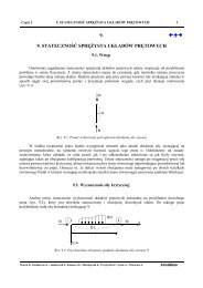
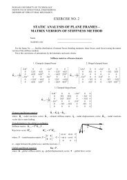
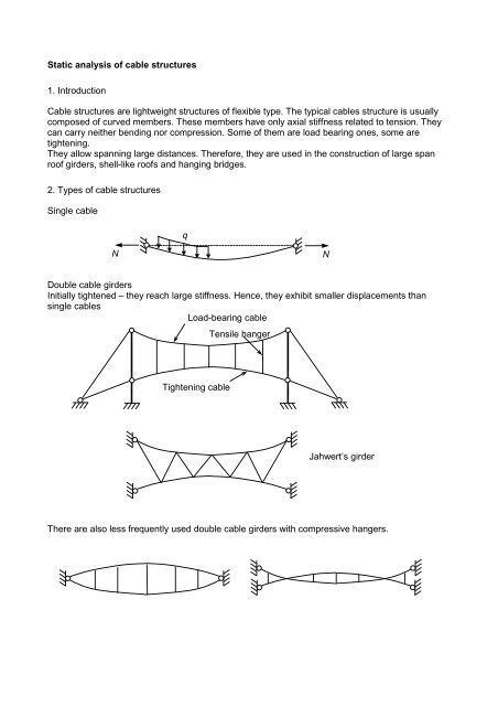
<strong>Static</strong> <strong>analysis</strong> <strong>of</strong> <strong>cable</strong> <strong>structures</strong><strong>1.</strong> <strong>Introduction</strong><strong>Cable</strong> <strong>structures</strong> are lightweight <strong>structures</strong> <strong>of</strong> flexible type. The typical <strong>cable</strong>s structure is usuallycomposed <strong>of</strong> curved members. These members have only axial stiffness related to tension. Theycan carry neither bending nor compression. Some <strong>of</strong> them are load bearing ones, some aretightening.They allow spanning large distances. Therefore, they are used in the construction <strong>of</strong> large spanro<strong>of</strong> girders, shell-like ro<strong>of</strong>s and hanging bridges.2. Types <strong>of</strong> <strong>cable</strong> <strong>structures</strong>Single <strong>cable</strong>qNNDouble <strong>cable</strong> girdersInitially tightened – they reach large stiffness. Hence, they exhibit smaller displacements thansingle <strong>cable</strong>sLoad-bearing <strong>cable</strong>Tensile hangerTightening <strong>cable</strong>Jahwert’s girderThere are also less frequently used double <strong>cable</strong> girders with compressive hangers.
Pylons may have various cross-sections– masts with guysMastGuy (<strong>cable</strong>)3. Basic equation for a single <strong>cable</strong>Let us consider a single <strong>cable</strong> subjected to the axial tightening force and transverse loading.NAqlR A =2flCqlR B =2qBNSince the <strong>cable</strong> carries no bending we can write down the equation <strong>of</strong> equilibrium <strong>of</strong> moments withrespect to the centre point C for a half <strong>of</strong> the <strong>cable</strong>∑ql l ql lNf − ⋅ + ⋅2 2 2 4M leftC =and get the basic relation between the tightening force and the uniform transverse loading2qlN = 8 f0
where the transformation matrix isKe= TTe~KeTeThe direction cosine c ab is defined asT⎡C0⎤T e = ⎢ ⎥ with⎣0C ⎦⎡c⎢C = ⎢c⎢⎣c( a , b)~c ab = cos ∠The first part <strong>of</strong> the element stiffness matrix can be transformed as followsT⎡CK1e= ⎢⎣ 0⎡ T ~C Kii= ⎢T ~⎢⎣− C K1, eii1,e⎡ ~0 ⎤ Kii1,e⎥⎢T ~C ⎦⎢⎣− Kii1,T ~C − C KT ~C C Keii1,ii1,e~− K~K⎤eC⎥C ⎥⎦and similarly for the second part we getKii1,eii1,e⎤⎡C⎥⎢⎥⎦⎣0⎡ T ~C Kii= ⎢T ~⎢⎣− C Kxxyxzx⎡T ~0⎤C Kii⎥ = ⎢T ~C⎦⎢⎣− C KCT ~− C K2, eii 2,2 eT ~ii 2, eCC Kii2, eWe can substitute the explicit form <strong>of</strong> the matrices and get1, eii1,eccc⎤eC⎥C ⎥⎦xyyyzycccxzyzzz⎤⎥⎥⎥⎦T ~− C KT ~C Kii1,eii1,e⎤⎡C⎥⎢⎥⎦⎣00⎤⎥ =C⎦T ~C K=ii1,eC =2⎡ cxxEA ⎢⎢cxxcL0⎢⎢c⎣xxcEALyxzx0⎡c⎢⎢c⎢⎣ccxx yx2cyxczxxxyxzxccyxcccxyyyzyccxxccccczxxzyzzzzx yx2czx⎤⎡1⎥⎢⎥⎢0⎥⎦⎢⎣0⎤⎥⎥⎥⎥⎦0000⎤⎡c⎥⎢0⎥⎢c0⎥⎦⎢⎣cxxxyxzcccyxyyyzccczxzyzz⎤⎥⎥ =⎥⎦EAL0⎡c⎢⎢c⎢⎣cxxyxzx0000⎤⎡c⎥⎢0⎥⎢c0⎥⎦⎢⎣cxxxyxzcccyxyyyzccczxzyzz⎤⎥⎥ =⎥⎦T ~C K=NLii 2, e⎡⎢⎢⎢⎢⎣C =NL⎡c⎢⎢c⎢⎣cxxyxzxcccxyyyzycccxzyzzz⎤⎡0⎥⎢⎥⎢0⎥⎦⎢⎣00⎤⎡c⎥⎢0⎥⎢c1⎥⎦⎢⎣c⎤⎥⎥ =⎥⎦2 2( c ) ( ) ( ) ⎤xy + cxzcxycyy+ cxzcyz cxyczy+ cxzczz2 2( cxycyy+ cxzcyz) ( cyy+ cyz) ( cyyczy+ cyzczz)2 2( c + ) ( + ) ( + ) ⎥ ⎥⎥⎥ xy czycxzczzcyyczycyzczzczyczz⎦010xxxyxzThe elements <strong>of</strong> the second submatrix can be rewritten if the orthogonality conditions for thedirection cosines are used. We have for instance:cccyxyyyzccczxzyzzNL⎡0⎢⎢0⎢⎣0cccxyyyzycccxzyzzz⎤⎡c⎥⎢⎥⎢c⎥⎢⎦⎣cxxxyxzcccyxyyyzccczxzyzz⎤⎥⎥ =⎥⎦c2 2 2xx + cxy+ cxz= 1so the first diagonal term can be given asc2xy+ c2xz=21−cxxThere is also
cxxcyx+ cxycyy+ cxzcyz= 0so the first <strong>of</strong>f-diagonal term can be given ascxycyy+ cxzcyz= −cxxcyxUsing the similar relations the entire second part <strong>of</strong> the stiffness matrix can be rewritten and finallywe getKe⎡ Kii= ⎢⎣−K1, eii1,e− KKii1,eii1,e⎤ ⎡ Kii⎥ + ⎢⎦ ⎣−K2, eii 2, e− KKii 2, eii 2, e⎤⎥⎦where:KKii 2, eii1,e==NL2⎡ cxxEA ⎢⎢cxxcL0⎢⎢c⎣xxcyxzx2( 1−c )⎡⎢⎢−c⎢⎢−c⎣xxxxxxccyxzxcxx yx2cyxc− czxccyxxx yx2( 1−cyx)− cyxcczxccxxcczxzx yx2czx− c− cxx⎤⎥⎥⎥⎥⎦cczx⎤yx zx( )⎥ ⎥⎥ 21−czx⎥ ⎦Thus we have expressed the stiffness matrix in terms <strong>of</strong> direction cosines between the local axis x ~and the global axes x, y and z. Because <strong>of</strong> such a relatively simple form, usually the elementmatrices are directly given in the global co-ordinates using the co-ordinates <strong>of</strong> nodes. Let usconsider the elementxyx iz iy iiy kx ke z Lkkzx ~The cosines required to express the element stiffness matrix can be given ascccxxyxzx= cos ∠= cos ∠= cos ∠( x,x~ )( y,x~ )( z,x~ )xk− xi=Ly k − y i=Lzk− zi=LThus, with these definitions there is no necessity for the transformation <strong>of</strong> co-ordinates.After the assembly <strong>of</strong> the global stiffness matrix K and inclusion <strong>of</strong> support conditions the global set<strong>of</strong> equations is formulatedKq = PThe global stiffness matrix has the dimension n×n, where n = 3s and s is the number <strong>of</strong> free(unsupported) nodes.
Solution <strong>of</strong> this equation gives the nodal displacements in the vector q. Then the equilibriumconditions in the deformed configuration must be checked.The new co-ordinates <strong>of</strong> nodes are obtained fromx ' = x + uiy ' = yiiz ' = z + wx ' = xkkkiikiky ' = ykz ' = zand the displacements u i , v i and w i come from q.The current length <strong>of</strong> the element is:i+ vii+ u+ vk+ wkkso the length increment isL'=( x ' −x') 2 + ( y ' −y') 2+ ( z ' −z' ) 2kikiki∆ L'=The current value <strong>of</strong> the axial force in the element is222( xk' −xi') + ( y k ' −yi ') + ( zk' −zi') − L0N' = N + ∆N'where the current force increment is obtained from the Hooke’s law∆L'∆ N'= EA Having found the current axial forces we can calculate the out-<strong>of</strong>-balance nodalL0forces ∆Q x ', ∆Q y ' and ∆Q z ' assembled into a vectorQ y 'Q x ' x⎡∆Qx' ⎤m⎢ ⎥∆Q ' =⎢∆Qy'Q⎥z 'N r 'N r ' = −∑N e ' ce = 1⎢⎣∆Q' ⎥yz ⎦Let us denote the resultant from the axial forces in the m-elements coinciding at a node as N r '.Then, using the equilibrium conditions at the node we getor in the matrix notationwhere⎡Q⎢Q ' =⎢Q⎢⎣Qxyz' ⎤⎥'⎥' ⎥⎦Q ' +xQ ' +yQ ' +zzm∑e = 1m∑e = 1m∑e = 1N ' cos ∠eN ' cos ∠eN ' cos ∠eQ ' = −⎡cos∠⎢c = ⎢cos∠⎢⎣cos∠m∑ N ee = 1( x,x~ )( y,x~)= 0= 0( z,x~ ) = 0' c( x,x~) ⎤ ⎡cxx ⎤⎥( )⎢y,x~⎥ =⎢cyx( ) ⎥ ⎢ ⎥ ⎥⎥ z,x~⎣czx⎦⎦
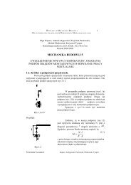
The external forces at the nodes areP ' P + P= 0where P 0 is the vector <strong>of</strong> initial (tightening) nodal forces and P is the vector <strong>of</strong> external imposedloads.The out-<strong>of</strong>-balance forces arem0 ∑N e 'e=1∆Q'= P'−Q'= P + P +In the next iteration the equilibrium equation readsK'∆ q'= ∆Q'Solving <strong>of</strong> these equations yields the vector <strong>of</strong> displacement increments, which are used tocalculate the new values <strong>of</strong> current displacementsq' = q + ∆q'From this point the calculations are repeated to get the new values <strong>of</strong> out-<strong>of</strong>-balance forces, etc.The iterations stop when the current value <strong>of</strong> the out-<strong>of</strong>-balance forces falls below a tolerance∆Q ' ≤ tolcThe presented algorithm follows the line <strong>of</strong> the Newton method. Let us now briefly present themethods <strong>of</strong> iterative solving <strong>of</strong> non-linear equations.The Newton methodP∆Q'- a new stiffness matrix at each iterationPQ'qq ∆q' ∆q''q realThe modified Newton methodPP∆Q'Q'q∆q'q realq- the initial stiffness matrix used at eachiteration- slower convergence but low computationcost at each iteration
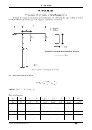
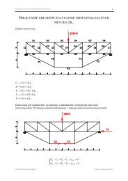
The Newton-Raphson methodPP 3P 2P- loading divided into increments- much better convergence in highly nonlinearcasesP 1q5. ExampleWe consider a plane <strong>cable</strong> system consisting <strong>of</strong> 3 elements.Initial configurationHAR Ay1xCP 02DP 033 4 3BR BH3Node co-ordinates:x A = 0.0y A = 0.0x B = 10.0y B = 0.0x C = 3.0y C = 3.0x D = 7.0y D = 3.0Data:EA = 8000 kNInitial tightening load – two nodal forces P 0 = 5 kNThe reactions in the initial configuration are∑M B∑: 10R− 5 ⋅ 7 − 5 ⋅ 3 = 0 ⇒ RAM CA =∑y : RB = 5kN: 3RA − 3H= 0 ⇒ H = 5kNThe axial forces in the inclined <strong>cable</strong>s can be obtained from the equilibrium <strong>of</strong> the node A or B5kNHAR AN 1∑2y : N = 5kN ⇒ N121 =7.07107kNAnd from the symmetry N 3 = N 1 .The force in the <strong>cable</strong> CD comes from the equilibrium <strong>of</strong> the node CN 1 CN 2P 0∑x22: N1 = N2⇒ N2=5kN
The <strong>cable</strong> system in this configuration is now loaded by a set <strong>of</strong> two external loads P = 12 kNA xBH13H3R AC 2 DR ByP 0P 0P P3 4 3Initial lengths for the elements are22( 3 − 0) + ( 3 − 0) = 4.24264 L0,3L =0,1=mThe direction cosines are:ccLxx,1yx,122( 7 − 3) + ( 3 − 3) 4.0m0 ,2 ==xC− x=Ly=C0,1− yL0,1AA3 − 0= = 0.7071074.242643 − 0= = 0.7071074.24264ccxx,2yx,2xD− x=L0,2yD− y=L0,2CC7 − 3= = <strong>1.</strong>04.03 − 3= = 0.04.0The element stiffness matricesK=AA,1=EAL0,180004.24264⎡0.5⎢⎣0.5cc⎡ c⎢⎢⎣cxxcxx,3yx,32xx,1,1 yx,1xB− x=L0,3yB− y=Lc0.5⎤⎥ +0.5⎦K0,31DD10 − 7= = 0.7071074.24264⎡ K= ⎢⎣−Kcxx,1yx,12cyy,10 − 3= = −0.7071074.24264AA,1AA,1⎤ N⎥ +⎥⎦L7.071074.2426410,1⎡ 0.5⎢⎣−0.5− KKAA,1AA,1⎤⎥⎦2( 1−c )⎡⎢⎢⎣− cxx,1cxx,1yx,1− ccxx,1yx,12( 1−cyy,1)− 0.5⎤⎡943.643⎥ = ⎢0.5 ⎦ ⎣94<strong>1.</strong>976⎤⎥ =⎥⎦94<strong>1.</strong>976⎤⎥943.643⎦K2⎡ K= ⎢⎣−KAA,2AA,2− KKAA,2AA,2⎤⎥⎦
K=AA,2=EAL0,28000 ⎡1⎢4.0 ⎣0⎡ c⎢⎢⎣cxx0⎤⎥ +0⎦2xx,2c,2 yx,254.0⎡0⎢⎣0ccxx,2yx,22cyy,2⎤ N⎥ +⎥⎦L20,20⎤⎡2000.0⎥ = ⎢1⎦⎣ 02( 1−c )⎡⎢⎢⎣− cxx,20 ⎤⎥<strong>1.</strong>250⎦xx,2cyx,2− ccxx,2yx,22( 1−cyy,2)⎤⎥ =⎥⎦K=AA,3=EAL0,380004.24264⎡ c⎢⎢⎣cxx⎡ 0.5⎢⎣−0.52xx,3c,3 yx,3cK− 0.5⎤⎥ +0.5 ⎦3c⎡ K= ⎢⎣−Kxx,3yx,32cyy,3AA,3AA,3⎤ N⎥ +⎥⎦L7.071074.2426430,3⎡0.5⎢⎣0.5− KKAA,3AA,3⎤⎥⎦2( 1−c )⎡⎢⎢⎣− cxx,3xx,3cyx,3− ccxx,3yx,32( 1−cyy,3)0.5⎤⎡ 943.643⎥ = ⎢0.5⎦⎣−94<strong>1.</strong>976⎤⎥ =⎥⎦− 94<strong>1.</strong>976⎤⎥943.643 ⎦The pattern <strong>of</strong> global stiffness matrix assembly and support conditions inclusion isK =ACDBA C D BK 1K 2K 3and the remaining fragment <strong>of</strong> the matrix K corresponds to the free nodes C and D.This remaining fragment is⎡2943.64⎢⎢94<strong>1.</strong>976K =⎢−2000.0⎢⎣ 0.094<strong>1.</strong>976944.8930.0−<strong>1.</strong>250− 2000.00.02943.64− 94<strong>1.</strong>9760.0 ⎤⎥−<strong>1.</strong>250⎥− 94<strong>1.</strong>976⎥⎥944.893 ⎦The load vector corresponding to the free nodes C and D has two forces P in the y direction andzero forces in the x directionThe solution <strong>of</strong> the equilibrium equation⎡ 0.0 ⎤⎢ ⎥⎢12.0P = ⎥⎢ 0.0 ⎥⎢ ⎥⎣12.0⎦Kq = P is⎡− 0.0029922⎤⎢⎥⎢0.0157036q =⎥⎢ 0.0029922 ⎥⎢⎥⎣ 0.0157036 ⎦Now we can find the new co-ordinates <strong>of</strong> free nodes
The current element lengths arexyyCCDD' = 3.0 − 0.0029922 = 2.99701' = 3.0 + 0.0157036 = 3.01570x ' = 7.0 + 0.0029922 = 7.00299' = 3.0 + 0.0157036 = 3.0157022( 2.99701−0.0) + ( 3.01570 − 0.0) = 4.25165m 'L =1' =L322( 7.00299 − 2.99701) + ( 3.01570 − 3.01570) 4.00598mL 2 ' ==The length increments are∆ L 0,1'= 4.25165 − 4.24264 = 0.00901m= ∆L0,3'∆ L 0 ,2 ' = 4.00598 − 4.0 = 0.00598mThe increments <strong>of</strong> axial forces∆L0,1'0.00901∆ N1' = EA = 8000 ⋅ = 16.9894kN = ∆N3'L4.24264∆N0,1∆L' = EAL' 0.00598= 8000 ⋅4.00,22 =0,21<strong>1.</strong>9680kNand the current values <strong>of</strong> the axial forcesN 1' = N1+ ∆N1'= 7.07107 + 16.9894 = 24.0605kN = N3'N ' = N + ∆N2 ' = 5.0 + 1<strong>1.</strong>96802 2=The current values <strong>of</strong> the direction cosines areccccxx,1yx,1xx,3yx,32.99701−0== 0.7049054.251653.01570 − 0== 0.7093014.25165ccxx,2yx,2= <strong>1.</strong>0= 0.016.9680kN10 − 7.00299== 0.7049054.251650 − 3.01570== −0.7093014.25165The out-<strong>of</strong>-balance forces can be found from the equilibrium <strong>of</strong> nodes24.0605 C16.96805 + 12x∆Q∆Qxy' = −24.0605⋅ 0.704905 + 16.9680 = 0.00763kN' = −24.0605⋅ 0.709301+12 + 5 = −0.06614kNy
And similarly, from the equilibrium <strong>of</strong> the node D we getto complete the vector∆Q∆Qxy' = −0.00763kN' = −0.06614kN⎡ 0.00763 ⎤⎢ ⎥⎢− 0.06614∆Q' =⎥⎢−0.00763⎥⎢ ⎥⎣−0.06614⎦The stiffness matrices in the current configuration are formed using the following submatricesK=K=EA ⎡ c= ⎢L0,1⎢⎣cxx8000 ⎡0.496891⎢4.24264 ⎣ 0.50⎤ N ⎡1'⎥ + ⎢⎥⎦L1'⎢⎣− c2( 1−c )2xx,1cxx,1cyx,1xx,1− c cAA,1' 22,1cyx,1cyy,1xx,1cyx,1⎡⎢⎣K=EA ⎡ c= ⎢L0,3⎢⎣cxx80004.24264xx,1yx,1( 1−cyy,1)0.50 ⎤ 24.0605 ⎡0.503108⎥ + ⎢0.503108⎦4.25165 ⎣ − 0.50EA ⎡ c= ⎢L0,2⎢⎣cxx8000 ⎡1⎢4.0 ⎣00⎤⎥ +0⎦16.96804.00598⎡0⎢⎣0⎤ N ⎡2'⎥ + ⎢⎥⎦L2' ⎢⎣− c0⎤⎡2000.0⎥ = ⎢1⎦⎣ 0⎤⎥ =⎥⎦− 0.50 ⎤ ⎡939.794⎥ = ⎢0.496891⎦⎣939.9802( 1−c )2xx,2cxx,2cyx,2xx,2− c cAA,2' 22,2cyx,2cyy,2xx,2cyx,20.496891− 0.50⎤ N ⎡3'⎥ + ⎢⎥⎦L3' ⎢⎣− c2( 1−c )2xx,3cxx,3cyx,3xx,3− c cAA,3 '22,3cyx,3cyy,3xx,3cyx,3− 0.50 ⎤ 24.0605 ⎡0.503108⎥ + ⎢0.503108⎦4.25165 ⎣ 0.50xx,3yx,3( 1−cyy,3)0 ⎤⎥4.23567⎦⎤⎥ =⎥⎦xx,2yx,2( 1−cyy,2)⎤⎥ =⎥⎦0.50 ⎤ ⎡ 939.794⎥ = ⎢0.496891⎦⎣−939.980939.980⎤⎥95<strong>1.</strong>482⎦− 939.980⎤⎥95<strong>1.</strong>482 ⎦Following the same assembly and support conditions pattern we get the “active” part <strong>of</strong> the globalstiffness matrix in the form⎡2939.79⎢⎢939.980K ' =⎢−2000.0⎢⎣ 0.0939.980955.7180.0− 4.23567− 2000.00.02939.79− 939.980and solving the equilibrium equations with out-<strong>of</strong>-balance forceswe get the following increments <strong>of</strong> displacementsK'∆ q'= ∆Q'⎡ 0.0000182 ⎤⎢⎥⎢− 0.0000875∆q' =⎥⎢−0.0000182⎥⎢⎥⎣−0.0000875⎦With these values the total current displacements can be found0.0 ⎤⎥− 4.23567⎥− 939.980⎥⎥955.718 ⎦
⎡u⎢⎢v⎢u⎢⎣vCCDD' ⎤ ⎡−0.0029922 + 0.0000182⎤⎡− 0.0029738⎤⎥'⎢⎥ ⎢⎥⎥ ⎢0.0157037 − 0.0000852⎥ = ⎢0.0156162= ∆q'+ q =⎥' ⎥ ⎢ 0.0029922 − 0.0000182 ⎥ ⎢ 0.0029738 ⎥⎥ ⎢⎥ ⎢⎥' ⎦ ⎣ 0.0157037 − 0.0000852 ⎦ ⎣ 0.0156162 ⎦The co-ordinates <strong>of</strong> nodes in the current deformed configurationThe current element lengths areThe length increments areThe increments <strong>of</strong> axial forcesand the current values <strong>of</strong> the axial forcesxyyCCDD' ' = 3.0 − 0.0029738 = 2.997026' ' = 3.0 + 0.0156162 = 3.016162x ' ' = 7.0 + 0.0029738 = 7.002974''= 3.0 + 0.0156162 = 3.016162L 1' ' = 4.251600m = L3''L 2 ' ' =4.005948m∆ L0 ,1' ' = 0.008960m = ∆L0,3''∆L 0 ,2 ' ' =0.005948m∆ N1' ' = 16.8951kN = ∆N3''∆N''2 =The current values <strong>of</strong> the direction cosines are1<strong>1.</strong>8960kNN 1' ' = N1+ ∆N1'' = 23.9662kN = N3''N 2 ''= N2+ ∆N2'' = 16.8960kNccxx,1yx,1cc= 0.704917= 0.709290xx,2yx,2= <strong>1.</strong>0= 0.0ccxx,3yx,3= 0.704917= −0.709290The current out-<strong>of</strong>-balance forces can be found from the equilibrium <strong>of</strong> nodes23.9662 C16.89605 + 12x∆Q∆Qxy''= −23.9662⋅ 0.704917 + 16.8960 = 0.00182kN''= −23.9662⋅ 0.709290 + 12 + 5 = 0.00101kNy
These values are several times smaller than the out-<strong>of</strong>-balance forces in the first iteration, whatconfirms the convergence behaviour <strong>of</strong> the solution process.They are also relatively small compared to the current values <strong>of</strong> forces in the elements (about0.001%), so the iterations can be stopped at this point.