Time Series Exam, 2009: Solutions - STAT

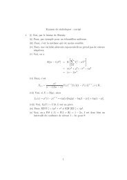
pure sAR(P): ACF tailing off, PACF cuts off after lag sP;pure sMA(Q): ACF cuts off after lag sQ, PACF tailing off.The ordinary ARMA pattern is (approximately) repeated at everyns lags (n integer) if there is a seasonal component. For a morecomplex model, whenever AR and MA or sAR and sMA terms areboth present, the ACF and PACF is much less clear, and severalpossible models should be fitted and compared.Model estimation: Fit oneor severalSARIMA model to the stationarizeddata. The method can be generallymaximum likelihood. Models canbe compared by their predictive error, AIC or BIC; the best modelis where the value of the chosen criterion is the smallest. AIC andBICpenalize thenumber ofintroducedparametersinthe model; AICtends to choose slightly overfitted models.Model diagnostics: Theperformanceofthechosenmodelmustbechecked.Parameters: Likelihood ratio tests to check if the model is adequatecompared to more complex models, and whether it is not unnecessarilycomplex compared to simpler models;QQ plot of the residuals: To check the distributional assumption ofour model for the errors;Periodogram of the residuals: To check if the residuals are indeedwhite noise;ACF and PACF of the residuals, Ljung-Box test: Other tests todetect remaining significant correlations in the residuals.Prediction: The best linear predictor Ỹn+h for an ARMA model isỸ n+h =∞∑ψ j ǫ n+h−j ,j=hwhereψ j arethecoefficientsofthegenerallinearrepresentationoftheprocess. The ǫ i are taken as the estimated residuals for i = 1,...,nand zero for i = n+1,...,n+h.The estimated ARMA (or SARIMA) parameters can also be used.Fornonstationarydata(stationarizedbydifferencingandfitted afterwards)this will predict the differenced sequence; to obtain predictionon the original scale, we must use the appropriate backward transformation.6. The estimator of γ XY (h) based on data (X 1 ,Y 1 ),...,(X n ,Y n ) isˆγ XY (h) = 1 n−h∑(X t+h −n¯X)(Y t −Ȳ).t=1A corresponding expression can be given as the estimator of the crosscorrelationρ XY (h). ˆγ XY (h) and ˆρ XY (h) are consistent and asymptoticallyunbiased for γ XY (h) and ρ XY (h), under conditions similar to thoseforthegoodbehaviouroftheunivariatecorrelogram. Fortwouncorrelatedwhite noise series for large n,E{ˆρ XY (h)} . = 0 and var{ˆρ XY (h)} . = n −1 .In the case of uncorrelated series which are not white noise, the estimatorˆρ XY (h) can show significant cross-correlations despite the uncorrelatedness.In such a case, fit marginal models to the sequences, and examinethe cross-correlation of the residuals (pre-whitening).(a) The models can be written asX t = ǫ t +θ 11 ǫ t−1 +θ 12 η t−1 ,Y t = η t +θ 21 ǫ t−1 +θ 22 η t−1 ,4