Time Series Exam, 2009: Solutions - STAT

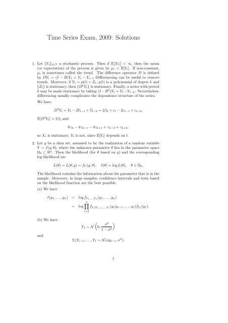
Time Series Exam, 2009: Solutions1. Let {Y t } t∈T a stochastic process. Then if E[|Y t |] < ∞, then the mean(or expectation) of the process is given by µ t = E[Y t ]. If non-constant,µ t is sometimes called the trend. The difference operator D is definedby DY t = (I − B)Y t = Y t − Y t−1 Differenceing can be useful to removetrends. Moreover, if Y t = p(t)+Z t , p(t) is a polynomial of degree k and{Z t } is stationary, then {D k Y t } is stationary. Finally, a series with periodk may be made stationary by taking (I−B k )Y t = Y t −Y t−k . Nevertheless,differencing usually complicates the dependence structure of the series.We haveE[D 2 Y t ] = 2β 2 andD 2 Y t = Y t −2Y t−1 +Y t−2 = 2β 2 +ε t −2ε t−1 +ε t−2 ,6γ h −4γ h−1 −4γ h+1 +γ h−2 +γ h+2 ,so X t is stationary. Y t is not, since E[Y t ] depends on t.2. Let y be a data set, assumed to be the realization of a random variableY ∼ f(y;θ), where the unknown parameter θ lies in the parameter spaceΩ θ ⊂ R d . Then the likelihood (for θ based on y) and the correspondinglog likelihood areL(θ) = L(θ;y) = f Y (y;θ), l(θ) = logL(θ), θ ∈ Ω θ .The likelihood contains the information about the parameterthat is in thesample. Moreover, in large samples, confidence intervals and tests basedon the likelihood function are the best possible.(a) We havel(y 1 ,...,y n ) = logf Y1,...,Y n(y 1 ,...,y n )n∏= log f Yi|Y i−1,...,Y 1(y i |y i−1 ,...,y 1 )f Y1 (y 1 ).i=2(b) We haveandY 1 ∼ NÅσ 2 ã0,1−φ 2Y i |Y i−1 ,...,Y 1 ∼ N(φy i−1 ,σ 2 ).1

So,l(σ 2 ,φ) = − 1 2 log(2πσ2 /(1−φ 2 ))− 1 2 y2 1(1−φ 2 )/σ 2which gives the desired result.−(n−1) 1 2 log(2πσ2 )− 1 2n∑(y i −φy i−1 ) 2 /σ 2 ,(c) (i)To get confidence intervals for φ and σ 2 , we need to compute ˆφ andˆσ 2 , the maximum likelihood estimates, using the log likelihood function.Then, we can compute (1−2α) confidence intervals for these parametersas ˆφ±z α v 1/211 and ˆσ2 ±z α v 1/222 , where v ii is the ith diagonal element of thematrix J((ˆφ,ˆσ 2 )) −1 .(ii) The likelihood ratio statistic for comparing the model with φ ∈ R withthe model with φ = 0 is W = 2(ˆl φ − ˆl φ=0 ). If the hypothesis φ = 0 istrue, then W ∼ χ 2 1 .3. If {γ h } h∈Z is the ACF of a stationary random sequence, then there existsa unique function F defined on [−1/2,1/2] such that F(−1/2) = 0, Fis right-continuous and non-decreasing, with symmetric increments aboutzero, and ∫γ h = e 2πihu dF(u), h ∈ Z.(−1/2,1/2]The function F is called the spectral distribution function of γ h , andits derivative f, if it exists, is called the spectral density function. If∑h |γ h| < ∞, then f exists. A function f(ω) defined on [−1/2,1/2] is thespectrum of a stationary process if and only if f(ω) = f(−ω), f(ω) ≥ 0,and ∫ f(ω)dω < ∞.We haveγ YY (h) = E[(Y t+h −E[Y t+h ])(Y t −E[Y t ])]ñ ô∑ ∑= E ψ r (ε t+h−r −E[ε t ])(ε t−s −E[ε t ])ψ sr s= ∑ ∑ψ r γ εε (h−r +s)ψ sr s= σ 2∑ ∑ψ r δ(h−r+s)ψ s ,r si=2hence,f(ω) = σ 2∑ h= σ 2∑ r∑∑ψ r δ(h−r+s)ψ s e −2πiωhr sψ r e −2πiωr∑ ψ s e 2πiωss= σ 2 |ψ(ω)| 2 .Finally, we havef(ω) = σ 2( 1+θe −2πiω)( 1+θe 2πiω) = σ 2 (1+θ 2 +2θcos(2πω)).4. A time series {Y t } is an autoregressive-moving average process of orderp,q, ARMA(p,q), model, if it is stationary and of the formY t = φ 1 Y t−1 +φ 2 Y t−2 +···+φ p Y t−p +ε t +θ 1 ε t−1 +···+θ q ε t−q ,where φ 1 ,...,φ p ,θ 1 ,...,θ q are constants with φ p ,θ q ≠ 0, and v t is whitenoise.2

An ARMA(p,q) process φ(B)Y t = θ(B)ε t is causal if it can be written asa linear process∞∑Y t = ψ j ε t−j = ψ(B)ε t ,j=0where ∑ |ψ j | < ∞, and we set ψ 0 = 1. It is invertible if it can be writtenas∞∑ε t = π j Y t−j = π(B)Y t ,j=0where ∑ |π j | < ∞, and we set π 0 = 1.An ARMA(p,q) process φ(B)Y t = θ(B)ε t is causal iff φ(z) ≠ 0 within theunit disk D. If so, then the coefficients of ψ(z) satisfy ψ(z) = θ(z)/φ(z)for z ∈ D. The process is invertible iff θ(z) ≠ 0 for for z ∈ D. If so, thenthe coefficients of π(z) satisfy π(z) = φ(z)/θ(z) for for z ∈ D.(a) Since the autocovariance function of a MA(1) process Z t = ǫ t +iidϑǫ t−1 , ǫ t ∼ N(0,τ 2 ) is γ 0 = τ 2 (1 + ϑ 2 ), γ 1 = τ 2 ϑ and γ h = 0otherwise, the equality of the autocovariance functions follows immediately,substituting the pairs θ and σ 2 , then θ −1 and σ 2 θ 2 for ϑand τ 2 .(b) The corresponding polynomials areθ(z) = 1−0.5z,φ(z) = 0.5(1+1.5z −z 2 ) = 0.5(1−0.5z)(1+2z),so after cancelling the common term 1 − 0.5z and introducing therandom variables η t = 0.5ǫ t , we getY t = η t +2η t−1 , η tiid∼ N(0,0.25σ 2 )which is causal but not invertible: the polynomial 1+2z has the onlyroot z 1 = −1/2. Based on part (a), we can obtain a well-behavedequivalent ARMA representation by takingY t = η ′ t +0.5η ′ t−1, η ′ t5. A SARIMA(p,d,q)×(P,D,Q) s model is given byiid∼ N(0,σ 2 ).Φ P (B s )φ(B)(I −B) d (I −B s ) D Y t = α+Θ Q (B)θ(B)ε t ,where {ε t } is Gaussian white noise. The ordinary autoregressiveand movingaverage components are represented by the operators φ(B) and θ(B),respectively; the seasonal autoregressive and moving average componentsbyΦ P (B s ) and Θ Q (B s ), ofordersP and Q; and the ordinaryand seasonaldifference components by (I−B) d and (I−B s ) D of orders d and D. Thenotions of causality and invertibility is the same for the ordinary AR andMA component as before, and are defined similarly for the seasonal ARand MA component.Model identification: With the use of the plot of the series, the ACF, thePACF and (possibly smoothed) periodograms, we can detect someimportant characteristics of a time series: presence of trend or periodiccomponents (both implying nonstationarity).After removing nonstationarity by for example differencing, the ACFand the PACF may give indications of ARMA and seasonal ARMAcomponents:pure AR(p) model: ACF tailing off, PACF cuts off after lag p;pure MA(q): ACF cuts off after lag q, PACF tailing off;3

pure sAR(P): ACF tailing off, PACF cuts off after lag sP;pure sMA(Q): ACF cuts off after lag sQ, PACF tailing off.The ordinary ARMA pattern is (approximately) repeated at everyns lags (n integer) if there is a seasonal component. For a morecomplex model, whenever AR and MA or sAR and sMA terms areboth present, the ACF and PACF is much less clear, and severalpossible models should be fitted and compared.Model estimation: Fit oneor severalSARIMA model to the stationarizeddata. The method can be generallymaximum likelihood. Models canbe compared by their predictive error, AIC or BIC; the best modelis where the value of the chosen criterion is the smallest. AIC andBICpenalize thenumber ofintroducedparametersinthe model; AICtends to choose slightly overfitted models.Model diagnostics: Theperformanceofthechosenmodelmustbechecked.Parameters: Likelihood ratio tests to check if the model is adequatecompared to more complex models, and whether it is not unnecessarilycomplex compared to simpler models;QQ plot of the residuals: To check the distributional assumption ofour model for the errors;Periodogram of the residuals: To check if the residuals are indeedwhite noise;ACF and PACF of the residuals, Ljung-Box test: Other tests todetect remaining significant correlations in the residuals.Prediction: The best linear predictor Ỹn+h for an ARMA model isỸ n+h =∞∑ψ j ǫ n+h−j ,j=hwhereψ j arethecoefficientsofthegenerallinearrepresentationoftheprocess. The ǫ i are taken as the estimated residuals for i = 1,...,nand zero for i = n+1,...,n+h.The estimated ARMA (or SARIMA) parameters can also be used.Fornonstationarydata(stationarizedbydifferencingandfitted afterwards)this will predict the differenced sequence; to obtain predictionon the original scale, we must use the appropriate backward transformation.6. The estimator of γ XY (h) based on data (X 1 ,Y 1 ),...,(X n ,Y n ) isˆγ XY (h) = 1 n−h∑(X t+h −n¯X)(Y t −Ȳ).t=1A corresponding expression can be given as the estimator of the crosscorrelationρ XY (h). ˆγ XY (h) and ˆρ XY (h) are consistent and asymptoticallyunbiased for γ XY (h) and ρ XY (h), under conditions similar to thoseforthegoodbehaviouroftheunivariatecorrelogram. Fortwouncorrelatedwhite noise series for large n,E{ˆρ XY (h)} . = 0 and var{ˆρ XY (h)} . = n −1 .In the case of uncorrelated series which are not white noise, the estimatorˆρ XY (h) can show significant cross-correlations despite the uncorrelatedness.In such a case, fit marginal models to the sequences, and examinethe cross-correlation of the residuals (pre-whitening).(a) The models can be written asX t = ǫ t +θ 11 ǫ t−1 +θ 12 η t−1 ,Y t = η t +θ 21 ǫ t−1 +θ 22 η t−1 ,4

and the cross-covariancefunction (substituting also the given parametervalues) isγ XY (0) = σ 2 ǫǫ θ 11θ 21 +σ 2 ǫη (1+θ 12θ 21 +θ 11 θ 22 )+σ 2 ηη θ 12θ 22 = 10,γ XY (1) = σ 2 ǫη θ 11 +σ 2 ηη θ 12 = 0,γ XY (−1) = σ 2 ǫǫ θ 21 +σ 2 ǫη θ 22 = 2,γ XY (h) = 0 otherwise.(b) Equivalent forms for the two bivariate series areX t = θV t−1 +U t ,Y t = V t ,where we used the second equation in the first, and denoted θ 12 byθ, andX ′ t = θV t +U t−1 ,Y ′t = V t−1 .The cross-covariance functions areγ XY (0) = Ω 12 ,γ XY (1) = θΩ 22 ,γ XY (−1) = 0,γ XY (h) = 0 otherwiseandγ XY (0) = Ω 12 ,γ XY (1) = 0,γ XY (−1) = θΩ 22 ,γ XY (h) = 0 otherwise.Since γ XY (h) = γ YX (−h), the two structures are indeed equivalent:a simple exchange of names transforms one model into the other.Alternative solution: For the AR model we have (I −AB)Z t = W t ,where B is the usual operator, and A is a 2×2 matrix. On invertingthis we have Z t = (I − AB) −1 W t = (I + AB + A 2 B 2 + ...)W t =(I+AB)W t because A 2 = 0. Hence we can’t distinguish these AR(1)and MA(1) models.5