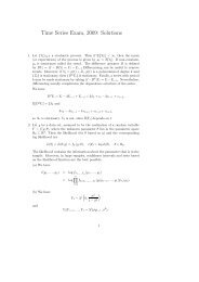
Time Series Exam, 2010: Solutions - STAT

Time Series Exam, 2010: Solutions
1. The autocorrelation function (ACF) of a process Y t is defined as
ρ(s,t) =
γ(s,t)
√
γ(s,s)γ(t,t)
,
where
γ(s,t) = E[(Y s −E(Y s ))(Y t −E(Y t ))]
is the autocovariance function, provided the expectations exist.
A strictly stationary time series is one for which the probabilistic behavior of every collection
of values {Y t1 ,Y t2 ,...,Y tk } is identical to that of the time shifted set {Y t1+h,Y t2+h,...,Y tk +h}.
That is,
P{Y t1 ≤ c 1 ,...,Y tk ≤ c k } = Prob{Y t1+h ≤ c 1 ,...,Y tk +h ≤ c k }
for all k = 1,2,..., all time points t 1 ,t 2 ,...,t k , all numbers c 1 ,c 2 ,...,c k , and all time shifts
h = 0,±1,±2,....
A second-order stationary time series, Y t , is a finite variance process such that
(a) the mean value function, µ t = E(Y t ) is constant and does not depend on time t, and
(b) the covariance function, γ(s,t) = E[(Y s −µ s )(Y t −µ t )] depends on s and t only through their
difference |s−t|.
A common tool to remove trends is differencing. It allows to remove linear or polynomial trends,
but it usually complicates the dependence structure of the process.
(a) We have
Y t
= δ +Y t−1 +ε t
= 2δ +Y t−2 +ε t−1 +ε t
= ...
t∑
= tδ +Y 0 + ε k .
k=1
(b) We have
and
( )
t∑
µ t = E(Y t ) = E tδ +Y 0 + ε k = tδ
k=1
γ ( s,t) = cov(Y s ,Y t )
(
= cov
= cov
sδ +Y 0 +
s∑
ε k ,tδ +Y 0 +
k=1
Ñ é
min(s,t)
∑
min(s,t)
∑
ε k , ε k
k=1
= min(s,t)σ 2 .
k=1
)
t∑
ε k
k=1
1

(c) We have
ρ(t−1,t) =
=
γ(t−1,t)
√
γ(t−1,t−1)γ(t,t)
(t−1)σ 2
√
(t−1)σ2 tσ 2
=
…
t−1
−→ 1, as t → ∞.
t
This means two observations far apart are strongly correlated.
(d) We showed in (b) that µ t depends on t and γ(s,t), on min(s,t).
(e) Let us consider the differenced series Ỹt = Y t −Y t−1 = ε t +δ. We have then µ t = δ, which
does not depend on t and cov(Y s ,Y t ) = cov(ε s +δ,ε t +δ) = σ 2 δ(s−t), where δ(s−t) = 1 if
s = t and 0 otherwise.
2. (a) See Lemma 18.
(b) Conditional on A = {Y t−r ,...,Y t−1 }, we find that E(Y t | A) = φy t−1 and E(Y t−r−1 | A) =
φ −1 y t−r , the latter because we can write Y t−r−1 = φ −1 (Y t−r −ε t−r ). Moreover,
E(Y t Y t−r−1 | A) = E{(φY t−1 +ε t )φ −1 (Y t−r −ε t−r ) | A} = y t−1 y t−r , r ≥ 1,
so the conditional covariance cov(Y t ,Y t−r−1 | A) = E(Y t Y t−r−1 | A)−E(Y t | A)E(Y t−r−1 | A) = 0.
If we see a series in which the partial autocorrelation function has zeros after a certain point, then
we use this property to diagnose an AR model, whereas the same property for the ACF suggests
an MA model. See slide 154 and previous material.
(c) The plots show the correlogram (empirical ACF) and partial correlogram empirical PACF)
for the data. The estimates on the left are moment-based, and those on the right are obtained
from them using the Yule–Walker equations. The horizontal dashed lines show significance limits
for the correlogram and partial correlogram elements, based on assumptions of white noise with
finite fourth moments; the limits are at ±2/ √ n.
The correlogramshows geometric decline with alternating sign, and suggests that this is an AR(1)
model with φ ≈ −0.9. This is confirmed by the PACF, which has just one significant value, at
h = 1, with value around −0.9.
3. If {γ h } h∈Z is the ACF of a stationary random sequence, then there exists a unique function F
defined on [−1/2,1/2] such that F(−1/2) = 0, F is right-continuous and non-decreasing, with
symmetric increments about zero, and
∫
γ h = e 2πihu dF(u), h ∈ Z.
(−1/2,1/2]
The function F is called the spectral distribution function of γ h , and its derivative f, if it exists,
is called the spectral density function. If ∑ h|γ h | < ∞, then f exists. A function f(ω) defined on
[−1/2,1/2] is the spectrum of a stationary process if and only if f(ω) = f(−ω), f(ω) ≥ 0, and
∫
f(ω)dω < ∞.
We have
γ(h) = E[(Y t+h −E[Y t+h ])(Y t −E[Y t ])]
[ ]
∑
= E ψ j ε t+h−j ·∑
ψ l ε t−l
j
= ∑ j
ψ j ψ j−h σ 2 ,
l
2

hence,
f(ω) = ∑ h
γ(h)e −2πωh
= σ 2∑ h
= σ 2∑ j
∑
ψ j ψ j−h e −2πiωj e 2πiω(j−h)
j
ψ j e −2πiωj∑ ψ k e 2πiωk
k
= σ 2 |ψ(ω)| 2 .
In the case of an ARMA(1,1) process (1−φB)Y t = (1+θB)ε t , we have
|φ(ω| 2 f Y (ω) = |θ(ω)| 2 f ε (ω).
We also have
and
|φ(ω| 2 = (1−φ 1 e −2πiω )(1−φ 1 e 2πiω )
|θ(ω)| 2 = (1+θ 1 e −2πiω )(1+θ 1 e 2πiω )
hence
f Y (ω) = σ 2|θ(ω)|2
|φ(ω)| 2
= σ 2 (1+θ 1e −2πiω )(1+θ 1 e 2πiω )
(1−φ 1 e −2πiω )(1−φ 1 e 2πiω )
= 1+2θ 2cos(2πiω)+θ1
2
1−2φ 1 cos(2πiω)+φ 2 .
1
4. A time series {Y t } is an autoregressive-moving average process of order p,q, ARMA(p,q), model,
if it is stationary and of the form
Y t = φ 1 Y t−1 +φ 2 Y t−2 +···+φ p Y t−p +ε t +θ 1 ε t−1 +···+θ q ε t−q ,
where φ 1 ,...,φ p ,θ 1 ,...,θ q are constants with φ p ,θ q ≠ 0, and v t is white noise.
An ARMA(p,q) process φ(B)Y t = θ(B)ε t is causal if it can be written as a linear process
Y t =
∞∑
ψ j ε t−j = ψ(B)ε t ,
where ∑ |ψ j | < ∞, and we set ψ 0 = 1. It is invertible if it can be written as
ε t =
where ∑ |π j | < ∞, and we set π 0 = 1.
j=0
∞∑
π j Y t−j = π(B)Y t ,
j=0
An ARMA(p,q) process φ(B)Y t = θ(B)ε t is causal iff φ(z) ≠ 0 within the unit disk D. If so, then
the coefficients of ψ(z) satisfy ψ(z) = θ(z)/φ(z) for z ∈ D. The process is invertible iff θ(z) ≠ 0
for for z ∈ D. If so, then the coefficients of π(z) satisfy π(z) = φ(z)/θ(z) for for z ∈ D.
(a) Since 1−0.8x+0.15x 2 = (1−0.3x)(1−0.5x), we get
Y t = ε t −0.5ε t−1
and so this is a causal and invertible MA(1) process (φ(z) = 1 and θ(z) = 1−0.3z has root
1/0.3). We have
γ(h) = 1.25σ 2 δ(h)−0.5σ 2 (δ(h+1)+δ(h−1))
so except ρ 0 = 1, we’ll only have ρ 1 = −0.4.
3

(b) Since the roots of 1 −x+0−5x 2 are (1±i)/2, this is an ARMA(2,1) process. Moreover,
it is neither causal nor invertible since the two roots of φ(z) lie inside the unit disk and the
root of θ(z) is 1.
(c) Here, we have
γ(h) = 5σ 2 δ(h)−2σ 2 (δ(h+1)+δ(h−1))
and so we have the same ACF as we had in (a). The two processes are the same (provided
the variance of the white noise is such that the two autocovariance functions are identical),
but the model in (a) is invertible, whereas the model in (c) is not.
5. See the notes.
6. All linear state space models involve two equations, the state equation, which determines the
evolution of an underlying unobserved state, and the observation equation, which determines how
the observed data are related to the state. The local trend model (a simple special case) has
State equation:
Observation equation:
µ t+1 = µ t +η t , η t
iid
∼ N(0,σ
2
η ),
y t = µ t +ε t , ε t
iid
∼ N(0,σ 2 ),
where the η t and ε t are mutually independent. We suppose that data y 1 ,...,y n are available.
Let H t denote the information available at time t. Filtering is the estimation of µ t using H t ,
smoothing is the estimation of µ t using H n and prediction is the forecasting µ t+h fot h > 0 using
H t .
(a) We have
State equation:
Observation equation:
X t = −0.9X t−2 +ε t , ε t
iid
∼ N(0,σ
2
ε ),
Y t = X t +η t , η t
iid
∼ N(0,σ
2
η ).
(b) Since η t is an independent white noise, Y t is stationary if and only if X t is stationary.
Moreover, X t is an AR(2) model, so provided the variances σ0 2 and σ2 1 are such that var(X t)
does not depend on t, Y t is stationary. Since
®
(−0.9) t/2 X
X t = 0 + ∑ t/2
k=1 ε 2k(−0.9) t/2−k , t even,
(−0.9) (t+1)/2 X −1 + ∑ (t−1)/2
k=0
ε 2k+1 (−0.9) (t−1)/2−k , t odd,
the variance of X t is given by
{
var(X t ) =
σ0 2(−0.9)t +σε
2 1−(0.81) t/2
1−0.81
, t even,
σ1 2(−0.9)t+1 +σε
2 1−(0.81) (t+1)/2
1−0.81
, t odd,
and so X t and Y t are stationary if and only if
σ 2 0 = σ2 1 =
σ 2 ε
1−0.81 .
(c) The left time plot (X t ) shows clearly the AR(2) structure, whereas on the right time plot, it
is more difficult to see, because of the noise η t . The range is also more important (from -10
to 5 instead of -8 to 2). The left ACF is typical from an AR(2) model with such parameters.
On the right one, the added noise reduces the proportion of information in the observation
and the correlation, so the values are diminished on the plot. Finally, on the left PACF, we
clearly find the model structure, whereas on the right one, we also have the consequences of
the added noise.
4