Monte Carlo Inference - STAT - EPFL

Monte Carlo InferenceAnthony Davisonc○2009http://stat.epfl.chVariable dimension MCMC 193Motivation . . . . . . . . . . . . . . . . . . . . . . . . . . . . . . . . . . . . . . . . . . . . . . . . . . . . . . . . . . . 194Galaxy data . . . . . . . . . . . . . . . . . . . . . . . . . . . . . . . . . . . . . . . . . . . . . . . . . . . . . . . . . . 195Cyclones data. . . . . . . . . . . . . . . . . . . . . . . . . . . . . . . . . . . . . . . . . . . . . . . . . . . . . . . . . 199Dimension-matching moves. . . . . . . . . . . . . . . . . . . . . . . . . . . . . . . . . . . . . . . . . . . . . . . . 202Acceptance probability . . . . . . . . . . . . . . . . . . . . . . . . . . . . . . . . . . . . . . . . . . . . . . . . . . . 203Comments . . . . . . . . . . . . . . . . . . . . . . . . . . . . . . . . . . . . . . . . . . . . . . . . . . . . . . . . . . . 204Poisson process with changepoints. . . . . . . . . . . . . . . . . . . . . . . . . . . . . . . . . . . . . . . . . . . 205Heights of steps . . . . . . . . . . . . . . . . . . . . . . . . . . . . . . . . . . . . . . . . . . . . . . . . . . . . . . . 206Locations of steps . . . . . . . . . . . . . . . . . . . . . . . . . . . . . . . . . . . . . . . . . . . . . . . . . . . . . . 207Updating . . . . . . . . . . . . . . . . . . . . . . . . . . . . . . . . . . . . . . . . . . . . . . . . . . . . . . . . . . . . 208Birth. . . . . . . . . . . . . . . . . . . . . . . . . . . . . . . . . . . . . . . . . . . . . . . . . . . . . . . . . . . . . . . 209Algorithm . . . . . . . . . . . . . . . . . . . . . . . . . . . . . . . . . . . . . . . . . . . . . . . . . . . . . . . . . . . 212Output . . . . . . . . . . . . . . . . . . . . . . . . . . . . . . . . . . . . . . . . . . . . . . . . . . . . . . . . . . . . . 213Discussion . . . . . . . . . . . . . . . . . . . . . . . . . . . . . . . . . . . . . . . . . . . . . . . . . . . . . . . . . . . 2151

Week 10Variable dimension MCMCMonte Carlo Inference Spring 2009 – slide 192Variable dimension MCMC slide 193Motivation□ Many important statistical models of scientific interest are such thatThe number of things you do not know is one of the things you do not know.(Green, 1995)□ Examples are:– mixture models with an unknown number of components– changepoint models with an unknown number of changepoints– Bayesian model comparison problems□ In this case an MCMC algorithm needs to be able to jump between parameter spaces of differentdimensions, and special algorithms are needed□ The standard approach is the reversible jump Markov chain Monte Carlo algorithm, whichgeneralises the Metropolis–Hastings algorithm□ Goal today is to sketch such algorithms by looking in detail at an example.Monte Carlo Inference Spring 2009 – slide 194Example: Galaxy dataVelocities (km/second) of 82 galaxies in a survey of the Corona Borealis region. The error is thoughtto be less than 50 km/second.9172 9350 9483 9558 9775 10227 10406 16084 16170 1841918552 18600 18927 19052 19070 19330 19343 19349 19440 1947319529 19541 19547 19663 19846 19856 19863 19914 19918 1997319989 20166 20175 20179 20196 20215 20221 20415 20629 2079520821 20846 20875 20986 21137 21492 21701 21814 21921 2196022185 22209 22242 22249 22314 22374 22495 22746 22747 2288822914 23206 23241 23263 23484 23538 23542 23666 23706 2371124129 24285 24289 24366 24717 24990 25633 26960 26995 3206532789 34279Monte Carlo Inference Spring 2009 – slide 195196

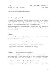
Galaxy dataSpeed10 15 20 25 30 35Normal Q−Q Plot−2 −1 0 1 2Theoretical QuantilesMonte Carlo Inference Spring 2009 – slide 196Mixture density□ Natural model for such data is a p-component mixture densityf(y;θ) =p∑π r f r (y;θ), 0 ≤ π r ≤ 1,r=1p∑π r = 1,where π r is the probability that Y comes from the rth component and f r (y;θ) is its densityconditional on this event.□ Widely used class of models, often with number of components p unknown.□ Aside: such models are non-regular for some likelihood inferences:– non-identifiable under permutation of components;– setting π r = 0 eliminates parameters of f r ;– maximum of likelihood can be +∞, achieved for several θMonte Carlo Inference Spring 2009 – slide 197r=1197

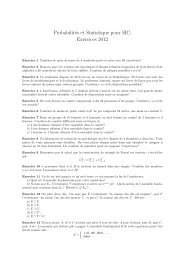
How many components?p 1 2 3 4 5Parameters 2 5 8 11 14̂l −240.42 −220.19 −203.48 −202.52 −192.42Fitted mixture model with p = 4 normal components:PDF0.0 0.05 0.10 0.15 0.200 10 20 30 40VelocityMonte Carlo Inference Spring 2009 – slide 198Cyclones dataTimes of major cyclonic storms striking the Bay of Bengal from 1877–1977.Cumulative number of storms0 20 40 60 80 100 120 1401880 1900 1920 1940 1960 1980Time (years)How many changepoints?Monte Carlo Inference Spring 2009 – slide 199198

Dimension-matching moves□ We want to compute the probability of jumping from point u (1) ∈ R n 1to u (2) ∈ R n 2, wheren 1 ≠ n 2 . To do so, we introduce– auxiliary variables w 1 ∈ R m 1, w 2 ∈ R m 2, whose dimensions are chosen so thatn 1 + m 1 = n 2 + m 2– a random variable t which gives a bijection between (u (1) ,w 1 ) ↔ (u (2) ,w 2 ),t = t 1 (u (1) ,w 1 ) = t 2 (u (2) ,w 2 ) ∈ R n 1+m 1□ Then the probability π(u)q(v | u) is replaced byπ{(1,u (1) ) | y} × q(1,u (1) ∂(u (1) ,w 1 )) × p 1 (w 1 ) ×∣ ∂t ∣where the terms are– the posterior probability of being at u (1) in R n 1– the probability of proposing a move away from this point– the density of w 1– the Jacobian transforming the preceding terms into a density for tMonte Carlo Inference Spring 2009 – slide 202Acceptance probability□ The probability π(v)q(u | v) is likewise replaced byπ{(2,u (2) ) | y} × q(2,u (2) ∂(u (2) ,w 2 )) × p 2 (w 2 ) ×∣ ∂t ∣so the acceptance probability ratio π(v)q(u | v)/{π(u)q(v | u)} for the proposed move from(u (1) ,w 1 ) ↦→ (u (2) ,w 2 ) isπ{(2,u (2) ) | y}q(2,u (2) )p 2 (w 2 )∂(u (2) ,w 2 )π{(1,u (1) ) | y}q(1,u (1) )p 1 (w 1 ) ∣∂(u (1) ,w 1 ) ∣□ Often in practice the moves are set up so that m 1 = 0 or m 2 = 0, in which case there is no needto generate w 1 or w 2 . For example, if m 2 = 0, then the acceptance probability for theMetropolis–Hastings step ismin{1,where w ≡ w 1 .π{(2,u (2) ) | y}q(2,u (2) )π{(1,u (1) ) | y}q(1,u (1) )p 1 (w)}∂(u (2) )∣∂(u (1) , (10),w) ∣Monte Carlo Inference Spring 2009 – slide 203200

Heights of steps□ Conditional on k, u 1 ,... ,u k , we suppose that the heights satisfyλ 0 ,... ,λ k | u 1 ,... ,u k ,kiid ∼Γ(α,β)β ∼ Γ(e,f)α ∼ Γ(c,d),with c,d,e,f determined in advance (below we take e = f = 1, c = d = 2).□ This hierarchical model givesindλ j | rest ∼ Γ(α + n j ,β + u j+1 − u j ), j = 0,... ,k,⎧⎫⎨k∑ ⎬β | rest ∼ Γ⎩ e + (k + 1)α,f + λ j⎭j=0⎛ ⎞α c−1αk∏π(α | rest) ∝ ⎝e −dΓ(α) k+1 β k+1 ⎠ ,j=0□ Gibbs updates are possible for λ 0 ,...,λ k and β, and a random walk Metropolis step can be usedto update α, setting log α ′ ∼ N(log α,σ 2 ) (with σ = 0.5 below)Monte Carlo Inference Spring 2009 – slide 206Locations of steps□ To update the step locations u 1 ,... ,u k , we note that the joint density of the even order statisticsu 1 < · · · < u k from a random sample of size 2k + 1 from the U(0,L) distribution is(2k + 1)!L 2k+1 u 1 (u 2 − u 1 ) · · · (u k − u k−1 )(u k+1 − u k ),used to discourage changepoints from occurring too close together.□ We choose j ′ ∈ {1,... ,k} uniformly at random, and then propose to replace u j withu ′ j ∼ U(u j−1,u j+1 ), with the acceptance probability beingwhere L is the likelihood ratio{min 1,L × (u′ j − u j−1)(u j+1 − u ′ j ) }(u j − u j−1 )(u j+1 − u j )L = λn′ j−1j−1 e−λ j−1(u ′ j −u j−1) λ n′ jj e−λ j(u j+1 −u ′ j )λ n j−1j−1 e−λ j−1(u j −u j−1 ) λ n jj e−λ j(u j+1 −u j )and n ′ j−1 and n′ j are the numbers of events in the proposed new intervals [u j−1,u ′ j ) and[u ′ j ,u j+1).Monte Carlo Inference Spring 2009 – slide 207202

UpdatingWe can now update the parameters λ 0 ,... ,λ k , u 1 ,... ,u k , β, α, giving posterior realisations of λ(u)like those below, for k = 0,1,2,3:Intensity0 1 2 3 4 5Intensity0 1 2 3 4 51880 1900 1920 1940 1960 19801880 1900 1920 1940 1960 1980Intensity0 1 2 3 4 5Intensity0 1 2 3 4 51880 1900 1920 1940 1960 19801880 1900 1920 1940 1960 1980Monte Carlo Inference Spring 2009 – slide 208Birth□ For the birth move, we first must propose a new location u ∗ , which will lie in the interval(u j ,u j+1 ), for j ∈ {0,... ,k}, and new heights for the corresponding interval.□ We take u ∗ ∼ U(0,L), and let λ ′ j ,λ′ j+1 denote the new heights, defined through(u j+1 − u ∗ )log λ ′ j+1 + (u∗ − u j )log λ ′ j = (u j+1 − u j )log λ j ,where w ∼ U(0,1). With a = (u ∗ − u j )/(u j+1 − u j ) this givesλ ′ j+1λ ′ j= 1 − ww ,λ j = (λ ′ j )a (λ ′ j+1 )1−a , w =λ ′ jλ ′ j + λ′ j+1and ensures that λ j lies between the proposed new heights.□ If the move is accepted we must set k ↦→ k + 1, relabel the new positionsu 1 ,... ,u j ,u ∗ ,u j+1 ,...,u k and the new heights λ 1 ,...,λ ′ j−1 ,λ′ j ,... ,λ k.□ We write the probability of acceptance asmin {1,(likelihood ratio) × (prior ratio) × (proposal ratio) × (Jacobian)}□ We put a prior distribution p j = Pr(k = j) on the number of steps j ∈ {0,... ,k max }.Monte Carlo Inference Spring 2009 – slide 209203

Birth□ We find thatlikelihood ratio =λ′ n ′j−1je −λ′ j (u∗ −u j ) × λ ′ j+1n ′ j+1e −λ′ j+1 (u j+1−u ∗ )λ n jj e−λ j(u j+1 −u j )prior ratio = p k+1 (2k + 3)(2k + 2) (u j+1 − u ∗ )(u ∗ − u j )p k L 2 (u j+1 − u j )× βαΓ(α)( λ′j λ ′ j+1λ j) α−1exp { −β(λ ′ j + λ ′ j+1 − λ j ) } ,proposal ratio = d k+1/(k + 1),b k /L∂(λJacobian =′ j ,λ′ j+1 )∣ ∂(λ j ,w) ∣ = (λ′ j + λ′ j+1 )2,λ j□ The proposal ratio for the birth move is the ratio of the probability for the corresponding death(k + 1) ↦→ k (which chooses one of the steps to remove at random) to the birth move (choosing arandom site for u ∗ )□ The Jacobian is obtained from the mapping (λ j ,w) ↦→ (λ ′ j ,λ′ j+1 ) on the previous slide. In termsof the general discussion leading to (10) we have u (1) ≡ λ j , u (2) ≡ (λ ′ j ,λ′ j+1 ).Monte Carlo Inference Spring 2009 – slide 210,Death□ The death move (k + 1) ↦→ k has to correspond to the birth move, so we sample a changepointj ∈ {1,... ,k + 1} at random, with probability (k + 1) −1 , and try to merge the values of λ j−1 , λ jto get λ ′ j−1 using the formula(u j+1 − u j )log λ j + (u j − u j−1 )log λ j−1 = (u j+1 − u j−1 )log λ ′ j−1 ,to correspond to the birth move.□ If the death move is accepted, then u 1 ,... ,u k+1 and λ 0 ,...,λ k+1 are modified by dropping u jand mapping (λ j ,λ j+1 ) ↦→ λ ′ j , with k ↦→ k − 1 and changepoints correspondingly relabelled.□ The acceptance probability for the death move (k + 1) ↦→ k is{}1min 1,(likelihood ratio) × (prior ratio) × (proposal ratio) × (Jacobian)where the terms here are those given on the previous slide for the birth move k ↦→ (k + 1), withonly minor notational changes to account for the fact that the inverse move is being proposed.Monte Carlo Inference Spring 2009 – slide 211204

Algorithm□ At each iteration the MCMC code then amounts to– attempt a birth move with probability b k– attempt a death move with probability d k– attempt an update move with probability 1 − b k − d kuntil finished.□ Coded in R (around 10 hours), 10 5 steps took around 60 seconds□ The code is a little complex, because– in R arrays cannot start with index 0, so care is needed with subscripts– the state vector is (k,β,α,λ 0 ,...,λ k ,u 1 ,... ,u k ), of length 2k + 4, which keeps changing. socare is needed to ensure the right parameters are used at each step□ Specialised convergence diagnostics are needed, because the meaning of the parameters changes:for example λ 4 only exists when k ≥ 4.Monte Carlo Inference Spring 2009 – slide 212OutputLeft: 20 realisations from the reversible jump chain. Right: average rate λ(u) from the 10 5 realisationsIntensity0 1 2 3 4 5Mean intensity0 1 2 3 4 51880 1920 19601880 1920 1960Monte Carlo Inference Spring 2009 – slide 213205

OutputPrior (black) and posterior (red) distributions of the number of changepoints; the prior is Poisson withmean 3, truncated to {0,1,... ,12}Density0.00 0.05 0.10 0.15 0.20 0.25 0.300 2 4 6 8 10 12kMonte Carlo Inference Spring 2009 – slide 214Discussion□ Many more quantities could be extracted from the output, such as– positions of changepoints, conditional on different values of k– heights of steps, conditional on different values of k– uncertainties for posterior mean/median of λ(u)□ RJMCMC algorithms are increasingly widely used for complex problems□ Pluses:– they provide a way to allow for model uncertainty as k varies– powerful generalisation of the Metropolis–Hastings algorithm□ Minuses:– can be difficult to invent good proposals (with high probabilities of acceptance) for thebirth/death moves– programming them is time-consuming and fiddleyMonte Carlo Inference Spring 2009 – slide 215206