Statistics I Exercises

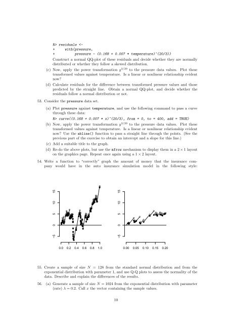
R> residuals curve((0.168 + 0.007 * x)^(20/3), from = 0, to = 400, add = TRUE)(b) Now, apply the power transformation y 3/20 to the pressure data values. Plot thesetransformed values against temperature. Is a linear or nonlinear relationship evidentnow? Use the abline() function to pass a straight line through the points. (See theprevious part of the exercise to obtain an intercept and a slope for this line.)(c) Add a suitable title to the graph.(d) Re-do the above plots, but use the mfrow mechanism to display them in a 2 × 1 layouton the graphics page. Repeat once again using a 1 × 2 layout.54. Write a function to “correctly” graph the amount of money that the insurance companywould have in the auto insurance simulation model in the following style:●−5 0 5 10 15● ●● ●●●●● ● ●●● ●●●● ● ● ● ● ●●●●● ●●● ● ● ●●●●● ●●● ●●● ● ●●●●●●● ●● ●●● ●● ●● ●●●●● ● ●●●● ●●● ●● ●● −5 0 5 10 15●●●●● ●● ●●●●● ●●●●●● ● ●● ● ●● ● ● ●●● ●●●●● ●●● ●● ●●0.0 0.2 0.4 0.6 0.8 1.00.00 0.05 0.10 0.15 0.2055. Create a sample of size N = 128 from the standard normal distribution and from theexponential distribution with parameter 1, and use Q-Q plots to assess the normality of thedata. Describe and explain the differences of the results.56. (a) Generate a sample of size N = 1024 from the exponential distribution with parameter(rate) λ = 0.2. Call x the vector containing the sample values.10