Automatic Exposure Correction of Consumer Photographs
Automatic Exposure Correction of Consumer Photographs
Automatic Exposure Correction of Consumer Photographs

Create successful ePaper yourself
Turn your PDF publications into a flip-book with our unique Google optimized e-Paper software.
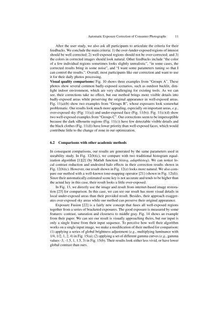
<strong>Automatic</strong> <strong>Exposure</strong> <strong>Correction</strong> <strong>of</strong> <strong>Consumer</strong> <strong>Photographs</strong> 11<br />
After the user study, we also ask all participants to articulate the criteria for their<br />
feedbacks. We conclude the main criteria: 1) the over-/under-exposed regions <strong>of</strong> interest<br />
should be well corrected; 2) well-exposed regions should not be over-corrected; and 3)<br />
the colors in corrected images should look natural. Other feedbacks include “the color<br />
<strong>of</strong> a few individual regions sometimes looks slightly unrealistic”, “in some cases, the<br />
corrected results bring in some noise”, and “I want some parameters tuning so that I<br />
can control the results.”. Overall, most participants like our correction and want to use<br />
it for their daily photos processing.<br />
Visual quality comparisons: Fig. 10 shows three examples from “Groups A”. These<br />
photos show several common badly-exposed scenarios, such as outdoor backlit, dimlight<br />
indoor environment, which are very challenging for existing tools. As we can<br />
see, their corrections take no effect, but our method brings more visible details into<br />
badly-exposed areas while preserving the original appearance in well-exposed areas.<br />
Fig. 11(a)(b) show two examples from “Groups B”, whose exposures look somewhat<br />
problematic. Our results look much more appealing, especially on important areas, e.g.,<br />
over-exposed sky (Fig. 11(a)) and under-exposed face (Fig. 11(b)). Fig. 11(c)(d) show<br />
two well-exposed examples from “Groups C”. Our corrections seem to be imperceptible<br />
because the dark silhouette regions (Fig. 11(c)) have few detectable visible details and<br />
the black clothes (Fig. 11(d)) have lower priority than well-exposed faces, which would<br />
contribute little to the change <strong>of</strong> zone in our optimization.<br />
6.2 Comparisons with other academic methods<br />
In consequent comparisons, our results are generated by the same parameters used in<br />
useability study. In Fig. 12(b)(c), we compare with two traditional histogram equalization<br />
algorithm [1][2] (by Matlab function histeq, adapthisteq). We can notice local<br />
contrast reduction and undesired halo effects in their correction results shown in<br />
Fig. 12(b)(c). However, our result shown in Fig. 12(e) looks more natural. We also compare<br />
our method with a well-known tone-mapping operator [21] (shown in Fig. 12(d)).<br />
Since their automatically estimated scene key is not accurate and tends to be higher than<br />
the actual key in this case, their result looks a little over-exposed.<br />
In Fig. 13, we directly use the image and result from internet-based image restoration<br />
[23] for comparison. In this case, we can see our result has more visual details in<br />
local under-exposed areas than their provided result. Besides, their approach exaggerates<br />
over-exposed sky areas while our method can preserve their original appearance.<br />
<strong>Exposure</strong> Fusion [22] is a fairly new concept that fuses all well-exposed regions<br />
together from a series <strong>of</strong> bracketed exposures. The good exposure is measured by some<br />
features: contrast, saturation and closeness to middle gray. Fig. 14 shows an example<br />
from their paper. We can see our result is visually approaching theirs, but our input is<br />
only a single frame from their input sequence. To perceive how well their algorithm<br />
works on a single input image, we make a modification <strong>of</strong> their method for comparison:<br />
(1) applying a series <strong>of</strong> global brightness adjustment (e.g., multiplying luminance with<br />
1/4, 1/2, 1, 2, 4) in Fig. 15(a); (2) applying a set <strong>of</strong> different gamma curves (e.g., gamma<br />
values -3, -1.5, 1, 1.5, 3) in Fig. 15(b). Their results look either less vivid, or have lower<br />
global contrast than ours.