Automatic Exposure Correction of Consumer Photographs

More documents

Recommendations

Info

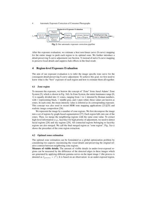
4 Automatic Exposure Correction of Consumer Photographs I in Auto-level Stretch Region Segmentation High-level features Region-level Exposure Evaluation Region Analysis Estimate Optimal Zone of Region Fig. 2. Our automatic exposure correction pipeline Detail-preserving S-curve Adjustment After the exposure evaluation, we estimate a best non-linear curve (S-curve) mapping for the entire image to push each region to its optimal zone. We further introduce a detail-preserving S-curve adjustment (see Section 5) instead of naïve S-curve mapping to preserve local details and suppress halo effects in the final result. 4 Region-level Exposure Evaluation The aim of our exposure evaluation is to infer the image specific tone curve for the consequent detail-preserving S-curve adjustment. To achieve this goal, we first need to know what is the “best” exposure of each region and how to estimate them all together. 4.1 Zone region To measure the exposure, we borrow the concept of “Zone” from Ansel Adams’ Zone System [5], which is shown in Fig. 3(d). In Zone System, the entire luminance range [0, 1] is equally divided into 11 zones, ranging from O to X denoted by Roman numbers, with O representing black, V middle gray, and X pure white; these values are known as zones. In each zone, the mean intensity value is referred as its corresponding exposure. This concept was also used in recent HDR tone mapping applications [21][25] and realistic image composition [26]. We represent the image by a number of zone regions. We first decompose the image into a set of regions by graph-based segmentation [27]. Each region falls into one of the zones. Then, we merge the neighboring regions with the same zone value. To extract high-level information (e.g., face/sky) for high priority of adjustment, we need to detect facial regions [28] and sky regions [29]. All connected regions belonging to face/sky regions are also merged. We call the final merged region as “zone region”. Fig. 3(a-c) shows the procedure of the zone region extraction. 4.2 Optimal zones estimation The optimal zone estimation can be formulated as a global optimization problem by considering two aspects: maximizing the visual details and preserving the original relative contrast between neighboring zone regions. Measure of visible details. The amount of visible details in under-/over-exposed regions can be measured by the difference of the detected edges in these images which are generated by applying different gamma-curves on the input image I (the process is denoted as Igamma = I γ ). It is based on an observation: in an under-exposed region, I out
Automatic Exposure Correction of Consumer Photographs 5 Zone VIII Zone VII Zone IV Zone III Zone II Zone I Zone O (a) input image (b) segmented regions [10] (c) initial zones of grouped regions z e : O I II III IV V VI VII VIII IX X : 0 0.1 0.2 0.3 0.4 0.5 0.6 0.7 0.8 0.9 1.0 (d) Ansell Adam’s zones z (Roman numeral) and corresponding exposures e (decimal number) Fig. 3. Zone region extraction. In (c), different colors denote different zone regions, in which the Roman numbers denote corresponding zone values. s h all (a) input luminance channel (b) visible shadow edges Ω (c) visible highlight edges Ω (d) all visible edges Ω Fig. 4. Measure of visible details. In (b-d), white lines are detected edges by Canny operator. Ri Fig. 5. Relative contrast dij is the histogram distance between two neighboring regions Ri, Rj. dij we can detect more/less visible edges after the gamma correction when the gamma γ is smaller/larger, and the edge number difference between two gamma-corrected images (one with small gamma, the other with large gamma) indicates the amount of recoverable details. The similar process can be applied to the over-exposed region as well. In our implementation, we use two default gamma values γ = 2.2 and γ−1 = 0.455. We first detect edges on three images I, Iγ , Iγ−1 by the same Canny operator [1] to obtain three edge sets: Ω1, Ωγ, Ωγ−1. The visible details in the shadow region (zone value < V) and the highlight region (zone value > V) are measured by: Ωs = Ωγ−1 � − Ωγ−1 Ωγ and Ωh � = Ωγ − Ωγ−1 Ωγ, shown in Fig. 4 (b)(c). Note that the absolute differences Ω s and Ω h cannot be directly used since they vary from image to image. To obtain a comparable measure, we compute the relative visibility of details: ν s = |Ω s | �� all Ω � � � h , ν = �Ωh � � �� all Ω � � (1) where | · | indicates the edge number in a set, and Ωall � � = Ω1 Ωγ Ωγ−1 is the union of all three sets, shown in Fig. 4 (d). Measure of relative contrast. We measure the relative contrast between zone regions using their intensity histogram distance. This distance is defined as the minimum shifting distance of two histograms to maximize their intersection (shown in Fig. 5). We use Rj
Page 1 and 2: Automatic Exposure Correction of Co
Page 3: 2 Related Work Automatic Exposure C
Page 7 and 8: output intensity 1 0.9 0.8 0.7 0.4
Page 9 and 10: 6 Experiments 6.1 Usability Study A
Page 11: Automatic Exposure Correction of Co
Page 14: 14 Automatic Exposure Correction of

Automatic Exposure Correction of Consumer Photographs

Create successful ePaper yourself

Delete template?

Save as template?