Automatic Exposure Correction of Consumer Photographs

8 Automatic Exposure Correction of Consumer Photographs
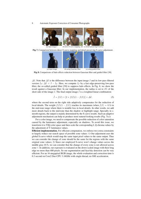
(a) input image I (b) naive S-curve mapping f(I) (c) detail-preserving S-curve
Î
Fig. 7. Comparison between direct S-curve mapping and detail-preserving S-curve adjustment.
(a) input image (b) using Gaussian filter (c) using guided filter
Fig. 8. Comparisons of halo effects reduction between Gaussian filter and guided filter [30].
∆I. Note that ∆I is the difference between the input image I and its low-pass filtered
version IF : ∆I = I − IF . Here, we compute IF by a fast edge-preserving low-pass
filter, the so-called guided filter [30] to suppress halo effects. In Fig. 8, we show the
result against a Gaussian filter. In our implementation, the radius is set to 4% of the
short side of the image I. The final output image Î is a weighted linear combination:
Î = f(I) + [2 × f(I)(1 − f(I))] × ∆I, (5)
where the second term on the right side adaptively compensates for the reduction of
local details. The weight f(I)(1 − f(I)) reaches its maximum (when f(I) = 0.5) in
the mid-tone range where there is notable loss in local details. In other words, we add
more details back to the mid-tone than the shadow or highlight range. Specially in smooth
regions, the output is mainly determined by the S-curve results. Such an adaptive
adjustment mechanism can help us produce more natural-looking results (Fig. 7(c))
For a color image, we need to compensate the possible reduction of color saturation
caused by the luminance adjustment, especially on shadows. To avoid this issue, we
transform it to YIQ color space and then scale the corresponding I, Q chroma values by
the adjustment of Y luminance values.
Efficient implementation. For efficient computation, we enforce two extra constraints
to largely reduce our search space of possible zone values: 1) Our adjustment uses the
global S-curve which would map the same input pixel values to the same output. Thus
we can consider the change of zone should be the same for the regions with the same
original zone values; 2) Since our employed S-curve won’t change values across the
middle gray (0.5), we can consider that the change of every zone is not allowed across
zone V. In addition, our exposure is evaluated on the down-scaled image with their long
edge no more than 400 pixels. So our segmentation and face/sky detection can be very
efficient. For an 16-megapixel RGB image, the whole evaluation and correction time is
0.3 second on Core2 Duo CPU 3.16GHz with single-thread, no SSE acceleration.