Automatic Exposure Correction of Consumer Photographs

output intensity
1
0.9
0.8
0.7
0.4
0.3
0.2
0.1
Automatic Exposure Correction of Consumer Photographs 7
(a)
0.6
0.5
(b)
s
0
0 0.1 0.2 0.3 0.4 0.5 0.6 0.7 0.8 0.9 1
input intensity
h
output intensity
0.5
0.4
0.3
0.2
0.1
amount : 100%
amount : 60%
amount : 30%
0
0 0.1 0.2 0.3 0.4 0.5 0.6 0.7 0.8 0.9 1
input intensity
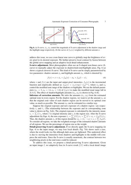
Fig. 6. (a) S-curve, φs, φh control the magnitude of S-curve adjustment in the shadow range and
the highlight range respectively. (b) the curves of f∆(x) weighted by different amount φ.
address this issue, we use a non-linear tone curve to globally map the brightness of every
pixel to its desired exposure. We further preserve local contrast by fusion between
the global curve mapping and an adaptive local detail enhancement.
S-curve adjustment. Most photographers often use an S-shaped non-linear curve (Scurve)
to manually adjust the exposure in shadow/mid-tone/highlight areas. Fig. 6 (a)
shows a typical (inverse) S-curve. This kind of S-curve can be simply parameterized by
two parameters: shadow amount φs and highlight amount φh, which is denoted by:
f(x) = x + φs × f∆(x) − φh × f∆(1 − x), (4)
where x and f(x) are the input and output pixel intensities. f∆(x) is the incremental
function and empirically defined as: f∆(x) = κ1x exp (−κ2x κ3 ), where κ2 and κ3
control the modified tone range of the shadows or highlights. We use the default parameters
(κ1 = 5, κ2 = 14, κ3 = 1.6) of f∆(x) to make the modified tonal range fall in
[0, 0.5]. The effect of shadow/highlight amounts (φs, φh) is shown in Fig. 6 (b).
Inference of correction amounts. We infer the amounts (φs, φh) from the estimated
optimal zone in every region. For the shadow regions, we want to set the amount φs so
that the original zone value of each shadow region can be moved to its optimal zone
value, as much as possible. The amount φh can be estimated in a similar way.
Suppose the original exposure and new exposure of a shadow region i are respectively
ei and êi. (The relationship between the exposure and its corresponding zone
value is shown on Fig. 3(d)). The original exposure is calculated by the intensity mean:
ei = � I/ci, where I is original intensity and ci is the region size. After the S-curve
adjustment (by Eqn. 4), the new exposure êi = � f(I)/ci = � (I + φs × f∆(I))/ci.
Thus, the shadow amount φs of this region should be: φs = (êi − ei) × ci × � f∆(I).
To consider all regions, we take the weighted average of the estimated shadow amounts
of all regions. We use the percentage of region size as the weight.
Detail-preserving S-curve adjustment. If we directly apply the S-curve mapping (in
Eqn. 4) to the input image, we may lose local details. Fig. 7(b) shows such a case,
where the result looks too flat although dark areas are lightened. This undesired effect
is due to: moving the intensities from shadows and highlights to the middle will compress
the mid-tones. Since the S-curve is usually monotonic, the contrast between two
neighboring pixels in the mid-tones could be reduced.
To address this issue, we propose a detail-preserving S-curve adjustment. Given
an input image I, we adaptively fuse its S-curve result f(I) with a local detail image