System Modelling: from DFA to Coloured Petri Nets - MegaByte

System Modelling: from DFA to Coloured Petri NetsDragan Mihaita, Ing. Sis. Drd., University of BucharestABSTRACTIn this paper we present some advantages and disadvantages offered by the classical theory of Petri Netstogether with a generalized class, Coloured Petri Nets used in modeling and simulation of the systems.Because by modeling and simulation can be obtained valuable information on real systems, informationswhich bring about major contributions to the development and enhancement of these systems, and knowing newways of modeling and simulation can be made comparative tests which provide results much close to the evolutionof systems real.Thus, starting with the modelling from a finite state machine and using the facilities offered by Petri NetsLocation / Transition together with their extensions, we demonstrate the usefulness of using Coloured Petri Nets inthe modeling and simulation of the systems.Keywords: finite state machine, state, transition, action, deterministic finite state automaton, modeling, simulation,Petri Nets location / transition, Coloured Petri Nets.1 INTRODUCTIONThere are subclasses of the class Petri Nets Location / Transition such as : Machine State, Graphs oftiming, Petri Nets with Free Choice, Petri Nets with Free Choice Extended, Petri Nets Simple which have the samepower of modeling with Deterministic Finite Automata. To the systems (phenomena) that can not be modeled byPetri Nets Location/Transition classes appeared the need for extend this class, which leaded at obtaining newclasses of Petri Nets:‣ Petri Nets with Priorities, Petri Nets with Inhibitions, Petri Nets with Reset, Petri NetsControlled with Automatic, which having superior power of the modelling compared with Petri Nets Location /Transition.Was searched a unified theory of Petri nets by introducing a class in which are included Petri nets Location/ Trazitie and their extensions, the class with power by modeling upper all the classes previously introduced, whatleaded to obtain the class Coloured Petri Nets.2 PRELIMINARIESFor develop this paper we have needed of several definitions and theoretical results.Definition 2.1[6,7] Is called finite-state machine (FSM) or finite-state automaton (FA) or „machine with a finitenumber of states " a model of behavior composed of states, transitions and actions. Ie a finite state automaton is amathematical object form FA = (S, T, m, s 0 , F) where :‣ S is the finite set of states;‣ T is the finite set, called input alphabet;‣ m : S x (T {})P(S) is the partial function of the next state;‣ s 0 S is a state called state of starting or the initially state ;‣ F S is a set of state called the set of the final states ( of acceptance).In such a model:State is determined by past states of the system. As such, it can be said to record information about thepast, i.e., it reflects the input changes from the system start to the present moment.Transition indicates a state change and is described by a condition that would need to be fulfilled to enablethe transition..Action is a description of an activity that is to be performed at a given momen.There are several types of actions, such as : Entry action which is performed when entering the state . Exit action which is performed when exiting the state. Input action which is performed depending on present state and input conditions. Transition action which is performed when performing a certain transition.Definition 2.2.[6,7] A deterministic finite state machine or deterministic finite automaton (DFA) is called amathematical object expressed by a tuple of the form DFF = (S, T, m, s 0 , F) and represents a special case of finiteautomata, in which:‣ S is a finite, non-empty set of states;‣ T is the input alphabet (a finite, non-empty set of symbols);‣ m : S x T S is the state-transition function;1

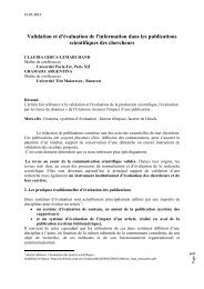
‣ s 0 S is a state called state of starting or an initial state;‣ F S is the set of final states, a (possibly empty) subset of S ( or state of acceptance).Definition 2.3.[4, 5] The modelling is a method used in science and technique, that involving the reproduction of anobject or system schematic form a system similar or analogous to studying the properties and transformations of theoriginal system. It can also be defined as a representation of a relationship by mathematical symbolism.Definition 2.4.[4, 5] The simulation is action to simulate a real system and results production its, the simulation hasthe purpose to find "something" about the mod of functioning of the system.Definition 2.5. [3] Is called Petri Nets a tuple S , T,Fin which :S T S T F (SxT) (TxS)so that : domF Im F S T.Elements of the set "S" are called places, elements of the set "T" are usually called transitions, and F iscalled flow relationship of the network . By here the name of the class of Petri Nets location-transition.Definition 2.6.[1, 2] Is called Coloured Petri Nets a tuple CPN = (P,T,A, ,V,C,G,E, I) where :1. S – represent a finite set, whose elements are called locations ( place ).2. T – represent a finite set, whose elements are called transition.The two sets must satisfy condition S T = .3. A S×T T ×S – represent the set of the arcs that connecting the locations at transitions and transitions atlocations.4. - represent a finite set of colors sets, different of set empty.5. V – represent a finite set of types of variables so that Type[v] for all variables vV.6. C : S→ - represent the function set of color, that assigns a set of color to each location.7. G : T →EXPRV – represent guard function that assign a guard to each transition t so that Type[G(t)] = Bool.8. E : A→EXPRV - represent function of the expression arc, that assign an expression of arc to every arc so thatType[E(a)] =C(s) MS , where s is location connected to the arc “a”.9. I : P→EXPR – represent initialization function that assign an initialization expression to each location s so thatType[I(s)] =C(s) MS .3 PRESENTATION OF THE MODEL.In the presentation the model we start from a deterministic finite state machine given, exemplified by asystem of activities which objects get the same type in two stages.We suppose there are two people A and B, the objects being processed of these persons. Person "A" toperform the first stage, and Person "B" executes the second stage. The objects obtained after the first stage are storedto be processed by the second person B.We suppose that the person "A" can take a break at any time, while Person B can take a break only if thereare not objects at process of work..A first modeling of this system can be seen in the table given :| t t1 21 2 t2t2_ ssss123s0f||||||_sssss1ffffThis modeling of the system can be interpreted more easily by viewing the DAF from Figure 1._sssssf22t 1 t 2ff_sssssff3ff_sssssfff2fs 1s { t 1 , t 1 2 2s 0 2 , t 2 } t 22

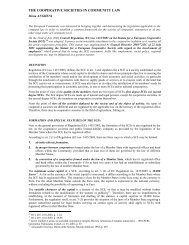
{ t 2 , t 2 1 , t 2 2 }{ t 1 , t 2 2 } t 22t 21s f s 3{t 1 , t 2 , t 2 1 , t 2 2 } {t 1 , t 2 }Fig 1.Finite state machine starts from state s 0 and by producing action t 1 this passes into state s 1 , otherwise said isconsidered that the objects were processed by actions t 1 objects that are stored in the state s 1 , i.e. the person "A"performing the first stage and the objects resulting are deposited in the state s 1 (DAF passes in state s 1 byproducing action t 1 ). Also, from state s 1 by producing one of the actions { t 1 , t 1 22 , t 2 } DAF can pass in the finalstate.By producing action t 2 the objects passing in state s 2 , the objects at this state include two posibilities:1) Person B can process objects – action t 2 enter loop. At this stage of work if it are produces one of theactions { t 1 , t 2 2 } DAF passes in the final state.2) Person B can take a break – which means that DAF passing in the state s 3 . At state s 3 either person Bresume work, by producing action t 2 2 , either DAF passes in the final state by producing one of the actions {t 1 , t 2 }.We note that DAF can reach the final state when are processed the sequences of instructions {t 1 , t 2 , t 1 2 , t 2 2 },but can't exactly surprise when the person can work and when the person can take a break.To highlight this situation we perform a new modeling of the system.This modeling of the system can be achieved by Petri network from Figure 2, where transitions and locationshave specifications given below.t22s 0 t 1 s 1 t 2s 2 s 3n• •In the location s 0 there are a number n of tokens. Conducting transition t 1 leads to processing of the objectsand their storage in the location s 1 . By producing transition t 2 , the second stage of work, objects are processed andstored in the location s 2 .Existence of a point in the location s 2 says that person B can do processing the objects, or to take a break.If occurs the transition t 1 2= persoa B enters the break.Existence of a point in the location s 3 says that person B enters the break (in this time person "A" canprocess objects). If the transition occurs t 2 2= person B return to work.Under the assumption that the person B may enter the break only if no objects to be processed, it followsthat the transition t 1 2must be permitted only at markings for which (s 1) =0. But, this can be achievedusing the classical rules of transition, because s 1 isn’t entry of the transition t 1 2 .Following this modeling we see the same situation encountered at modeling with the DAF. To avoid thissituation we make a new modeling, modeling made by Petri Nets with inhibitors.To achieve this new modelling is necessary to define these networks and their rules of operation.Definition 3.1[3] We call Petri Nets with inhibitors, abbreviated iPTN, the pair =( Σ,I) in which we have thesystem Σ’ =(S,T,F, ) that represent a Petri Nets, PN, iar I ⊂ S x T so that F∩i= , that specific the locations areattached to each transition.By marking of the network means any marking of the structure Σ and the sets markings of the network denoted by N S .Definition 3.2[3] Let Net =(Σ,I ) be a Petri Nets with inhibitors, iPTN, a marking own and t∈T.Fig 21t23

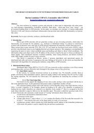
1) We say that transition t is enabled at the marking , we note [t> ia) [t > b) (s) = 0, ∀s∈S so that (s,t) ∈i.2) We say that marking ’ of the network is i- obtained by production trasition t at the marking , wea)[t inote [t> i ’ b)' (,t)We observe that at the classical rule by allow of the transition was attached a new rule of restriction and weobtained the rule de i-affordability, while the new rule of computing of the marking was not changed.When network is sub-understood we will use notations [t> i and [t> i ’ .Condition F∩i = from definition of Petri nets with inhibitors, iPN, is necessary because otherwise, if∃(s,t) ∈ F∩ i then t could not be i– possible at any marking of the network for that on of a side (s) =0and on of another side from [t> Σ ⇒ (s) ≥Pre (•,t)≥1, for that (s,t) ∈F what obviously is not possible.Let be Nets =(Σ,i), a Petri Nets with inhibitors, iPN, and ∈N S a marking own.Notions of :i sequence of transitions enabled at markingmarking i enabled from ⇔are defined as in the classicalcase. We obtained such the sets T( , ),TS( , ) and RM( , )which are equivalent to those of theclassic case.These networks are plotted as : , is represented as if classical,‣ Σ,0‣ M will be listed separately,‣ i is represented by draw to each (s,t) ∈i, an arc from s at t of form:| | ; s t.With those remarks the system of activities described above is shaped by miPN as in Figure 3.2t2s 0 t 1 s 1 t 2s 2 s 3n• •| |Fig. 3This network is equivalent with Petri Nets location / transition, which means that activities that occurringwithin its network are identical to those performed previously, but more than shows an inhibitory arc that allowsexecution of prioritized transitions and such the person "B" may stop the work or resume the work in a wellcontrolled manner..However, network evolution can not be seen in all her amplitude. Thus for a better view and observation of theevolution of the whole network we use a new class of Petri Nets, Colored Petri Net class, which shows multiplefacilities for modeling, validation and simulation of the systems.Using a tool provided by this class, CPN-Tools [8], whose license is provided by the CPN group at AarhusUniversity in Denmark, we construct a equivalent network to Petri Nets above.1t24

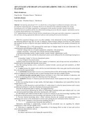
Fig. 4Network is composed of locations, transitions and arcs which have the following meanings:Locations :PROD – location of storage in which there are objects of the processed.A – location in which the person "A", puts the objects processed.BL – location in which the person B puts objects processed by it.BP – location in which the person B, if has not are objects of processed can take a break..Transitions :t 1 – action by which objects are processed by the person A and stored in location PROD.t 2 – action by which objects are processed by the person B and stored in location BL.t 3 – action by which person B can resume work.The arcs do connecting between transitions and locations or between locations and locations and can be printed withexpressions of arc.Evolution of the network can be interpreted thus:In the location PROD we have initial mark 20` 0e, otherwise said, here there are 20 objects ofprocessed. The first stage of processing is done by producing transition t 1 , objects processed are stored in thelocation A and at this moment is allowed and the transition t 2 , as can be seen in Figure 5.Fig. 5According with the hypothesis at this moment of the evolution of the network, the person "A" and the person "B"can handle objects. Stage two of processing of the objects is based on making transition t 2 that move objectsprocessed in the location BL. After making transition t 2 person B has two possibilities:a ) can enter the break, because in the location "A" there are not objects of processed.b) may resume work by producing transition t 3 , so how very easy can be seen from Fig. 6.5

Fig. 6At this stage modeling of the system is apparent that all requirements of the problem are easily observed.Presentation modeling the system by the four forms comes to show that using Colored Petri Nets in modeling,validation and simulation of the systems can be made quite easy, with low cost and remarkable results.CONCLUSIONS.This paper aims to highlight the dynamics development of the IT domain, as well as the latest news thatoccur every day in this area, which if known in time can facilitate substantially the activities in all fields.Besides multiple opportunities for modeling, simulation and validation provided by Coloured Petri Netsclass, this class generalized of the Petri Nets, provides a new software known as CPN-Tools, which by the useproper can provide vital informations about the system modeled, such as : references about the properties ofreachability, liveness, boundedness, fairness, deadlock, etc.REFERENCES[1].K. Jensen, “Coloured Petri Nets”, Vol 1,2,3 Spinger-Verlag Berlin Heidelberg, 1992.[2].K. Jensen, L. M. Kristensen,“ Coloured Petri Nets-Modelling and Validation of Concurrent Systems”,Spinger-Verlag Berlin Heidelberg, 2009.[3]. M. Popa, “Note de curs”, Bucuresti, 2008.[4].E. Gutuleac, “Modelarea si Evaluarea Performantelor Sistemelor de Calcul prin Retele Petri”, Dep. Ed.Poligrafic al UTM, Chisinau, 1997.[5]. Dictionar Encicopedic, Editura Enciclopedica Bucuresti, Bucuresti, 2007.[6]. C.Cassandras, S.Lafortune, "Introduction to Discrete Event Systems". Kluwer, 1999.[7]. T. Kam, “Synthesis of Finite State Machines: Functional Optimization.” Kluwer Academic Publishers,Boston 1997.[8]. http://www.cs.au.dk/CPnets/CPN-Tools, 2009.6