Chapter 3: Hydraulics DRAFT - NRCS Irrigation ToolBox Home Page

EFH Chapter 3 Hydraulics August 2009ENGINEERING FIELD HANDBOOKChapter 3 (650.03) - HydraulicsAcknowledgmentsThis major chapter revision was prepared under the general direction of Claudia Hoeft,national hydraulic engineer, Natural Resources Conservation Service (NRCS),Washington, DC, with assistance from National Design, Construction, and SoilMechanics Center staff, NRCS, Fort Worth, TX. Bill Irwin, national design engineer(retired), NRCS, Washington, DC, provided direction in the early stages of chapterrevision.Gilberto Urroz, Ph.D., P.E., associate professor and researcher at Utah State University,Logan, UT, is the principal author of this manuscript. Larry Goertz, hydraulic engineer,M&E Consultants, Heidenheimer, TX, provided extensive edits.Extensive comments were supplied by Mike DiLuzio, civil engineer (retired), NRCS,Grand Junction, CO; Ben Doerge, civil engineer, NRCS, Fort Worth, TX; Jon Fripp,stream mechnics engineer, NRCS, Fort Worth, TX; Tony Funderburk, agriculturalengineer, NRCS, Fort Worth, TX; Morris Lobrecht, civil engineer (retired), NRCS, FortWorth, TX; Clarence Prestwich, agricultural engineer, NRCS, Portland, OR; RickSchlegel, agricultural engineer, NRCS, Woodward, OK; Chuck Schmitt, civil engineer,NRCS, Casper, WY; Marty Soffran, agricultural engineer (retired), NRCS, Salina, KS;Karl Visser, hydraulic engineer, NRCS, Fort Worth, TX; and Jerry Walker, agriculturalengineer, NRCS, Fort Worth, TX.August 20092

EFH Chapter 3 Hydraulics August 2009Table of Contents0300 Introduction.............................................................................................................. 110301 Dimensions and Units.......................................................................................... 110302 Unit Conversions ................................................................................................. 140303 Dimensional Homogeneity in Equations ............................................................. 140304 Physical Properties of Water................................................................................ 150310 Hydrostatics ............................................................................................................. 200311 Hydrostatic Pressure Relationships...................................................................... 200311.1 Piezometers and Manometers ........................................................................... 240312 Forces on Submerged Plane Surfaces.................................................................. 310313 Buoyancy Forces.................................................................................................. 360313.1 Buoyancy Applications..................................................................................... 360315 Hydrokinetics........................................................................................................... 400316 Flow Continuity ................................................................................................... 400317 Conservation of Energy ....................................................................................... 450317.1 Potential Energy................................................................................................ 460317.2 Pressure Energy ................................................................................................ 460317.3 Kinetic Energy .................................................................................................. 460317.4 Equation of Energy and Bernoulli’s Principle.................................................. 510317.5 Hydraulic and Energy Gradients....................................................................... 540320 Open Channel Flow ................................................................................................. 570321 Uniform Open Channel Flow............................................................................... 570321.1 Geometric Characteristics of Prismatic Channels............................................. 590321.2 Manning’s Equation.......................................................................................... 650321.3 Manning’s Resistance Coefficient .................................................................... 660321.4 Calculations in Uniform Flow .......................................................................... 680322 Specific Energy in Open Channels ...................................................................... 700322.1 Critical Flow ..................................................................................................... 730322.1.1 Flow Types…………………………………………………………………..750322.1.2 Critical Flow in a Rectangular Channel……………………………………..760322.2 Obstacles in Open Channels ............................................................................. 780323 Momentum Analysis in Open Channels .............................................................. 810323.1 Hydraulic Jumps ............................................................................................... 850324 Varying Open Channel Flow ............................................................................... 900324.1 Gradually-varied Flow………………………………...………………………910324.2 Classification of Gradually-varied Flow........................................................... 920324.3 Standard step method........................................................................................ 940325 Sediment Transport.............................................................................................. 960325.1 Sediment Properties .......................................................................................... 960325.2 Threshold of Sediment Motion ....................................................................... 1010325.3 Suspended Sediment Load.............................................................................. 1040325.4 Bed Sediment Load......................................................................................... 1070325.5 Scour and Deposition in Channels.................................................................. 1090330 Pipe Flow ............................................................................................................... 1140331 Friction Loss Methods ....................................................................................... 1150331.1 Manning’s Equation for Pipelines .................................................................. 1153

EFH Chapter 3 Hydraulics August 20090331.2 Darcy-Weisbach Equation and Friction Factor……………………...……….1200331.3 Laminar and Turbulent Friction Factor Equations.......................................... 1220331.4 Pipe Flow Solutions Using the Darcy-Weisbach Equation ............................ 1230331.5 Pipe Flow Solutions Using the Hazen-Williams Formula……………...........1250331.6 Local Losses in Pipelines................................................................................ 1300331.7 Pumps in Pipelines.......................................................................................... 1370331.7.1 Pump Operational Characteristics………………………………………….1380331.7.2 Pump Power and Efficiency………………..……….…..……….…………1390332 Pipelines and Networks...................................................................................... 1410332.1 Pipelines in Series........................................................................................... 1420332.2 Pipelines in Parallel......................................................................................... 1450332.3 Pipelines Converging at a Single Point………………………………………1470332.4 Pipeline Networks .......................................................................................... 1500333 Appurtenances in Pipelines and Networks ........................................................ 1500333.1 Air Vacuum and Release Valves .................................................................... 1500333.2 Air Vents…………………………….…………………………..…………...1540333.3 Pressure Control Valves.................................................................................. 1550333.4 Surge/Air Chambers........................................................................................ 1570333.5 Check Valves .................................................................................................. 1590334 Hydraulic Transients (Water Hammer) ............................................................. 1590335 Cavitation…………………………………………………..…………………..1610336 Culverts ............................................................................................................. 1640336.1 Culvert Flow with Inlet Control...................................................................... 1650336.2 Culvert Flow with Outlet Control................................................................... 1670337 Sprinkler Irrigation............................................................................................. 1700338 Microirrigation................................................................................................... 1720340 Water Flow Measurements .................................................................................... 1730341 Measurements in Pipelines……………………………………………..…….. 1730341.1 Orifice Meters………………………………………………………………..1730341.2 Venturi Meters ................................................................................................ 1760341.3 Nozzle Meters ................................................................................................. 1780341.4 Elbow Meters.................................................................................................. 1790341.5 Magnetic and Ultrasonic Meters..................................................................... 1810342 Measurements in Open Channels....................................................................... 1810342.1 Depth Measurements ...................................................................................... 1830342.2 Velocity Measurements .................................................................................. 1830342.2.1 Propeller/ Paddle Wheel Meters………………………………………..….1830342.2.2 Vortex Meter……………………………………………………………….1830342.2.3 Doppler (Acoustic) Meters………………………………..……………….1840342.2.4 Velocity Measurements with Floaters……………………………………..1840342.2.5 Laser Doppler and Particle-Velocity Measurements………………………1840342.3 Sharp-crested Weirs........................................................................................ 1840342.4 Broad-crested Weirs........................................................................................ 1900342.5 Submerged Weir Flow .................................................................................... 1920342.6 Flumes............................................................................................................. 1940342.6.1 Long-throated Flumes...……………………………………………………1944

EFH Chapter 3 Hydraulics August 20090342.6.2 Parshall Flumes..…………………………………………………………...1940370 Hydraulic Modeling............................................................................................... 1950371 Similarity Between Models and Prototypes....................................................... 1950372 Hydraulic Modeling in Enclosed Flows (Pipelines) .......................................... 1970373 Hydraulic Modeling in Open-Channel Flow ..................................................... 1980374 Limitations of Models………………………………………………………….199REFERENCES ............................................................................................................... 200List of ExhibitsExhibit 1 – Dimensions and units of measurement ........................................................ 202Exhibit 2 – Selected conversion factors for units of measurement................................. 203Exhibit 3 – The Greek alphabet ...................................................................................... 206Exhibit 4 – Physical properties of water......................................................................... 207Exhibit 5 – Variation of atmospheric pressure with elevation........................................ 209Exhibit 6 – Pipe-system analysis for pump selection....………………………………..210Exhibit 7 – Culvert flow solutions using nomograms………………………………….212List of TablesTable 1. Basic units of measurement in the S.I. and E.S. systems ................................... 12Table 2. Manning’s resistance coefficients for open channel flow .................................. 68Table 3. Types of uniform flow in open channels. ........................................................... 75Table 4. Shape factors for sediment settling velocity..................................................... 101Table 5. Values of Manning’s resistance coefficient for pipe ........................................ 119Table 6. Absolute roughness values for pipe materials .................................................. 121Table 7. Values of the Hazen-Williams coefficient........................................................ 127Table 8. Pipe entrance loss coefficients ......................................................................... 132Table 9. Local loss coefficients for selected pipe fittings............................................... 133Table 10. Local head loss coefficients for a sudden pipe contraction. ........................... 143Table 11. Effect of neglecting local losses on an example pipeline system................... 145List of FiguresFigure 1. Schematic of Newton’s viscosity experiment .................................................. 16Figure 2. Cavitation damage on the propeller of a Francis turbine. ................................ 19Figure 3. Schematic of pressure measurement in a liquid. .............................................. 20Figure 4. Pressures within a liquid at rest........................................................................ 22Figure 5. Calculation of pressures at different depths. .................................................... 23Figure 6. Simple manometer (piezometer) ...................................................................... 24Figure 7. Piezometers on a horizontal pipe flow. ............................................................ 25Figure 8. Piezometers near an orifice meter in a pipeline................................................ 26Figure 9. U-tube manometer............................................................................................ 26Figure 10. U-tube manometer for flow measurement in a pipeline................................. 28Figure 11. Schematic of manometric measurements at an orifice plate in a pipe. .......... 29Figure 12. Deformation manometer (Bourdon manometer)............................................ 30Figure 13. Force on a submerged horizontal surface....................................................... 315

EFH Chapter 3 Hydraulics August 2009Figure 14. Point of application of a force on a submerged horizontal surface. ............... 31Figure 15. Pressure distribution, force, and center of pressure on an inclined surface. .. 33Figure 16. Pressure prism (a) and force location (b) for a vertical rectangular surface .. 35Figure 17. Buoyancy and weight forces acting on a submerged body ............................ 37Figure 18. Flow continuity in a pipe expansion............................................................... 41Figure 19. Schematic of flow in branching pipelines. ..................................................... 42Figure 20. Non-symmetric trapezoidal cross-section in an open channel flow............... 43Figure 21. Contraction in a rectangular open channel. .................................................... 44Figure 22. Rectangular open channel diversion............................................................... 45Figure 23. Flow energies illustrated with a simple reservoir-sprinkler system ............... 46Figure 24. Energy heads in pipe flow. ............................................................................. 47Figure 25. Energy heads in open channel flow................................................................ 50Figure 26. Sluice gate flow. ............................................................................................. 52Figure 27. Schematic of uniform flow in open channels................................................. 57Figure 28. Non-symmetric trapezoidal channel............................................................... 60Figure 29. Channel cross-sections that can be derived from a non-symmetric trapezoidalcross-section...................................................................................................................... 61Figure 30. Circular cross-section in open channel flow. ................................................. 63Figure 31. Parabolic cross section………………………………...…………………….64Figure 32. Specific energy curve for a trapezoidal open channel.................................... 71Figure 33. Specific energy curve for a rectangular open channel.................................... 73Figure 34. Relationship of cross-sectional area dA, flow depth d(d), and top width T ... 74Figure 35. Types of uniform flow in open channels........................................................ 76Figure 36. Hump at the bottom of a horizontal rectangular channel. .............................. 78Figure 37. Forces and flow of momentum for sluice gate flow....................................... 81Figure 38. Conjugate depths in the unit momentum function diagram for a rectangularopen channel. .................................................................................................................... 84Figure 39. Hydraulic jump produced by a stilling basin at the base of a spillway. ......... 85Figure 40. Hydraulic jump observed at the foot of a model spillway (Courtesy of theUtah Water Research Laboratory). ................................................................................... 86Figure 41. Forces and flow of momentum for a hydraulic jump..................................... 86Figure 42. Hydraulic jump over a baffle block................................................................ 89Figure 43. Varying flow from a reservoir leading to uniform flow in an open channel..90Figure 44. Gradually-varied flow (GVF) near an overfall............................................... 92Figure 45. Gradually-varied flow (GVF) produced by a weir......................................... 92Figure 46. Classification of gradually-varied flow (GVF) .............................................. 93Figure 47. Gradually-varied flow (GVF) curves in a mild-slope open channel with asluice gate and overfall. .................................................................................................... 93Figure 48. Shield’s diagram for determining the threshold of sediment motion in openchannel flow.................................................................................................................... 102Figure 49. Channel bed degradation downstream of a dam due to reduction in sedimentsupply.............................................................................................................................. 109Figure 50. Pipe Flow calculations with the USDA-NRCS Hydraulics Formula. .......... 118Figure 51. Discharge from a pipe into a reservoir. ........................................................ 131Figure 52. Entrance loss coefficients for typical pipe entrance shapes ......................... 1326

EFH Chapter 3 Hydraulics August 2009Figure 53. Solution for pipe flow with entrance loss using USDA-NRCS HydraulicsFormula........................................................................................................................... 133Figure 54. Schematic of pipe flow between two reservoirs........................................... 134Figure 55. Solution to pipe flow including all local losses using USDA-NRCS HydraulicsFormula........................................................................................................................... 137Figure 56. Pump discharge-head graph. ........................................................................ 139Figure 57. System schematic showing motor M, electric supply E, and pump P.......... 140Figure 58. Three pipelines in series connecting two reservoirs..................................... 142Figure 59. Three pipelines in parallel connecting two reservoirs.................................. 146Figure 60. Three pipelines converging to a single delivery point.................................. 148Figure 61. Location and dimensions of air vent chamber near a water intake. ............. 154Figure 62. Schematic of pump-pipeline system protected with a surge chamber. ........ 158Figure 63. Siphon conduit connecting two reservoirs. .................................................. 161Figure 64. Flow regimes for submerged inlet flow in culverts...................................... 165Figure 65. Central pivot irrigation system near Grace, Idaho........................................ 171Figure 66. Schematic of a sprinkler system layout........................................................ 172Figure 67. Schematic of flow through an orifice plate in a pipe…………………….....173Figure 68. Contraction, velocity, and discharge coefficients for flow through orifices: (a)sharp thick wall, (b) rounded thick wall, (c) chiseled thin wall, (d) sharp thin wall. ..... 174Figure 69. Schematic of orifice plate............................................................................. 175Figure 70. Plexiglas pipe with an orifice meter and piezometric tubes, used in thelaboratory to demonstrate orifice flow............................................................................ 175Figure 71. Schematic of a Venturi meter....................................................................... 176Figure 72. Plexiglas Venturi meter with piezometric tubes to demonstrate flow throughthe meter.......................................................................................................................... 177Figure 73. Venturi meter installed in a 4-inch pipeline, with manometer lines attached atthe upstream end and at the throat of the meter.............................................................. 177Figure 74. Schematic of a nozzle meter......................................................................... 178Figure 75. Schematic of an elbow meter. ...................................................................... 180Figure 76. Values of the discharge can be interpolated graphically from the rating curveof a given device. ............................................................................................................ 181Figure 77. Depth gage showing water surface elevation. .............................................. 182Figure 78. Point gage in laboratory flume with Vernier scale reading of 23.7.............. 183Figure 79. Suppressed sharp-crested weir in a rectangular channel. ............................. 185Figure 80. Contracted sharp-crested weir in a rectangular channel............................... 185Figure 81. Sharp-crested weir in operation (USDA). .................................................... 186Figure 82. Contracted rectangular weir with n = 1 or n = 2 contractions. .................... 187Figure 83. Contracted weir in a laboratory flume.......................................................... 188Figure 84. Cipoletti weir schematic............................................................................... 188Figure 85. Schematic of a triangular or v-notch weir. ................................................... 189Figure 86. V-notch, or triangular, weir in a laboratory flume. ...................................... 189Figure 87. Schematic of flow over a broad-crested weir............................................... 190Figure 88. Submerged weir flow. .................................................................................. 192Figure 89. Coefficient of submergence for sharp-crested weirs.................................... 193Figure 90. Model and prototype quantities.................................................................... 1957

EFH Chapter 3 Hydraulics August 2009Figure 91. Prototype and model of an ogee spillway (courtesy of the Utah WaterResearch Laboratory, Utah State University). ................................................................ 196Figure 92. Riprap hydraulic model (source: USDA - ARS).......................................... 199List of ExamplesExample 1 – Pressure at depth in water............................................................................ 23Example 2 – Hydrostatic force on horizontal area............................................................ 32Example 3 – Hydrostatic force on inclined area .............................................................. 34Example 4 – Hydrostatic force on vertical gate................................................................ 36Example 5 – Buoyancy force calculation – depth of a loaded barge................................ 37Example 6 – Buoyancy force calculation – flotation safety of CMP inlet ....................... 38Example 7– Equation of continuity in a pipe - discharge and velocity calculation.......... 41Example 8 – Equation of continuity – velocity and discharge calculation in branchingpipeline.............................................................................................................................. 43Example 9 – Equation of continuity – velocity in a trapezoidal open-channel crosssection............................................................................................................................... 44Example 10 – Equation of continuity – channel width reduction..................................... 44Example 11 – Equation of continuity – rectangular open channel diversion ................... 45Example 12 – Calculation of pressure, velocity, piezometric and total head................... 48Example 13 – Calculation of total head............................................................................ 49Example 14 – Velocity head, specific energy, and total head in open-channel flow ....... 50Example 15 – Bernoulli’s principle applied to sluice gate flow....................................... 52Example 16 – Energy equation in pipelines ..................................................................... 53Example 17 – Energy equation in open channel flow ...................................................... 54Example 18 – Hydraulic and energy gradients in pipe flow............................................. 55Example 19 – Hydraulic and energy gradients in open channel flow .............................. 56Example 20 – Shear stress in uniform open-channel flow ............................................... 58Example 21 – Velocity calculation in open-channel flow using Chezy’s equation ......... 59Example 22 – Geometric characteristics of a non-symmetric trapezoidal cross-section .60Example 23 – Hydraulic radius for wide rectangular channel.......................................... 62Example 24 – Geometric characteristics of a symmetric trapezoidal cross-section in openchannels............................................................................................................................. 62Example 25 – Geometric characteristics of a circular cross-section in open channels .... 64Example 26 – Geometric characteristics of a parabolic cross-section.............................. 64Example 27 – Trapezoidal channel solution using USDA-NRCS Hydraulics Formulaprogram............................................................................................................................. 68Example 28 – Circular channel solution using USDA-NRCS Hydraulics Formulaprogram............................................................................................................................. 69Example 29 – Parabolic channel solution using USDA-NRCS Hydraulics Formulaprogram............................................................................................................................. 69Example 30 – Normal depth in a wide channel ................................................................ 70Example 31 – Specific energy diagram for a rectangular channel cross-section ............. 72Example 32 – Critical flow depth in a rectangular channel.............................................. 768

EFH Chapter 3 Hydraulics August 2009Example 33 – Critical slope in uniform open-channel flow with rectangular cross-section........................................................................................................................................... 77Example 34 – Change in channel bed elevation in a rectangular channel........................ 79Example 35 – Calculation of the Froude number in a rectangular channel...................... 80Example 36 – Rating curve for a broad crested-weir ....................................................... 81Example 37 – Momentum function diagram for a rectangular channel ........................... 83Example 38 – Calculation of force on sluice gate ............................................................ 84Example 39 – Discharge, head loss, and length of a hydraulic jump in a rectangularchannel .............................................................................................................................. 88Example 40 – Flow depth, head loss, and length of hydraulic jump in a rectangularchannel .............................................................................................................................. 88Example 41 – Calculation of force on an obstacle producing a hydraulic jump in arectangular channel ........................................................................................................... 89Example 42 – Gradually-varied flow calculation in a rectangular channel...................... 95Example 43 – Sediment size data analysis ....................................................................... 97Example 44 – Determining settling velocity of spherical sediments.............................. 100Example 45 – Determination of settling velocity for non-spherical sediments.............. 101Example 46 – Sediment motion threshold analysis using Shield’s diagram .................. 103Example 47 – Suspended sediment discharge calculation.............................................. 105Example 48 – Bed sediment load rate calculation.......................................................... 108Example 49 – Bed aggradation....................................................................................... 111Example 50 – Bed degradation downstream of dam ...................................................... 112Example 51 – Bed degradation with constant downstream elevation ............................ 113Example 52 – Pipeline discharge calculation using Manning’s equation....................... 117Example 53 – Pipeline discharge calculation using the USDA-NRCS Hydraulics Formulasoftware........................................................................................................................... 117Example 54 – Flow velocity in a helical corrugated metal pipe using Manning’s equation......................................................................................................................................... 119Example 55 – Head loss in a riveted and spiral steel pipe using Manning’s equation... 119Example 56 – Velocity in pipeline draining a reservoir – Manning’s equation ............. 120Example 57 – Reynolds number used to classify pipe flow ........................................... 122Example 58 – Pipe flow solutions with the Darcy-Weisbach equation.......................... 124Example 59 – Flow in pipeline draining a reservoir – Darcy-Weisbach equation ......... 125Example 60 – Pipe velocity calculation using the Hazen-Williams formula ................. 128Example 61 – Pipe discharge calculation using the Hazen-Williams formula............... 129Example 62 – Head loss calculation using the Hazen-Williams formula....................... 129Example 63 – Diameter calculation using the Hazen-Williams formula ....................... 129Example 64 – Flow in pipeline draining a reservoir – Hazen-Williams formula........... 129Example 65 – Pipe flow calculation including local losses using the USDA-NRCSHydraulics Formula software......................................................................................... 133Example 66 – Pipe flow between two reservoirs including local losses – Manning’sequation........................................................................................................................... 134Example 67 – Pipe flow calculation including local losses using USDA-NRCS HydraulicsFormula........................................................................................................................... 137Example 68 – Pump head and discharge analysis .......................................................... 138Example 69 – Pump power and efficiency calculation................................................... 1419

EFH Chapter 3 Hydraulics August 2009Example 70 – Pipes in series using the Darcy-Weisbach equation ................................ 144Example 71 – Pipes in series using the Manning’s equation.......................................... 145Example 72 – Pipes in series using the Hazen-Williams formula.................................. 145Example 73 – Pipes in parallel using the Manning’s equation....................................... 146Example 74 – Pipes in parallel using the Hazen-Williams formula ............................... 147Example 75 – Converging pipelines using Manning’s equation .................................... 148Example 76 – Converging pipelines using Hazen-Williams formula ............................ 149Example 77 – Air valve sizing........................................................................................ 151Example 78 – Air vent chamber sizing........................................................................... 155Example 79 – Pressure relief valve selection…………………………...……………...156Example 80 – Pressure reducing valve selection…...……...…………………………...157Example 81 – Surge chamber calculation....................................................................... 158Example 82 – Pressure increase with sudden closing of a valve.................................... 160Example 83 – Cavitation at high point of a siphon......................................................... 161Example 84 – Circular culvert calculation with design under inlet control ................... 166Example 85 – Circular culvert sizing.............................................................................. 168Example 86 – Culvert discharge calculation .................................................................. 169Example 87 – Flow discharge through an orifice meter................................................. 176Example 88 – Flow discharge through a Venturi meter ................................................. 177Example 89 – Flow discharge through a nozzle meter................................................... 179Example 90 – Flow discharge through an elbow meter.................................................. 180Example 91 – Flow velocity calculation using the float method.................................... 184Example 92 – Discharge over a suppressed rectangular weir......................................... 186Example 93 – Discharge over a suppressed rectangular weir......................................... 187Example 94 – Discharge over a contracted weir ............................................................ 187Example 95 – Discharge over a Cipoletti weir ............................................................... 189Example 96 – Discharge over a triangular weir.............................................................. 190Example 97 – Discharge over a broad-crested weir – critical depth measured.............. 191Example 98 – Discharge over a broad-crested weir – head measured ........................... 191Example 99 – Discharge over a submerged sharp-crested weir ..................................... 193Example 100 – Discharge through a Parshall flume....................................................... 195Example 101 – Geometric similarity calculations.......................................................... 196Example 102 – Control valve model calculation (pressurized flow).............................. 197Example 103 – Stilling basin model calculation (free-surface flow) ............................. 19810

EFH Chapter 3 Hydraulics August 20090300 IntroductionThis chapter presents the hydraulic principles that apply to the design and operation ofsoil and water conservation measures. The chapter contains sections on dimensions andunits, principles of water at rest (hydrostatics), and principles of water in motion(hydrokinetics). It also discusses the application of these principles to flow of water inpipes and open channels. The chapter also presents the more common methods ofmeasuring flow of water in open channels and pipes.0301 Dimensions and UnitsThe word “dimensions” refers to physical quantities involved in describing a physicalsystem. The basic dimensions of length (L), time (T), and mass (M) can be selected. Inthe analysis of hydraulic problems many derived quantities are used that combine thesebasic dimensions. Some of these derived quantities are listed next: Velocity: V = L/T (velocity = length/time) Acceleration: a = V/T = L/T 2 (acceleration = velocity/time) Force: F = Ma = ML/T 2 (force = mass acceleration) Momentum: I = MV = ML/T (momentum = mass velocity) Work or energy: E = FL = ML 2 /T 2 (work = force length) Power: P = W/T = ML 2 /T 3 (power = work/time)The definition of force given above, referred to as Newton’s second law of motion,indicates that the force F required to provide an acceleration to a body of mass m is givenby F = m a. In terms of the basic dimensions (L, T, M), a force has dimensions ofML/T 2 , as indicated above. Sometimes, force (F) is used as a basic dimension togetherwith L and T, and mass (M) is considered a derived quantity. In such case, the basicdimensions are (L, T, F) and mass has dimensions of M = FT 2 /L.Velocity and acceleration have the same dimensions when either mass or force isconsidered a basic dimendsion. Using (L, T, and F) as basic dimensions, the followingderived quantities are written: Momentum: I = MV = (FT 2 /L)(L/T) = FT Work or energy: E = FL Power: P = W/T = FL/TThe basic dimensions and the derived quantities referred to above are described in termsof units of measurement. There are two commonly used systems of units in modernengineering practice: the International System (referred to as S.I., or SystemeInternationale, in French) and the English System (referred to as E.S., and also known asthe Imperial System of units). The International System uses length, time, and mass(L,T,M) as the basic dimensions, while the English System uses length, time, and force(L,T.F) as the basic dimensions. The following table shows the basic units in bothsystems:11

EFH Chapter 3 Hydraulics August 2009Table 1. Basic units of measurement in the S.I. and E.S. systemsSystem of units Length Time Mass ForceInternational System (S.I.) meter (m) second (s) kilogram (kg) --English System (E.S.) foot (ft) second (s) -- pound (lb)Besides the foot, the inch (in), the yard (yd), and the mile (mi) are commonly-used unitsof length in the E.S. These units are defined as follows:1 in = 1/12 ft, or 1 ft = 12 in1 yd = 3 ft1 mi = 5280 ftTo define the unit of force in the S.I. or the unit of mass in the E.S. it is necessary to usethe acceleration of gravity (g), a quantity that is essentially constant on the surface of theEarth and has the valueg = 32.2 ft/s 2 =9.806 m/s 2With this acceleration we can define the weight of a given mass M as: Weight: W = Mg (weight = mass gravity)This relationship allows the definition of a unit of force in the S.I., the newton (N), defined as:1 N = (1 kg) (1 m/s 2 ) = 1 kgm/s 2Similarly, by using the expression for mass in terms of weight: Mass: M = W/gThe unit of mass in the E.S., the slug, can be defined as:1 slug = (1 lb)/ (1 ft/s 2 ) = 1 lbs 2 /ftIn the United States, the English System is the most commonly used system of units. Therefore,most of the problems presented in this chapter are worked using units of the English System. Thefollowing are basic units of the English System for the derived quantities presented earlier: Velocity: 1 ft/s = 1 fps Acceleration: 1 ft/s 2 Mass: 1 slug = 1 lbs 2 /ft. Momentum: 1 slugft/s = 1 slugfps = (1 lbs 2 /ft)(1 ft/s) = 1 lbs Work or energy: 1 lbft Power: 1 lbft/s12

EFH Chapter 3 Hydraulics August 2009where W represents weight (in the English system, the pound, lb, is commonly used tomeasure weight), and Vol represents volume. In dimensional terms, using (L, T, and F)as basic dimensions, one can write:W F 3[ ] [ Vol]L3 FLwhile [Q] = L 3 /T = L 3 T -1 , and [H] = L. Thus, from the equation defining power, one canwrite:[P] = [] [Q] [H] = (FL -3 ) ( L 3 T -1 ) (L) = FLT -1Exhibit 1 shows that the dimensions of [P] = FLT -1 ; thus, the equation P = QH is shownto be dimensionally homogeneous.Manning’s equation (see section 0321.2) illustrates an equation that is not dimensionallyhomogeneous. The equation is given by:VCu 2 / 3 1/ 2 R S0[Eq. 3]nwhere V is the velocity, C u is a constant, R is the hydraulic radius and has dimensions oflength, and S o is the channel bed longitudinal slope and is a dimensionless quantity, and nis the Manning’s resistance coefficient, another dimensionless quantity.From the equation, one may obtain the dimensions of V as:[V] = L 2/3However, from Exhibit 1, [V] = LT -1 . Thus, Manning’s equation is not dimensionallyhomogeneous. Although not dimensionally homogeneous, the empirical Manning’sequation has proven to be very successful in modeling flow in open channels andpipelines.0304 Physical Properties of WaterExhibit 4 presents tables with physical water properties (values may be interpolated fordifferent temperatures) defined as follows:Density is the mass per unit volume:MVol [Eq. 4]Units of density in the S.I. are kg/m 3 , while in the E.S., they are slug/ft 3 .15

EFH Chapter 3 Hydraulics August 2009Specific Weight is weight per unit volume (see equation 2): Units of specific weight in the S.I. are N/m 3 , while in the E.S., they are lb/ft 3 or pcf(pounds per cubic feet).Because weight is defined as W = Mg, where g is the acceleration of gravity, one can alsowrite = (W/Vol) = (Mg/Vol) = (M/Vol)g = g:WVol g[Eq. 5]Specific gravity is the ratio of the density of any fluid to that of water at 39.2 o F (4 o C).Water density tends to increase with decreasing temperature to a maximum value at39.2 o F (4 o C). As the temperature decreases further, the density of water decreases untilthe water turns into ice at 32 o F or 0 o C. Referring to the density of water at 39.2 o F or 4 o Cas w = 1000 kg/m 3 = 1.94 slug/ft 3 , or to its corresponding specific weight as w = 9806N/m 3 = 62.4 lb/ft 3 , the specific gravity of any fluid of density or specific weight , isdefined as:S [Eq. 6]wwFor example, mercury (chemical symbol = Hg), a liquid metal often used in pressuremeasurements in hydraulic laboratories, has a specific weight, = 846.14 lb/ft 3 .Therefore, the specific gravity of mercury isS 846.16lb/ ft 3 w62.4 lb / ft3 13.6Viscosity is a property that measures the ability of water to resist shear deformation. Thedefinition of viscosity can be understood by referring to an experiment that was firstconducted by Newton, in which a moving wall is driven at a constant velocity, V, througha quiescent water tank. A schematic top view is shown below:Figure 1. Schematic of Newton’s viscosity experimentMeasurements indicate that the local velocity varies linearly from zero at the fixed wall toV at the moving wall. Let F represent the force required to pull the moving wall, and A16

EFH Chapter 3 Hydraulics August 2009be the area of the wall in contact with the fluid. The shear stress on the moving wall isdefined as:F [Eq. 7]ANewton discovered that the shear stress is related to the velocity V and to the length H inthe tank through the following relationship:V [Eq. 8]HIn this equation, the quantity is referred to as the absolute or dynamic viscosity ofwater. The kinematic viscosity is defined by: [Eq. 9]The units of absolute or dynamic viscosity are Ns/m 2 = kg/(ms) in the S.I., and lbs/ft 2 inthe E.S. And, kinematic viscosity units are m 2 /s in the S.I. and ft 2 /s in the E.S. Noticethat the units of kinematic viscosity are those of area per unit time. The dimensions ofkinematic viscosity are [] = L 2 T -1 , i.e., they involve only kinematic quantities (area,which is length squared, and time), hence the name kinematic viscosity.For example, at a temperature of 70 o F, the kinematic viscosity of water is = 1.059x10 -5ft 2 /s, and its specific weight is = 62.3 lb/ft 3 . To determine the absolute or dynamicviscosity of water at that temperature, we use the formulas /g, and /g)= /g, where g = 32.2 ft/s 2 : g62.3lb 1.059103ft ft 32.22 s 5fts2 2.05 1052lb ft s4ft s2 2.05 105lb s2ftIn the technical literature there are references to two old units of viscosity, the poise ( P),a unit of dynamic viscosity, and the stokes ( St), a unit of kinematic viscosity. Theconversion factors for these units into units of the E.S. are:1 P = 2.088510 -3 lbs/ft 21 St = 1.07610 -3 ft 2 /sIn pipe flow, viscosity is used to define a quantity known as the Reynolds number:17

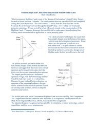
EFH Chapter 3 Hydraulics August 2009Figure 2. Cavitation damage on the propeller of a Francis turbine.Modulus of elasticity and water hammer. Bulk modulus of elasticity is a measure ofresistance of water to volume change under effect of pressure. Water and liquids, ingeneral, are referred to as incompressible fluids because they experience very smallvolume changes when subject to very large pressure changes. Gases, on the other hand,have large volume changes when pressure changes, and are, therefore, referred to ascompressible fluids. For any material, the bulk modulus of elasticity is defined as:pE [Eq. 11]V/ Vwhere p is the change in pressure applied to the material with initial volume V, and Vis the resulting change in volume. The negative sign in the equation signifies that anincrease in pressure (positive p) will produce a decrease in volume (negative V).Thus, the bulk modulus of elasticity can be defined as the change in pressure per unitchange in volume of a fluid.For example, at a temperature of 60 o F, the modulus of elasticity of water is E = 311000psi = 44784000 psf. If we wanted to reduce the volume of a water mass by V = - 0.1ft 3 , and given that the original volume is V = 1 ft 3 , the equation above indicates that therequired pressure increase is extremely large, namely:3V( 0.1ft ) p E 311000 311003V(1 ft ) psi psi19

EFH Chapter 3 Hydraulics August 2009This calculation illustrates that water (and liquids, in general) are, for most practicalpurposes, incompressible. The incompressibility of water is a factor in producing aphenomenon known as water hammer (see section 0334).0310 HydrostaticsHydrostatics refers to the study of water (and other liquids) at rest. Such is the case, forexample, of water contained in a storage tank with no flow in or out. Subjects of interestin hydrostatics include determination of pressures in a fluid, instruments for measuringpressure, calculation of forces on submerged surfaces (e.g., on gates or tank walls), andstudy of buoyancy.0311 Hydrostatic Pressure RelationshipsPressure is defined as the force per unit area that a fluid (liquid or gas) exerts on a surfacesubmerged in the fluid. The pressures discussed here are those within a body of water atrest. Consider, for example, a water tank as shown in the figure below.Figure 3. Schematic of pressure measurement in a liquid.A small probe of area A is introduced at a point in the tank as shown. If the force that thewater exerts on the probe tip is F, then the pressure at that point isFp [Eq. 12]AChanging the orientation of the probe’s tip at the same point, does not change the forceexerted by the water on the tip. Thus, the pressure at any given point does not changewith the orientation of the surface acted upon. Pressure is said to be isotropic, i.e., it isindependent of the orientation in which it is measured.The following table lists some of the most commonly used units of pressure in theEnglish System (E.S.) and International System (S.I.). Notice that pressure can also be20

EFH Chapter 3 Hydraulics August 2009expressed in terms of the height of a liquid column as shown below. In this table, H 2 0and Hg are the chemical symbols of water and mercury, respectively.Unit of PressureDefinition or Equivalent__________Basic Unitspsf 1 lb/ft 2 = 0.006944 psi = 47.88 Papsi1 lb/in 2 = 144 psf = 6894.76 PaPa (Pascal)1 N/m 2 = 0.02088 psf = 0.000145 psiOther UnitskPa (kilo Pascal)MPa (mega Pascal)barmb (millibar)atm (atmosphere)1,000 Pa1,000 kPa = 1,000,000 Pa14.50 psi = 100,000 Pa0.001 bar = 0.014504 psi = 100 Pa14.7 psi = 101,325 PaHeight of Liquid Column1 m H 2 0 1.4209 psi = 9796.85 Pa1 ft H 2 0 0.4331 psi = 2986.08 Pa1 in H 2 0 0.03609 psi = 248.84 Pa1 mm Hg 0.01934 psi = 133.32 Pa1 in Hg 0.4912 psi = 3,386.39 Pa_______________________________________________________Pressure, within a liquid at rest, increases linearly with depth. Referring to Figure 4, ifthe pressure at elevation z 0 is known to be p 0 , then the pressure p at elevation z, is givenby the hydrostatic law:p = p 0 + zwhere is the specific weight of the liquid, and z = z-z 0 is the difference in elevation ofthe two points of interest. The elevations z and z 0 are measured from any commonhorizontal level or datum.21

EFH Chapter 3 Hydraulics August 2009h 3 = 20 ft – z 3 = 20 ft – 5 ft = 15 ftThen, using = 62.4 lb/ft 3 for the specific weight of water, the corresponding (gage)pressures are:lblb 312 lbp1 h1 62.4 5 ft 312 2. 2 psi322ftft 144 inlblb 624 lbp2 h2 62.410f 624 4. 3 psi322ftft 144 inlblb 936 lbp3 h3 62.415f 936 6. 5 psi322ftft 144 in0311.1 Piezometers and ManometersManometers are instruments used in the measurement of pressure. The simplestmanometer consists of a u-tube with a leg attached to the point where the pressure will bemeasured, and the other leg open to the atmosphere. Such a manometer is illustrated inFigure 6.Figure 6. Simple manometer (piezometer)The circle centered at B may represent, for example, the cross-section of a flowing pipe.The elevation of point A (open to the atmosphere) with respect of the pipe centerline B isequal to h. Suppose that the liquid (e.g., water) in the pipe and manometer has aspecific weight , then, according to the hydrostatic law, the pressure at B is given by:24

EFH Chapter 3 Hydraulics August 2009p B = p A + hIf we use gage pressure to report our result, then we can take p A = 0, and the pressure atthe pipe centerline will be simply:p B = hIn pipeline flow we are often interested in determining the so-called piezometric head ofthe flow at a given location. The piezometric head, as illustrated in Figure 6, above, isthe sum of the pressure head (h = p B /) plus the elevation of the pipe centerline z B .Thus, a manometer, as the one illustrated above, is also known as a piezometer, for itshows the piezometric head in a pipe flow.In many cases, piezometers are simply vertical tubes attached to the top of the pipeline,as illustrated in the figure below.Figure 7. Piezometers on a horizontal pipe flow.The piezometers in Figure 7 above show the location of the hydraulic grade line (HGL),which, in a horizontal pipeline, illustrates the decrease in pressure along the pipeline inthe direction of the flow. The piezometers in the figure show that the piezometric headdecreases from A to B to C, thus, h A > h B > h C . The centerline elevation of points A, B,and C is the same, i.e., z A = z B = z C , therefore, the pressure heads (for point A, thepressure head is h A – z A ) will be such that h AP > h BP > h CP .25

EFH Chapter 3 Hydraulics August 2009The photograph in Figure 8, below, shows piezometers located before and after an orificemeter in a transparent pipeline, typically used in a laboratory setting. An orifice meter isused to measure flow discharge in a pipe. The piezometers are used to measure thepressure variation about the orifice meter.Figure 8. Piezometers near an orifice meter in a pipelineThe figure below shows a u-tube manometer being used to determine the pressure at thecenterline of a flowing pipe (point C). The flowing fluid has a specific weight 1 , whilethe manometric fluid has a specific weight 2 .Figure 9. U-tube manometerFor the case shown in Figure 9, above, point A is open to the atmosphere, thus, usinggage pressures, we can write p A = 0. The interface between the two liquids, point B, is26

EFH Chapter 3 Hydraulics August 2009called a meniscus. Point B is located at a depth h 2 with respect to the free surfacemeniscus A. Thus, the gage pressure at point B can be calculated as:p B = p A + 2 h 2 = 0 + 2 h 2 = 2 h 2On the other hand, within the flowing fluid, the pressure at point B can be written as(hydrostatic law):p B = p C + 1 h 1Equating the two expressions found above for p B one can write:p C + 1 h 1 = 2 h 2from which it follows that:p C = 2 h 2 - 1 h 1If the flowing fluid is water, 1 = w (the specific weight of water), and 2 = S m w ,where S m is the specific gravity of the manometric fluid (e.g., for mercury, S m = 13.56).Thus, one can write:p C = S m w h 2 - w h 1 = w (S m h 2 - h 1 )For example, to determine the pressure at point C in the figure above, given that themanometric fluid is mercury (S m = 13.56), and that h 2 = 6 in = 6/12 ft = 0.5 ft, h 1 = 2in = 2/12 ft = 0.167 ft, and w = 62.4 lb/ft 3 , using the equation above:p C = w (S m h 2 - h 1 ) = (62.4 lb/ft 3 )(13.560.5 ft – 0.167 ft) = 412.7 lb/ft 2 , or412.7 lbp C 2.87 psi 3psi2144 inThe photograph in Figure 10 shows a u-tube manometer used to measure flow dischargein the pipe located behind the manometer. The manometer legs in the photograph areattached to tubes connected to a Venturi meter (not shown). The manometric fluidshown is a red manometric fluid with a specific gravity S m = 0.75.27

EFH Chapter 3 Hydraulics August 2009Figure 10. U-tube manometer for flow measurement in a pipeline.Rules for manometer calculations. The following rules apply to the calculation ofpressures in tube manometers involving a number of fluids:Start at a point of known pressure or at a point where the pressure is required.Following the tube manometer to the next meniscus, add the product (specificweight depth) if the meniscus is located below the starting point, or subtract thesame product if the meniscus is located above the starting point.Continuing the path to the next meniscus, add the product (specific weight depth) if the meniscus is located below the previous meniscus, or subtract thesame product if the meniscus is located above the previous meniscus.When reaching the ending point in the manometer path, make the resulting sumequal to the pressure at the ending point.For example, for the piezometer in Figure 6, one can write:p A + h= p BFor the manometer of Figure 9, one can write:p A + 2 h 2 - 1 h 1 = p C28

EFH Chapter 3 Hydraulics August 2009As an additional example, consider the case in which a manometer at an orifice plate,illustrated in Figure 11, below.Figure 11. Schematic of manometric measurements at an orifice plate in a pipe.To determine the difference in pressures between points 1 and 2, use the rules formanometer calculations presented above; start at point 1 and first write:p 1 + w (d+h)The above expression reachs from point 1 to meniscus A using water for the specificweight. From point A to point B, use the specific weight of the manometric fluid, andsubtract the amount m h from the expression above, thus, producing:p 1 + w (d+h) - m hFrom point B to point 2, subtract the amount w d from the expression above, and makethe result equal to the pressure at point 2:Expanding the expression above:p 1 + w (d+h) - m h - w d = p 2p 1 + w d + w h - m h - w d = p 2Eliminating the terms + w d and - w d, one gets:p 1 + w h - m h = p 2Algebraic manipulation of this equation allows writing:p = p 1 – p 2 = ( m - w ) h29

EFH Chapter 3 Hydraulics August 2009The resulting equation can be simplified by introducing the specific gravity of themanometric fluid, i.e., m = S m w , thus:p = w h (S m -1)If w = 62.4 lb/ft 3 , h = 8 in = 8/12 ft = 0.666 ft, and S m = 13.56 (for mercury), thedifference in pressure, p is:p = w h (S m -1) = (62.4 lb/ft 3 )(0.666 ft)(13.56 - 1) = 521.97 lb/ft 2or lbp 521.973. 62 psi2144 inOrifice plates may be used to measure flow in pipelines. The pressure difference, p, canbe related to the pipeline discharge by calibration or by theoretical analysis. Examples ofsuch analyses are presented in the next section.Deformation Manometers. Deformation manometers, such as the Bourdon manometershown in the following figure, utilize the deformation of spiral tubes or of diaphragmsto measure pressure. These manometers are calibrated by manufacturers or in thelaboratory and provide a direct reading of the pressure at the manometric tap.Modern deformation manometers have digital readouts, making the reading of thepressure straightforward. The Bourdon manometer shown in Figure 12 has an analogscale, with the pressure marked by the pointer attached to the spiral tube located insidethe manometer.Figure 12. Deformation manometer (Bourdon manometer)30

EFH Chapter 3 Hydraulics August 20090312 Forces on Submerged Plane SurfacesThe calculation of the size, direction, and location of the forces on submerged surfaces isessential in the design of dams, bulkheads, water control gates, and other relatedappurtenances.Horizontal surface. The hydrostatic law indicates that pressure varies with depth. Thus,a horizontal surface within a liquid at rest is subject to the same pressure p over the entiresurface, and the resultant force F on the surface is given by:where, A is the area of the surface.F = pA = hA [Eq. 15]Figure 13. Force on a submerged horizontal surfaceFigure 13 shows that the pressure on top of the horizontal surface is represented byvertical arrows of the same height pointing towards the surface. The pressure arrows andthe horizontal surface form a three-dimensional figure known as the pressure prism. Theresultant force vector on any surface coincides with the centroid (also referred to as thecenter of mass or center of gravity) of the pressure prism. The force on a horizontalsurface will be vertical and applied to the centroid C of the surface as illustrated in Figure14, below. The point of application of the force is referred to as the center of pressure P.Figure 14. Point of application of a force on a submerged horizontal surface31

EFH Chapter 3 Hydraulics August 2009Example 2 – Hydrostatic force on horizontal areaA circular tank 15 ft in diameter is filled with water to a depth of 2 ft. Determine themagnitude and location of the vertical force that the water applies on the tank bottom.The tank has a diameter D = 15 ft, therefore, the area of the tank bottom is that of a circle: DA 423.1416(15 ft)42 176.71 ft2The magnitude of the pressure applied to the bottom of the tank can be calculated byusing the specific weight of water, = 62.4 lb/ft 3 and depth of the water in the tank, h =2 ft:p = h = (62.4 lb/ft 3 )(2 ft) = 124.8 lb/ft 2The magnitude of the force applied on the tank bottom is:F = pA = (124.8 lb/ft 2 )(176.71 ft 2 ) = 22053.41 lbThe force is applied at the center of the circular bottom and is equivalent to the weight ofthe water.Inclined surface. For a surface located on an inclined plane, the pressure increaseslinearly from the top of the surface to the bottom of the surface. The magnitude of theforce on the surface is calculated as:F = p c A = h c A [Eq. 16]Where p c = h c is the pressure at the centroid of the figure. The force, F, is representedby the volume of the pressure prism.Figure 15, below, shows the pressure distribution along an inclined surface and theresulting force on a rectangular region laid on the inclined surface. The rectangularregion could represent a gate on the slope of a dam or dike. The inclined surface islocated at an angle with respect to the horizontal. Alternatively, the slope can beindicated by the proportion zH(horizontal):1V(vertical) as shown in the figure. For thecase illustrated in Figure 15, the angle is related to the slope by:tan( ) b 1[Eq. 17]a zFigure 15 shows a system of coordinate axes, x and y, located on the inclined surface.The system is selected so that the x-axis is located along the free surface. Points on theinclined surface can be located by either their depth h or their y coordinate along thesurface. These two distances are related by:h y sin( )[Eq. 18]32

EFH Chapter 3 Hydraulics August 2009Point 1 is located at the top of the gate while point 2 is located at the bottom of the gate.The gate dimensions are B (width) and H (height). Point C represents the centroid of thegate, while point P represents the point of application of the hydrostatic force F on thegate, the center of pressure.Figure 15. Pressure distribution, force, and center of pressure on an inclined surface.Unlike the case of a horizontal surface, the center of pressure on an inclined surface islocated below the centroid of the surface along the plane of the surface, by a distancegiven by:Ic y [Eq. 19]A yIn this formula, y c is the location of the centroid of the surface measured from the freesurface along the plane of the surface, and I c is the moment of inertia of the surface withrespect to a centroidal axis parallel to the x axis (i.e., an axis through point C). Thus, thecenter of pressure will be located at a distancecy p = y c + y =ycIc [Eq. 20]A ycFor the rectangular and circular figures of Figure 14, with the x axis representing thecentroidal axis x c , the centroidal moments of inertia are the following:Rectangular area:1 BH12I3c [Eq. 21]33

EFH Chapter 3 Hydraulics August 2009Circular area:I c64 D4 [Eq. 22]Since most gates are either rectangular or circular, equations 21 and 22 will be useful forcalculating the center of pressure of those types of gates by using equations 19 and 20.________________________________________________________________________Example 3 – Hydrostatic force on inclined areaFor the rectangular gate illustrated in Figure 15, B = 3 ft, H = 4.5 ft, a = 2, b = 1, y 1 = 5ft, determine the force on the gate and the location of the center of pressure.The slope is specified by the numbers a = 2 and b = 1, i.e., 2H:1V. The correspondingangle is calculated as: tan1 b tan a 1 1 2 26.57While the top of the gate is located at a distance y 1 = 5 ft measured along the slope, thebottom of the gate will be located at:y 2 = y 1 + H = 5 ft + 4.5 ft = 9.5 ftThe centroid is located midway between y 1 and y 2 :The depth of the centroid is:y1 y25 ft 9.5 fty c 7. 25 ft2 2h c = y c sin( ) = 7.25 ft sin(26.57 o ) = 3.24 ftThus, the pressure at the centroid is (equation 18):p c = h c = 62.4 lb/ft 3 3.24 ft = 202.18 lb/ft 2The area of the gate is:A = BH = 3 ft 4.5 ft = 13.5 ft 2 .The force on the gate (equation 16):F = p c A = 202.18 lb/ft 2 13.5 ft 2 = 2729.43 lbTo calculate the location of the center of pressure, start by calculating the centroidalmoment of inertia using equation 21:34

EFH Chapter 3 Hydraulics August 2009I c112BH31123ft (4.5 ft)3 22.78 ft4The distance between the centroid C and the center of pressure is calculated withequation 19:4Ic22.78 ft y 0. 23 ft .2Ay 13.5 ft 7.25 ftThe center of pressure is located at the distance (equation 20):cy p = y c + y = 7.25 ft + 0.23 ft = 7.48 ft.And the depth of the center of pressure is (equation 18):h p = y p sin() = 7.48 ft sin(26.56 o ) = 3.35 ft.________________________________________________________________________Vertical surface. In Figure 16, a rectangular surface of width B is located on a verticalplane and the free surface of the water reaches to a depth H.Figure 16. Pressure prism (a) and force location (b) for a vertical rectangular surfaceThe triangular distribution in Figure 16(b) represents the pressure distribution on thevertical surface. The pressure at the bottom is given by p B = H. The force F on thesurface is equal to the volume of the pressure prism: 1 1F pB H B BH 2 22 [Eq. 23]Using equations 20 and 21 and the area of this rectangular surface, A = BH, one canprove that the location of the center of pressure (point of application of the force) is givenby:35

EFH Chapter 3 Hydraulics August 2009yp2 hp H[Eq. 24]3Thus, the force is applied at 2/3 of the depth measured from the surface, or 1/3 of thedepth measured from the bottom as indicated in Figure 16 (b). Examples of this typesurface include vertical gates and flashboards.________________________________________________________________________Example 4 – Hydrostatic force on vertical gateA wooden vertical gate with a width of 10 ft is used to close a canal. If the water depthon the gate is 2.5 ft, determine the hydrostatic force on the gate and its location.For this case B = 10 ft, H = 2.5 ft, and = 62.4 lb/ft 3 , thus, the force is (equation 23):1 2 1 lb2F BH 62.4 10ft (2.5 ft) 1950lb32 2 ftThe force is located at a distance from the surface (equation 24):2 2yp hp H 2.5 ft 1. 67 ft3 3________________________________________________________________________The use of a spreadsheet application greatly facilitates calculation of forces on submergedplane surfaces.0313 Buoyancy ForcesBuoyancy is the upwards force experienced by solid bodies submerged in liquids orgases. Archimedes’ principle states that a solid body submerged in a fluid (i.e., liquid orgas) experiences a vertical upward force (the buoyancy force) equal to the weight of thevolume of fluid it displaces. Thus, the buoyancy force, F B , experienced by a body ofvolume V submerged in a fluid of specific weight , is given by:F B = V [Eq. 25]0313.1 Buoyancy ApplicationsA solid body submerged is also acted upon by its own weight, which can be calculated asW = s V [Eq. 26]where s is the specific weight (weight per unit volume) of the solid material.A solid body fully submerged in water is subject to its own weight W (equation 26) andthe buoyancy force (equation 25) exerted by the water on the solid body. Figure 1636

EFH Chapter 3 Hydraulics August 2009illustrates several possibilities in terms of force equilibrium when a solid body, fullysubmerged in water, is released.Figure 16. Buoyancy and weight forces acting on a submerged bodyIf the net resulting force, F R , on the body, i.e., the difference between its weight W andthe buoyancy force F B , is zero, the body is said to be neutrally buoyant and it will remainin place within the water as illustrated in Figure 16(a).The net resulting force, F R , is a downward force if the weight is larger than the buoyancyforce (W>F B ), i.e., if the specific weight of the solid is larger than that of water s > ,e.g., metal). In this case the solid body will sink into the liquid until reaching the bottomof a container, as illustrated in Figure 16(b).On the other hand, if the weight is smaller than the buoyancy force (W

EFH Chapter 3 Hydraulics August 2009400lbh 0.53 ft 0.5312in = 6.36 in362.4lb / ft 4 ft 3 ft________________________________________________________________________Example 6 – Buoyancy force calculation – flotation safety of CMP inletThe figure below shows a cylindrical CMP (corrugated metal pipe) vertical inlet ofdiameter d = 36 in = 3 ft, supported on a square footing of side length L, and height h b =13.5 in = 1.125 ft The inlet footing is covered with saturated soil up to a depth h = 7 ftwhich corresponds to the level of the inlet crest. The CMP inlet weighs CMP = 38 lb/ft,the buoyant weight of saturated soil on the footing is SS = 60 lb/ft 3 , and the concrete inthe footing weighs C = 150 lb/ft 3 . Determine the size L of footing required to make theCMP inlet safe from flotation with a factor of safety F.S.= 1.5. Assume that there is nofrictional resistance between the inlet walls and the surrounding soil, and that no shearforces act on the outlet conduit. The minimum length L must be L = d + 1ft to allow forplacement of reinforcing steel bars outside of the inlet with 3 in concrete cover and 2 inclearance between bars and inlet.The factor of safety, F.S. for this case, is defined as the ratio of the net downward forces(F d ) to the net upward forces (F u ):FF.S.FduHere, , indicates summation of forces. By requiring that the factor of safety be F.S. =1.5, the downward forces are 50% larger than the upward forces ensuring that the inletwill be safe from flotation.38

EFH Chapter 3 Hydraulics August 2009Using the minimum length of footing:L = d + 1ft = 3 ft + 1 ft = 4 ftThe downward forces in this problem include the weight of the inlet, W CMP , the buoyantweight of saturated soil, W SS , and the weight of footing, W C . With the minimum length,these forces are calculated as follows:W CMP = CMP (h+h b ) = 38 lb/ft ×(7 ft + 1.125 ft) = 308.75 lbW SS = SS (L 2 h – d 2 /4 h) = 60 lb/ft 3 × ((4 ft) 2 -3.1416× (3ft) 2 /4) × (7 ft ) = 3,751.19 lbThus,W C = C L 2 h b = 150 lb/ft 3 ×(4 ft) 2 ×1.125 ft = 2,700 lbF d = W CMP + W SS + W C = 308.75 lb + 3,751.19 lb + 2,700 lb = 6,759.94 lbThe upward forces include the buoyancy forces on the riser, F BCMP , and on the footing,F BC , which are calculated as:F BCMP = w (d 2 /4) h = 62.4 lb/ft 3 × (3.1416×(3 ft) 2 /4) ×7 ft = 3,087.56 lbF BC = w L 2 h b = 62.4 lb/ft 3 × (4 ft) 2 ×1.125 ft = 1,123.2 lb39

EFH Chapter 3 Hydraulics August 2009Thus,F u = F BCMP +F BC =3,087.56 lb + 1,123.2 lb = 4,210.76 lbThe factor of safety for a side of footing L = 4 ft is:Fd6,759.94 lbF . S. 1.61 1.5F4,210.76 lbuSince the factor of safety calculated is larger than 1.5 the CMP inlet should be safe forbuoyancy. If F.S. < 1.5, try a larger footing side length or height, and recalculate the sumof forces and the factor of safety until it is larger than the required value of 1.5.________________________________________________________________________0315 HydrokineticsHydrokinetics is the study of fluids in motion. Motion in fluids is produced by the actionof forces. For example, in pressurized pipelines pressure forces act as the driving forcesin the flow, whereas, in open channel flow, it is the weight of water mass (gravity forces)that produces the motion. In both cases, friction between the water and the walls of thepipe or channel act as opposing forces. In steady flows, driving and opposing forces arein equilibrium.The analysis of fluids in motion typically requires the determination of flow quantitiessuch as discharge or velocity, or the determination of a linear quantity such as pipediameter or flow depth in open channel flow. The determination of energy or headlosses is also an important aspect of the analysis of fluids in motion. These analyses havepractical applications in the operation of devices or systems through which fluids (water)flow, for example, irrigation pipes, outlet works from dams, and irrigation canals.The principles of flow continuity and of conservation of energy are used to analyze fluidsin motion.0316 Flow ContinuityThe equation of continuity represents a statement of conservation of mass in fluid flow.Consider, for example, a steady flow in a closed conduit of varying cross-section asshown in Figure 18 below. Let Q be the discharge through the conduit. The equation ofcontinuity for steady flow (i.e., Q = constant) states that:Q = V 1 A 1 = V 2 A 2 = V 3 A 3 [Eq. 28]where V 1 , V 2 , and V 3 represent the flow velocities at sections 1, 2, and 3 respectively.The areas of the corresponding cross-sections are A 1 , A 2 , and A 3 .40

EFH Chapter 3 Hydraulics August 2009Figure 18. Flow continuity in a pipe expansion.The cross-sectional area of a circular pipe of diameter D is given by:2A D[Eq. 29]4And the discharge can be written as:2DQ VA V [Eq. 30]4Knowing the discharge Q, the velocity V in a circular conduit of diameter D can becalculated as:V4Q [Eq. 31]2DIn units of the English System, the velocity V is given in ft/s (or fps), while the dischargeQ is given in ft 3 /s or cfs. Using the International System, the velocity V is given in m/sand the discharge Q is given in m 3 /s. Other units of discharge in the English Systeminclude gal/min (or gpm) and gal/day (or gpd), which are commonly used in water supplyapplications. In the operation of large reservoirs, for example, the use of acre-foot/dayas a unit of discharge is not uncommon. In the International System one could also usem 3 /min or m 3 /day for large discharge operations, while the units of liters/s or liters/minare used for small discharges.________________________________________________________________________Example 7 – Equation of continuity in a pipe - discharge and velocity calculationSuppose that in the pipeline of Figure 18 the diameters are D 1 = 0.25 ft (3 in), D 2 = 0.50ft (6 in), and D 3 = 0.75 ft (9 in), and that the velocity at section 3 is measured to be V 3 =0.5 fps. Find the velocities in sections 1 and 2 and the discharge.The discharge is calculated as:41

EFH Chapter 3 Hydraulics August 200922D33.1416(0.75 ft)Q V3 0.5 ft / s 0. 22cfs44The velocities at sections 1 and 2 are, therefore, calculated as:and34Q40.22 ft / sV1 4. 48 fps22D 3.1416(0.25 ft)134Q4 0.22 ft / sV2 1. 12 fps22D 3.1416(0.5 ft)2________________________________________________________________________A branching pipeline in which a pipe of diameter D 1 splits into two pipelines withdiameters D 2 and D 3 is shown below. Continuity requires that the discharges throughsections 2 and 3 add to equal the discharge through section 1:Q 1 = Q 2 + Q 3 [Eq. 32]Figure 19. Schematic of flow in branching pipelines.In terms of areas and velocities, the continuity equation for the branching pipe case iswritten as:V 1 A 1 = V 2 A 2 + V 3 A 3 [Eq. 33]Replacing the areas in terms of the diameters:Simplifying:222D1D2D3V1 V2 V3[Eq. 34]4 4 442

EFH Chapter 3 Hydraulics August 2009V 1 D 1 2 = V 2 D 2 2 + V 3 D 32[Eq. 35]_______________________________________________________________________Example 8 – Equation of continuity – velocity and discharge calculation in branching pipelineA 12-in-diameter pipeline carrying water at a velocity of 3.5 fps branches into a 6-indiameterpipeline and a 9-in-diameter pipeline. If the velocity in the 6-in pipeline ismeasured to be 4.0 fps, what is the velocity in the 9-in pipeline, and what is the totaldischarge through the 12-in pipeline?Using D 1 = 12 in = 1 ft, V 1 = 3.5 fps, D 2 = 6 in = 0.5 ft, V 2 = 4.0 fps, and D 3 = 9 in =0.75 ft, find V 3 and Q 1 . From equation 35, i.e., V 1 D 1 2 = V 2 D 2 2 + V 3 D 3 2 , it follows that:2 222V1D1V2D23.5 fps (1 ft) 4.0 fps (0.5 ft)V3 4. 44 fps22D(0.75 ft)The discharge through section 1 is:322D13.1416(1 ft)Q1 V1 3.5 fps 2. 75cfs44________________________________________________________________________The equation of continuity can also be applied to flow in open channels. Consider theflow in an open channel with a non-symmetric trapezoidal cross-section as illustrated inthe figure below.Figure 20. Non-symmetric trapezoidal cross-section in an open channel flow.This cross-section is characterized by the bottom width b, the side slopes z 1 and z 2 , andthe flow depth d. The side slopes are interpreted as z 1 H:1V, i.e., z 1 units horizontal to 1unit vertical. The top width T is the length of the free surface at the cross-section. Forthe non-symmetric trapezoidal cross-section shown above, the top width is given byT = b + (z 1 +z 2 )d [Eq. 36]and the area is calculated as the average of trapezoid’s bases, b and T, multiplied by theheight of the trapezoid, d :T bA ( ) d2 bz1 z22d d[Eq. 37]43

EFH Chapter 3 Hydraulics August 2009________________________________________________________________________Example 9 – Equation of continuity – velocity in a trapezoidal open-channel cross-sectionSuppose that the non-symmetric trapezoidal cross-section of Figure 20 has b = 3 ft, d =1.3 ft, z 1 = 0.5, and z 2 = 1, and carries a discharge Q = 15.2 cfs. The area is calculatedas:A bz z2 0.5 1 2 1 2d d 3 ft 1.3 ft 1.3 ft 5. 17ft2And the flow velocity is: V = Q/A = 15.2 cfs/5.17 ft 2 = 2.94 fps________________________________________________________________________Example 10 – Equation of continuity – channel width reductionThe figure below shows a rectangular open channel that reduces in channel width from b 1to b 2 .Figure 21. Contraction in a rectangular open channel.In Figure 21 suppose that b 1 = 7.5 ft, and b 2 = 5.0 ft. The depth of flow and velocity insection (1) are d 1 = 2.5 ft and V 1 = 4.5 fps. What depth of flow is required in section (2)in order to maintain the same flow velocity (i.e., V 2 = V 1 = 4.5 fps)? What is the flowdischarge through the channel?With the cross-sectional shape being rectangular in both sections (1) and (2), the area ofthe cross-section is given by A = bd. Thus, the continuity equation (equation 28) can bewritten as:Q = V 1 b 1 d 1 = V 2 b 2 d 2The depth at section (2) is given by:d2V1b1d14.5 fps 7.5 ft 2.5 ft = 3.75 ftV b 4.5 fps 5.0 ft22The discharge is calculated as:Q = V 1 b 1 d 1 = 4.5 fps 7.5 ft 2.5 ft = 84.38 cfs44

EFH Chapter 3 Hydraulics August 2009________________________________________________________________________Example 11 – Equation of continuity – rectangular open channel diversionFigure 22 shows a rectangular channel of width b 1 from which water is diverted througha lateral rectangular channel of width b 3 . The section of the main channel downstreamfrom the diversion has a width b 2 = b 1 .Figure 22. Rectangular open channel diversion.Using b 1 = b 2 = 10 ft, d 1 = 4.0 ft, V 1 = 1.2 fps, d 2 = 3.5 ft, b 3 = 5.0 ft, d 3 = 2.5 ft, and V 3= 0.6 fps, determine the flow velocity at section 2, V 2 , as well as, the discharges throughsections 1, 2, and 3.For a branching channel as shown in Figure 22, continuity requires that Q 1 = Q 2 + Q 3 ,i.e., V 1 b 1 d 1 = V 2 b 2 d 2 + V 3 b 3 d 3 . Thus, the velocity at section 2 is:V 2 = (V 1 b 1 d 1 - V 3 b 3 d 3 )/(b 2 d 2 ) = (1.2 fps10 ft4 ft – 0.6 fps5 ft2.5 ft)/(10 ft3.5 ft) =V 2 = 1.157 fpsThe discharges through the three sections are calculated as follows:Q 1 = V 1 b 1 d 1 = 1.2 fps10 ft4 ft = 48 cfsQ 2 = V 2 b 2 d 2 = 1.157 fps10 ft3.5 ft = 40.5 cfsQ 3 = V 3 b 3 d 3 = 0.6 fps5 ft2.5 ft = 7.5 cfs________________________________________________________________________0317 Conservation of EnergyIn the analysis of fluid flow, three types of energy are typically considered: potential orelevation energy, pressure energy, and kinetic energy. Figure 23, below, illustrates theseconcepts using a simple reservoir-sprinkler system.45

EFH Chapter 3 Hydraulics August 2009Figure 23. Flow energies illustrated with a simple reservoir-sprinkler systemThe elevation of the water in the reservoir represents potential energy since it is thiselevation that provides the available energy for the system. As the water flows throughthe pipe and is discharged through the sprinkler, it acquires motion which converts someof the potential energy into kinetic energy (energy of motion). Also, at the sprinkler, ameasurable pressure exists that is related to pressure energy at that particular point.In a flowing fluid system as the one illustrated above, energy is conserved as it isconverted from one type of energy (potential) into another (pressure or kinetic). In fluidflow these energies are typically converted to energy heads that can be easily visualizedas in the potential energy head of Figure 23. The description of these energy headsfollows in the next sections.0317.1 Potential EnergyPotential energy is the ability of a water mass to perform work because of the elevation ofthat mass of water with respect to an arbitrary datum line or reference level. A mass ofweight W, at an elevation of z feet, has a potential energy equal to Wz (ft-lb) with respectto the datum. The elevation head, z, expresses not only a linear quantity (ft), but alsoenergy per unit weight, i.e., ft-lb/lb = ft.0317.2 Pressure EnergyPressure energy at a point of a fluid flow is produced by the local pressure at the point.This pressure could be the result of a pumping action in a pipeline or of the weight ofwater above a certain point in open channel flow. The pressure head (pressure energy perunit weight) in pipeline flow is calculated as p/, pressure divided by the specific weightof water. In open channel flow applications, the pressure head is equal to the flow depth,d, and the pressure distribution is assumed to be hydrostatic.0317.3 Kinetic EnergyThe kinetic energy (K) of a mass (M) of fluid moving at a velocity (V) is given by K =1/2MV 2 . Since its weight is W = Mg, the kinetic energy per unit weight is calculated as:46

EFH Chapter 3 Hydraulics August 20091 2MV 2h KV 2vW Mg 2[Eq. 38]gWhere g is the acceleration of gravity (g = 32.2 ft/s 2 ). The term h v in equation 38 isreferred to as the velocity head.The total energy head, H, is the sum of the potential energy head (z), the pressure head(p/ or d), and the velocity head (V 2 /2g). All three forms of energy head may beexpressed as a linear quantity (ft), or as energy per unit weight (ft-lb/lb).Energy heads in pipe flow. Figure 24 illustrates the three different energy heads appliedto pipe flow. Notice that, typically, the potential energy head (elevation) in a pipe flow isreferenced at the centerline of the pipe. The pressure head is measured from the pipecenterline, and the distance from the datum to the top of the pressure head represents thepiezometric head:ph z [Eq. 39]The difference between the total energy head and the piezometric represents the kineticenergy. The total energy in a pipe flow is given by:22V p VH h z [Eq. 40]2g 2gThe line representing the values of the total head, H, as function of position x along thepipeline is referred to as the Energy Line (E.L.), while that representing the values of thepiezometric head, h, is referred to as the Hydraulic Grade Line (H.G.L.). Energy losses,h f , are the losses due to friction between sections (1) and (2).Figure 24. Energy heads in pipe flow.47

EFH Chapter 3 Hydraulics August 2009________________________________________________________________________Example 12 – Calculation of pressure, velocity, piezometric and total headA manometer located at a point of a 6-in-diameter pipe shows a pressure reading of 6 psi.The point of pressure measurement is located at an elevation of 1500 ft above mean sealevel and the pipe is carrying a discharge of 0.6 cfs. Calculate the pressure head, thevelocity head, the piezometric head, and the total head.The data given are D = 6 in = 0.5 ft, p = 6 psi = 6144 psf = 864 psf, z = 1500 ft, and Q= 0.6 cfs. Using = 62.4 lb/ft 3 for the specific weight of water, the pressure head iscalculated as:p/ = (864 lb/ft 2 )/(62.4 lb/ft 3 ) = 13.85 ftThe velocity can be calculated from the continuity principle using equation 31:The velocity head is:34Q40.6 ft / sV 3. 06 fps2 2D 3.1416(0.5 ft)h v22V (3.06 ft / s) = 0.15 ft22g232.2 ft / sThe piezometric head is:h = z + p/ = 1500 ft + 13.85 ft = 1513.85 ftThe total head isH = h + h v = 1513.85 ft + 0.15 ft = 1514.0 ftNotice that in this example mean sea level is used as the datum line or reference level. Ifthe pressure measurement point were located at 10 ft above the floor and the floor used asthe datum line, then z = 10 ft, and the piezometric head and total head would becalculated as h = z + p/ = 10 ft + 13.85 ft = 23.85 ft, and H = h+h v = 23.85 ft + 0.15 ft= 24.0 ft.________________________________________________________________________In the previous example, the discharge Q was used to calculate the velocity V in a circularpipeline of diameter D. In terms of the discharge (see equations 31 and 38), the velocityhead can be calculated as:h v221 4Q 8Q 2 [Eq. 41]2 42g D gD48

EFH Chapter 3 Hydraulics August 2009Using this result the total energy head in a pipeline of diameter D carrying a discharge Qis given by:2p 8QH z 2 4 [Eq. 42] gD________________________________________________________________________Example 13 – Calculation of total headA 2-in diameter pipeline carries a flow discharge of 0.3 cfs. At a point of the flow,located at an elevation of 2.5 ft above the floor, the pressure is measured to be 2 psi.What is the total energy head at that point?Given D = 2 in = 2/12 ft = 0.166 ft, Q = 0.3 cfs, z = 2.5 ft, p = 2 psi = 2144 psf = 288psf, and, with = 62.4 lb/ft 3 , the total head is:223 2p 8Q288lb/ ft8(0.3 ft / s)H z 2.5 ft 10. 1ft2 43224 gD 62.4lb/ ft 3.1416 32.2 ft / s (0.166 ft)________________________________________________________________________Energy heads in open channel flow. The energy heads for open channel flow areillustrated in Figure 25. The elevation head, z, refers to the location of the channel bed,while the pressure head is represented by the flow depth d.The sum of the potential energy head (z) and the flow depth (d) in open channel flowrepresents the water surface elevation or stage, WS = z + d. The difference between thetotal energy and the water surface elevation is the velocity head. The total energy in achannel flow is given by:H = WS + V 2 /2g = z + d + V 2 /2g [Eq. 43]Of the total energy, the quantity called the specific energy is:E = d + V 2 /2g [Eq. 44]This quantity represents the flow energy measured with respect to the channel bed at agiven cross-section.49

EFH Chapter 3 Hydraulics August 2009Figure 25. Energy heads in open channel flow.In open channel flow, as illustrated in Figure 25, the hydraulic grade line is representedby the water surface. As in Figure 24, the term h f represents the energy losses due tofriction between section (1) and section (2).In both the pipe flow and the open channel flow illustrated in Figure 24 and Figure 25,respectively, the horizontal distance between cross-sections 1 and 2 is referred to as x.The slope length of pipeline measured along its centerline, or the slope length of thechannel between the two cross-sections, will be referred to as L.________________________________________________________________________Example 14 – Velocity head, specific energy, and total head in open-channel flowA symmetric trapezoidal channel with bottom width b = 8.5 ft and side slope z = 0.5,carries a discharge of Q = 30 cfs at a depth d = 2.3 ft. Calculate the velocity head, andspecific energy for this channel. If the channel bed is located at an elevation of 1255.32ft above mean sea level, calculate the water surface elevation at that point, as well as thetotal energy head.Equation 37, or methods in the following Section 0320, Open Channel Flow, can be usedto calculate the cross-sectional area for a symmetric trapezoidal cross-section by taking z 1= z 2 = z, i.e., A = (b+zd)d. For this example, the data given are b = 8.5 ft, z = 0.5, andd = 2.3 ft. Thus, A = (8.5 ft + 0.52.3 ft)2.3 ft = 22.20 ft 2 .The flow velocity for this case is given by V = Q/A = (30 ft 3 /s)/ (22.20 ft 2 ) = 1.35 ft/s, andthe velocity head is h v = V 2 / (2g) = (1.35 ft/s) 2 / (232.2 ft/s 2 ) = 0.028 ft. Thus, thespecific energy is: E = d + h v = d + V 2 / (2g) = 2.3 ft + 0.028 ft = 2.328 ft.The elevation of the channel bed is z = 1255.32 ft (notice that this is a different z than theside slope z for the cross-sectional geometry), and the water surface elevation isWS = z + d = 1255.32 ft + 2.3 ft = 1257.62 ft.50

EFH Chapter 3 Hydraulics August 2009The total energy head is calculated as H = z + E = 1255.32 ft + 2.328 ft = 1257.65 ft.________________________________________________________________________0317.4 Equation of Energy and Bernoulli’s PrincipleIn the diagrams shown in Figure 24 and Figure 25, water flows from section (1) tosection (2). The diagrams indicate that the total energy head at the upstream section (1)is larger than the total energy head at the downstream section (2), i.e., H 1 > H 2 . Thedifference represents the energy losses h f due to friction as the water moves from section(1) to section (2). The law of conservation of energy for both pipe flow and openchannel flow can be written as:H 1 = H 2 + h f [Eq. 45]where h f represents the energy losses due to friction between sections (1) and (2).Specifically, for the pipe flow case illustrated in Figure 24:orz1p122V1V2h1 h2 h f[Eq. 46]2g2g2V1 2gz22p2V2 2gh f[Eq. 47]The law of conservation of energy for open channel flow, as illustrated in Figure 25, iswritten as:22V1V2WS WS2 h f2g2gor22V1V2z d1 z2 d2 h f2g2g1[Eq. 48]1[Eq. 49]In some instances of pipe flow (or other enclosed flow), the fluid can be assumed to beideal and the friction losses are zero. This is an assumption of the Bernoulli’s principle,and the equation of energy (Bernoulli’s equation) can be written as:zp12V12gzp21 2 2V22g[Eq. 50]In the most general case of pipe flow, however, friction losses, h f , and local losses, h L ,(due to the presence of appurtenances in the pipe) must be included. Examples ofappurtenances include elbows and valves. Taking into account both friction and locallosses, the energy equation for pipelines can be written as:51

EFH Chapter 3 Hydraulics August 2009z1p12V12gz2p22V22gh f h L[Eq. 51]________________________________________________________________________Example 15 – Bernoulli’s principle applied to sluice gate flowThe figure below shows a schematic of a sluice gate in a rectangular channel of width b.The energy line (E.L.) and the hydraulic grade line (H.G.L.) are also depicted. Thehorizontal energy line suggests no energy losses as the flow passes under the gate.Determine the discharge Q if the upstream and downstream depths are measured as 3.5 ftand 1.0 ft and the channel width, b, is 10 ft.Figure 26. Sluice gate flow.Since there are no energy losses and a horizontal bed, Bernoulli’s equation reduces to:d2V12gd1 2Writing the velocity head in terms of the discharge, V 1 2 /2g = Q 2 /(2gA 1 2 ) and V 2 2 /2g =Q 2 /(2gA 2 2 ), and using A 1 = bd 1 , A 2 = bd 2 , Bernoulli’s equation becomes:2V22g22d QQ1 d22 222gbd 2gbd2Solving for Q and simplifying the result produces:12Q bd d122gd d1222g2 32.2 ft / sQ bd1d2 10 ft 3.5 ft 1.0ft 132. 41cfsd d3.5 ft 1.0ft1252

EFH Chapter 3 Hydraulics August 2009________________________________________________________________________Example 16– Energy equation in pipelinesLet the diagram in Figure 24 represent a pipeline of constant diameter D = 6 in carrying adischarge Q = 0.5 cfs. Let the elevations of points 1 and 2 be given by z 1 = 7 ft and z 2 =12.5 ft with respect to an arbitrary horizontal reference level (datum line). The pressureat point 2 is measured to be p 2 = 15.2 psi. Calculate the velocity head for this pipe flow.If the energy loss in the pipeline is estimated to be h f = 15 ft, what is the pressure at point1, p 1 (psi)? Use = 62.4 lb/ft 3 for the specific weight of water.Since the pipeline has a constant diameter, D = 6 in = 6/12 ft = 0.5 ft, the velocities atpoints 1 and 2 are the same (equation 31):V 1 = V 2 = V = 4Q/(D 2 ) = 4 (0.5 ft 3 /s)/(3.1416(0.5 ft) 2 ) = 2.55 fpsThe velocity head throughout the pipeline is the same and equal to (equation 38):h v = V 2 /2g = (2.55 ft/s) 2 /(2 32.2 ft/s 2 ) = 0.10 ftAlso, the velocity head can be calculated in terms of the discharge as (equation 41):23 28Q8(0.5 ft / s)h v 0. 10 ft2 4224gD 3.1416 32.2 ft / s (0.5 ft)The equation of energy for the case of Figure 24 is given by (equation 47):z1p12V12gz2p22V22gh fSince the velocities are the same (V 1 = V 2 ), the equation simplifies to:z1p1z2p2h fFrom which the pressure head at point 1 is solved for, as:p 1 / = z 2 – z 1 + p 2 / + h f = 12.5 ft – 7 ft + (15.2144 lb/ft 2 )/(62.4 lb/ft 3 ) + 15 ftp 1 / = 55.58 ftThus, the pressure at point 1 is:p 1 = 55.58 ft62.4 lb/ft 3 = 3468.19 lb/ft 2 = 3468.19/144 psi = 24.08 psi53

EFH Chapter 3 Hydraulics August 2009________________________________________________________________________Example 17 - Energy equation in open channel flowSuppose that Figure 25 represents a reach in an open channel flow with a rectangularcross-section of width b = 12.5 ft. The depth of flow at sections 1 and 2 are measured tobe d 1 = 4.7 ft and d 2 = 3.8 ft, respectively, and the velocity at section 1 is V 1 = 4.2 fps.The channel bed elevations at sections 1 and 2 are given as z 1 = 25 ft and z 2 = 22.5 ft.Calculate the flow discharge Q and the energy loss, h f , between sections 1 and 2.The area at section 1 is A 1 = bd 1 = 12.5 ft 4.7 ft = 58.75 ft 2 , and the flow discharge is Q= V 1 A 1 = 4.2 ft/s 58.75 ft 2 = 246.75 cfs. The area at section 2 is A 2 = bd 2 = 12.5 ft 3.8 ft = 47.50 ft 2 , and the flow velocity at that location is V 2 = Q/A 2 = (246.75 ft 3 /s) /(47.50 ft 2 ) = 5.19 fps.The energy equation for the case of Figure 25 is written as (equation 49):z1 d12V12gz2 d22V22gh fFrom which:h f = (z 1 + d 1 + V 1 2 /2g) – (z 2 + d 2 + V 2 2 /2g) == [(25 ft + 4.7 ft + (4.2 ft/s) 2 /(232.2 ft/s 2 )] - [(22.5 ft + 3.8 ft + (5.19 ft/s) 2 /(232.2 ft/s 2 )]= 3.26 ft________________________________________________________________________0317.5 Hydraulic and Energy GradientsFigure 24 and Figure 25 represent the variation of the different energy heads in pipe flowand open channel flow, respectively. In both types of flow the line joining the totalenergy heads along the pipeline or open channel is the energy line (E.L.). In pipe flow,the line joining the piezometric heads along the pipeline (h = z + p/) is the hydraulicgrade line (H.G.L.), whereas, in open-channel flow the water surface represents thehydraulic grade line.For both pipe flow and open channel flow the energy gradient, or slope of the energyline, S f , is defined as the rate of friction head loss, h f , per unit length, L, of the pipeline oropen channel:hf H1 H2Sf [Eq. 52]L LHowever, in open channel flow, the channel bed slope, S o , is typically very small suchthat the length of the channel, L, is approximately equal to the horizontal distance x, i.e.,L x. The energy gradient for open channels, therefore, can be defined as:54

EFH Chapter 3 Hydraulics August 2009SfhfxH1 Hx2[Eq. 53]The hydraulic gradient is the slope of the hydraulic grade line. For pipe flow, suchgradient is defined as the change in piezometric head per unit length of pipe:h1 h [Eq. 54]LS h2Whereas, for an open channel flow the hydraulic gradient is the water surface slope.This slope is the change in water surface elevation, WS, per unit of horizontal distancealong the channel path:S wWS1WSx2[Eq. 55]________________________________________________________________________Example 18– Hydraulic and energy gradients in pipe flowThe diameter of a 10-ft-long pipeline tapers from 1-ft-diameter at section 1 to 0.5-ftdiameterat section 2 of Figure 24. Let the pressure at section 1 be p 1 = 6.0 psi and that atsection 2 be p 2 = 5.5 psi. The pipeline is laid so that point 1 is at elevation z 1 = 12.5 ftand z 2 = 6.2 ft. If the pipeline is carrying a flow Q = 1.5 cfs, determine the friction loss,h f , the hydraulic gradient, S h , and the energy gradient, S f , for the flow.For L = 10 ft, D 1 = 1 ft, D 2 = 0.5 ft, p 1 = 6.0 psi, p 2 = 5.5 psi, z 1 = 12.5 ft, and z 2 = 6.2 ft,the velocities are:andV 1 = 4Q/(D 1 2 ) = (41.5 ft 3 /s)/(3.1416(1ft) 2 ) = 1.91 fpsV 2 = 4Q/(D 2 2 ) = (41.5 ft 3 /s)/(3.1416(0.5 ft) 2 ) = 7.64 fpsThe piezometric or pressure heads at sections 1 and 2 are:and2p16.0 144lb / fth1 z1 12.5ft 26. 35 ft362.4 lb / ft2p25.5144lb / fth2 z2 6.2ft 18. 89 ft362.4 lb / ftThe difference in piezometric heads is:h = h 1 – h 2 = 26.35 ft – 18.89 ft = 7.46 ft55

EFH Chapter 3 Hydraulics August 2009The total energy heads at sections 1 and 2 are:and22V1(1.91 ft / s)H1 h1 26.35 ft 26. 41 ft22g2 32.2 ft / s22V2(7.64 ft / s)H2 h2 18.89 ft 19. 79 ft22g232.2 ft / sThus, the energy loss is:h f = H 1 – H 2 = 26.41 ft – 19.79 ft = 6.62 ftThe hydraulic gradient is calculated as:S hhL7.46 ft10 ft 0.746The energy gradient is:SfhfL6.62 ft10 ft 0.662________________________________________________________________________Example 19 - Hydraulic and energy gradients in open channel flowIn example 17, utilizing the energy equation in open channel flow, the following flowparameters were given or calculated: rectangular cross-section of width b = 12.5 ft.Depths of flow: d 1 = 4.7 ft and d 2 = 3.8 ft. Flow velocities: V 1 = 4.2 fps and V 2 = 5.19fps. Bed elevations: z 1 = 25 ft and z 2 = 22.5 ft. Energy head loss, h f = 3.26 ft.If the distance between the two sections is x = 2500 ft, calculate the energy gradient andthe hydraulic gradient for this flow.The energy gradient:S f =h f /x = 3.26 ft/2500 ft = 0.0013The water surface elevations at sections 1 and 2 are, respectively, WS 1 = z 1 + d 1 = 25 ft+ 4.7 ft = 29.7 ft, and WS 2 = z 2 + d 2 = 22.5 ft + 3.8 ft = 26.3 ft. Thus, the hydraulicgradient, or water surface slope, is:S w = (WS 2 -WS 1 )/x = (29.7 ft – 26.3 ft)/2500 ft = 3.4 ft/2500 ft = 0.00136_______________________________________________________________________56

EFH Chapter 3 Hydraulics August 20090320 Open Channel FlowOpen channel flow occurs when water is conveyed to a lower elevation through a conduitor channel open to the atmosphere or when a pipe flows without being full. Openchannel flow is also referred to as free-surface flow. Flows in creeks, rivers, aqueducts,flumes, irrigation canals, gutters, and culverts are examples of open channel flows.Open channels occur on a slope. If the slope is in the direction of the flow it is referred toas a favorable slope. If the slope is opposite to the direction of the flow, then the slope isreferred to as an adverse slope. An open channel could also have a horizontal bed, inwhich case the slope is zero. A channel of constant slope and constant cross-sectionwhich does not change its alignment is referred to as a prismatic channel. Such is oftenthe case for constructed channels. Natural channels, on the other hand, are often highlyirregular showing varying alignment, curves, and changing cross-sectional geometry.0321 Uniform Open Channel FlowUniform flow in a prismatic open channel occurs when the flow depth remains constantfor a constant discharge. Uniform flow typically develops in long prismatic channels,away from head or tail sections. Natural channels rarely maintain uniform flow for longreaches.Figure 27 shows the forces acting on a section of length L of uniform flow on a channellaid on a slope S o = tan( o ). The slope is sufficiently small so that the distribution ofpressure with depth in the flow is hydrostatic, and so that S o = tan( o ) sin( o ) o(measured in radians).Figure 27. Schematic of uniform flow in open channels.57

EFH Chapter 3 Hydraulics August 2009Because the flow depth and the cross-sectional shapes are the same at both ends of theflow element shown, the pressure forces acting at the upstream and downstream crosssectionsof the flow element will cancel each other. The remaining driving force will bethe component of the weight of the flow element parallel to the channel bed. This forceis given by:F D = Wsin( o ) = ALsin( o ) ALS oWhere A is the cross-sectional area of the flow.Opposing this driving force is an opposite force due to friction on the channel walls, alsoknown as the shear force. In Figure 27, o represents the bed shear stress (assumeduniform through the channel), and the total shear force is given by:F S = o LPWhere P, the wetted perimeter, is the length of the channel cross-section in contact withthe water.For a uniform flow to occur, the driving force (weight component) and the shear forcemust be in equilibrium, i.e., F S = F D , or: o LP = ALS oThe bed shear stress is, therefore, given by:Ao So R SPWhere R, the hydraulic radius, has been introduced: [Eq. 56]oR = A/P [Eq. 57]________________________________________________________________________Example 20 – Shear stress in uniform open-channel flowCalculate the shear stress on the bed of an open channel with a hydraulic radius, R = 0.75ft, laid on a slope, S o = 0.001. Use = 62.4 lb/ft 3 for the specific weight of water.The shear stress is calculated as:olblb R So 62.4 0.75 ft 0.001 0. 04683 2ftftlb0.0468 144 6.74 psi2in________________________________________________________________________58

EFH Chapter 3 Hydraulics August 2009The shear stress o can be written in terms of the mean flow velocity V, the density ofwater , and a dimensionless “drag” coefficient C D :o12C D V2Substituting this result into equation 56 for o , and using = g:1C2 V g R 2DS oFrom which it follows that the velocity can be calculated as:V2gCDR So C R So[Eq. 58]This result is known as Chezy’s equation, and the coefficient C is referred to as Chezy’scoefficient. Typical values of the Chezy coefficient range between 80 and 140. Forexample, the value C = 120 is typically used for concrete.________________________________________________________________________Example 21 – Velocity calculation in open-channel flow using Chezy’s equationUsing the Chezy equation with C = 120, calculate the flow velocity in an open channelwith a hydraulic radius R = 0.75 ft, laid on a slope S o = 0.001.The velocity in the open channel flow is calculated as:V C R So 1200.750.001 3. 29 fps________________________________________________________________________While Chezy’s equation is dimensionally sound, a different equation, Manning’sequation, has been used for more than a century for solving practical problems of uniformflow in open channels. Manning’s equation has become the most widely used uniformflow equation, with many references available for the selection of a Manning’scoefficient. For historical notes on the development of both the Chezy’s and Manning’sequations, refer to Chow (1959). Manning’s equation is presented in section 0321.2.0321.1 Geometric Characteristics of Prismatic ChannelsIn general, we are interested in calculating the following geometric characteristics ofopen channel cross-sections: The cross-sectional area, A (ft 2 ) The wetted perimeter, P (ft) The top-width of the section, T (ft)59

EFH Chapter 3 Hydraulics August 2009The hydraulic radius, R = A/P (ft)The hydraulic depth, D = A/T (ft)hThe cross-sectional area, wetted perimeter, and hydraulic radius have been defined insection 0321. The top-width of the section (T) is the length of the water surface in thecross-section, whereas the hydraulic depth (D h ) is the depth of an equivalent rectangularcross-section of the same area and width equal to the top-width (T).for open channels of regular-shaped cross-The calculation of geometric characteristicssections is straightforward as indicated next.Non-symmetric trapezoidal channelThe figure below shows a non-symmetric trapezoidal channel cross-section.Figure 28. Non-symmetric trapezoidal channelGiven the bottom width of the cross-section, b, the side slopes z 1 and z 2 , and the flowdepth, d, the geometric characteristics of the non-symmetric trapezoidal cross-section are:A = ½ (2b+ (z 1 +z 2 ) d) d, P = b + d (1 z z ), T = b+ (z 1 +z 2 ) d [Eq. 59]21 122In this case, z 1 and z 2 represent the dimensionless side slope as horizontal displacementper unit vertical rise. For example, on the left-hand side the channel bank slopes z 1 fthorizontal per each vertical foot. This is also represented as z 1 H:1V (z 1 ft horizontal to 1ft vertical). The right-hand-side slope would be represented as z 2 H:1V. If the angles 1and 2 are given, the side slopes can be calculated as:z 1 = tan ( 1 ), z 2 = tan ( 2 ) [Eq. 60]________________________________________________________________________Example 22 – Geometric characteristics of a non-symmetric trapezoidal cross-sectionA non-symmetric trapezoidal channel flowing at a depth d = 1.5 ft, has a bottom width b= 6.5 ft, and side slopes laid on angles, 1 = 30 o and 2 = 60 o , with respect to a verticalline. Calculate the side slopes and the geometric characteristics for this cross-section.First, the side slopes, z 1 and z 2 are calculated as:z 1 = tan ( 1 ) = tan 30 o = 0.577360

EFH Chapter 3 Hydraulics August 2009z = tan ( ) = tan 60 o = 1.73202 2The geometric characteristics of this cross-section are calculated as follows:A = ½ (2b+ (z 1 +z 2 ) d) d = ½ (2 x 6.5 ft + (0.5773+1.7320) 1.5 ft) 1.5 ft = 12.35 ft 2P = b + d(1 z z ) = 6.5 ft + 1.5 ft (21 122210.5773 11.73202) = 11.23 ftR = A/P = 12.35 ft2 /11.23 ft = 1.10 ftT = b+(z 1 +z )d = 6.5 ft + (0.5773+1.7320) 1.5 ft = 9.96 ft2D = A/T = 12.35 ft 2 /9.96 ft = 1.24 fth________________________________________________________________________The figure below shows different cross-sections that can be derived from the nonsymmetrictrapezoidal cross-section. The geometric elements of some of them arepresented in detail below.Figure 29. Channel cross-sections that can be derived from a non-symmetric trapezoidal crosssection.Wide channelsChannels of approximately rectangular shape that are much wider than they are deep, say,b/d > 10, are referred to as wide channels. For such channels, the hydraulic radius isapproximately equal to the channel depth and to the hydraulic depth:R ≈ d ≈ D h [Eq. 61]61

EFH Chapter 3 Hydraulics August 2009________________________________________________________________________Example 23 – Hydraulic radius for wide rectangular channelFor a rectangular channel with b = 20 ft and d = 1.5 ft, calculate the hydraulic radiususing the full formula and the approximation for a wide channel.The hydraulic radius using the full definition for a rectangular channel is:R R = bd/(b+2d) = (20 ft) (1.5 ft)/(20 ft + 2 1.5 ft) = 1.3 ftUsing the wide-channel approximation, R W = d = 1.5 ft, results in about a 15%difference.________________________________________________________________________Symmetric trapezoidal channelMany constructed trapezoidal channels are symmetric, thus, z 1 = z 2 = z, and thegeometric characteristics are calculated as:A = (b+zd) d,P = b + 2d21 z , T = b+2zd [Eq. 62]________________________________________________________________________Example 24 – Geometric characteristics of a symmetric trapezoidal cross-section in open channelsA symmetric trapezoidal open channel with a bottom width b = 2.5 ft and side slope 1.5H: 1 V (z = 1.5) flows with a water depth d = 0.75 ft. Determine the geometriccharacteristics for this open channel. Also, determine the angle that the channel banksmake with a vertical line.The solution is given by:A = (b+zd)d = (2.5 ft + 1.50.75 ft) 0.75 ft = 2.72 ft 2P = b + 2d21 z = 2.5 ft + 2 0.75 ft 211.5= 5.20 ftR = A/P = 2.72 ft2 /5.20 ft = 0.52 ftT = b+2zd = 2.5 ft + 2 1.5 0.75 ft = 4.75 ftD h = A/T = 2.72 f /4.75 ft = 0.57 ftTo calculate the angle that the channel banks make with a vertical line, use z = tan (),or:11o tan ( z) tan (1.5) 56. 31________________________________________________________________________t 262

EFH Chapter 3 Hydraulics August 2009Circular channelA circular open channel results when water flows in a pipe or circular conduit with a freesurface, as shown below.Figure 30. Circular cross-section in open channel flow.For such a cross-section, the diameter D and the flow depth d (with d

EFH Chapter 3 Hydraulics August 2009________________________________________________________________________Example 25 – Geometric characteristics of a circular cross-section in open channelsA pipeline 2.5-ft in diameter is flowing at a depth of 6 inches. Determine the geometriccharacteristics of this cross-section.For D = 2.5 ft and d = 6 in = 6/12 = 0.5 ft, the central angle is calculated as follows: cos1 d 10.5 ft 12 cos 12 cos D 2.5 ft The corresponding geometric characteristics are as follows:1(0.6) 0.9273rA D42(2.5 ft)422 sin( ) cos( ) 0.9273 sin(0.9273) cos(0.9273) 0.70 ftP D 0.92732.5 ft 2. 32 ftR = A/P = 0.70 ft 2 /2.32 ft = 0.30 ftT D sin( ) 2.5 ft sin(0.9273) 2 ft________________________________________________________________________Parabolic channelThe parabolic cross-section is used to approximate some natural cross-sections. Somewaterways are also constructed of parabolic shape. A parabolic cross-section ischaracterized by its top width T and its depth d, as shown in the figure below.Figure 31. Parabolic cross-sectionThe geometric characteristics of this cross section are calculated as follows:2A d T3[Eq. 69]64

EFH Chapter 3 Hydraulics August 20092 2 2T 4 d T 4 d 4 d P 1 ln 1 [Eq. 70]2 T 8d T T ________________________________________________________________________Example 26 – Geometric characteristics of a parabolic cross-sectionA parabolic waterway has a depth d = 2 ft and a top width T = 50 ft. Determine thegeometric characteristics of the cross-section.A 23 d T2 2 ft 50 ft 66.67 ft32TP 22 4 d 1 T 2T4ln d 8 d T2 4 d 1 T 5022ft (50 ft)1.01382 ft ln 0.16 1.013P 50. 26 ft2A 66.67 ftR 1. 33 ftP 50.26 ft2A 66.67 ftD h 1. 33 ftT 50 ft________________________________________________________________________0321.2 Manning’s EquationThe widely-used Manning’s equation was introduced earlier as an example of a nondimensionallyhomogeneous equation. The equation, named after the Irish engineer whoproposed it in the late 1800’s, is given by:VCu 2 / 3 1/ 2 R S0[Eq. 71]nwhere V is the flow velocity, C u is a constant that depends on the system of units used(C u = 1.0 in the S.I., and C u = 1.486 in the E.S.), R is the hydraulic radius, S o is thechannel bed longitudinal slope, and n is the Manning’s resistance coefficient. Manning’sn-values are available from a variety of sources; some values are provided in the nextsection, Table 2. Manning’s resistance coefficients for open channel flow.Many times, it is preferable to write the Manning’s equation in terms of the waterdischarge Q = VA:65

EFH Chapter 3 Hydraulics August 2009QCu 2 / 3 1/ 2 V A AR S0[Eq. 72]Since the hydraulic radius is defined as R = A/P, the Manning’s equation can also bewritten as:5 / 3CuA 1/ 2Q S2 / 3 0[Eq. 73]n PThe values of A and P depend on the cross-sectional geometry and the flow depth. If Aand P are known, calculation of the discharge Q (see above), Manning’s n, or the bedslope S o , is straightforward:nandSo5 / 3CuA 1/ 2n S2 / 3 0[Eq. 74]Q P24 / 3 Q n P 10 / 3C[Eq. 75] u AThe USDA-NRCS Hydraulics Formula program allows for the calculation of thedischarge Q for a variety of cross-sections. Examples are provided below. (See section0321.4).Calculations involving the geometric parameters (e.g., flow depth, channel width) aremore complicated because the geometric characteristics A and P are raised to fractionalpowers (5/3, 2/3), and because the geometric characteristics are a function of theparameters. Solving the nonlinear equations for any of the geometric parameterstypically requires an iterative procedure. The calculations are best done with aspreadsheet, which uses a numerical analysis method to automate the iterative procedure.Although the Darcy-Weisbach equation was originally developed for pipe flow (seesection 0331.2, Darcy-Weisbach Equation and Friction Factor), it has been adapted foropen channel flow. Refer to NEH 654.0609(d) for information on applying the Darcy-Weisbach equation to open channel flow.0321.3 Manning’s Resistance CoefficientManning’s resistance coefficient, n (see equation 71), is assumed to be a dimensionlessnumber in modern-day practice so that the same n-value can be used in both the Englishand International Systems of units. The n-value depends on a number of factorsincluding:Roughness of the channel liningChanges in channel alignment66

EFH Chapter 3 Hydraulics August 2009Changes in cross-section geometryPresence of obstructionsPresence of vegetationWater depthThe selection of Manning’s n depends heavily on the practitioner’s experience. Photosand descriptions of channels and floodplains for which n-values have been calculated,based on measured discharges and high water marks, are useful (See Barnes, 1967, orFasken, 1963). Photo galleries of n-values have been established online.When an n-value must be selected for a channel outside a practitioner’s experience, amore regimented approach is sometimes helpful (See Cowan, 1956; this method is alsopresented in Chow, 1959 and Fasken, 1963). In Cowan’s approach, n-values are selectedand summed for five channel conditions:Bed materialDegree of surface irregularityVariation of channel cross sectionEffect of obstructionsVegetationThe summed n-value may be further adjusted based on the degree of channel meandering.After selection, n-values should be calibrated with any available high water marks andgaged flow data. In the calibration process, Manning’s n-values should be reasonablyadjusted to match observed water surface profiles.The retardance potential of a grass-lined open channel, including vegetated earthenspillways, can be better evaluated with a retardance curve index rather than Manning’s n(See Temple, et.al., 1987). The retardance curve index is based on the grass stem lengthand stem density.The following table shows typical values of Manning’s resistance coefficients forconstructed channels lined with different materials, as well as for natural streams,excavated earth channels, and floodplains. The values were compiled from many of thefollowing references: Barnes (1967), Cowan (1956), Chaudhry (1993), Chow (1959),Fasken (1963), French (1985), Mays (1999), Munson et al. (1998), Streeter et. al. (1998),and Temple et al. (1987).67

EFH Chapter 3 Hydraulics August 2009Table 2. Manning’s resistance coefficients for open channel flowSurface Manning's Surface Manning'slining n-value lining n-valueConcrete, finished 0.012Clean, straight, naturalstreams 0.030Concrete, unfinished 0.014 Excavated earth channelsGravel 0.029 Clean 0.022Earth 0.025 With gravel 0.025Wood 0.012 With brush 0.030Clay tile 0.014 With cobbles, stones 0.035Brickwork 0.015 FloodplainsAsphalt 0.016 Pasture, farmland 0.035Masonry 0.025 Light brush 0.050Smooth steel 0.012 Heavy brush 0.075Corrugated metal 0.022 Trees 0.150Also see NEH654.0609(c) for additional discussion and examples of determiningManning’s resistance coefficient.0321.4 Calculations in Uniform FlowCalculation of discharge using Manning’s formula is straightforward for a variety ofcross-sections by using the USDA-NRCS Hydraulics Formula program. Three examplesare illustrated below. An example of normal depth calculation is also shown.________________________________________________________________________Example 27 – Trapezoidal channel solution using USDA-NRCS Hydraulics Formula programA trapezoidal channel of width b = 6.5 ft and side slope z = 1.5 flows at a depth d = 3.2 fton a slope S o = 0.0005. Use a Manning’s n = 0.018, and calculate the discharge.The solution is presented below using the USDA-NRCS Hydraulics Formula program fora trapezoidal cross-section:68

EFH Chapter 3 Hydraulics August 2009The result is Q = 106.12 cfs, with a velocity V = 2.93 fps. The program also shows thecritical depth which is developed in the following section 0322.1.Note that a trapezoidal cross-section with side slope z = 0 represents a rectangular crosssection. Also a trapezoidal cross-section with bottom width b = 0 represents a triangularcross section.________________________________________________________________________Example 28 – Circular channel solution using USDA-NRCS Hydraulics Formula programA circular channel of diameter D = 3.5 ft = 3.5 12 in = 42 in flows at a depth d = 1.1 ft= 13.2 in on a slope S o = 0.0055. Using a Manning’s n = 0.025, calculate the discharge.The solution is presented below using the USDA-NRCS Hydraulics Formula program fora circular cross-section:________________________________________________________________________Example 29 – Parabolic channel solution using USDA-NRCS Hydraulics Formula programA parabolic channel flows at a depth d = 5 ft and top width T = 35 ft on a slope S o =0.021. Using a Manning’s n = 0.017, calculate the discharge.The solution is presented below using the USDA-NRCS Hydraulics Formula program fora parabolic cross-section:69

EFH Chapter 3 Hydraulics August 2009________________________________________________________________________Example 30 – Normal depth in a wide channelConsider a channel with a Manning’s n = 0.015 laid on a slope S o = 0.00461. Supposethat the channel has a width b = 30 ft and it carries a flow Q = 100 cfs. Determine thenormal depth, d o .A wide channel is an approximately rectangular channel whose width b is at least 10times larger than its depth, i.e., b/d>10. For wide channels, the hydraulic radius can beapproximated by the flow depth (equation 61). The Manning’s equation for this case canbe written as:Cu2 / 3Q bdod0SonSolving for the normal depth:0 Qnd CubS o 3 / 5 100 0.015 1.486 300.004613 / 5 0.66 ft________________________________________________________________________0322 Specific Energy in Open ChannelsThe specific energy in an open channel is the sum of energy heads referred to the channelbed, i.e., the flow depth added to the velocity head:70

EFH Chapter 3 Hydraulics August 20092VE d [Eq. 76]2gIn terms of the discharge Q, with V = Q/A, and A = cross-sectional area, the specificenergy is written as:2QE d [Eq. 77]22gAA specific energy diagram is a plot of the depth of flow, d, versus the specific energy, E.The following figure shows the specific energy diagram corresponding to a symmetrictrapezoidal open channel of bottom b = 2 ft and side slopes z = 1.5 carrying a flow Q =20 cfs.Figure 32. Specific energy curve for a trapezoidal open channel.In Figure 32, the vertical axis represents the depth of flow and the horizontal axis thespecific energy. Notice that the curve approaches the line d = E asymptotically as thedepth of flow increases. Also, the lower branch of the curve approaches the value d = 0as the specific energy E increases. The shape of the curve shown is typical of specificenergy diagrams in open channel flow. A vertical line corresponding to a specific energyE = 0.8 ft is shown. Notice that this line intersects the specific energy curve at two points(1) and (2), indicating that there are two possible flow depths that would produce thesame specific energy. These are referred to as alternate depths, d 1 and d 2 . The specificenergy diagram of Figure 32 also shows that there is a point, (c), where the specificenergy is a minimum, E = E min , for a given cross-section and discharge. This condition71

EFH Chapter 3 Hydraulics August 2009is known as critical flow and the corresponding flow depth is referred to as critical depth.The subject of critical flow is discussed in the following section 0322.1.________________________________________________________________________Example 31 – Specific energy diagram for a rectangular channel cross-sectionA diagram such as that of Figure 32 or 33 can be used to determine, graphically, thealternate depths of flow in a given channel. For a rectangular channel of width b = 5 ftand carrying a flow of 35 cfs, a table of values of the specific energy may be produced:d(ft) A(ft 2 ) V(fps)V 2 /2g(ft) E(ft)0.50 2.50 14.00 3.04 3.540.75 3.75 9.33 1.35 2.101.00 5.00 7.00 0.76 1.761.10 5.50 6.36 0.63 1.731.25 6.25 5.60 0.49 1.741.50 7.50 4.67 0.34 1.841.75 8.75 4.00 0.25 2.002.00 10.00 3.50 0.19 2.192.25 11.25 3.11 0.15 2.402.50 12.50 2.80 0.12 2.622.75 13.75 2.55 0.10 2.853.00 15.00 2.33 0.08 3.083.25 16.25 2.15 0.07 3.323.50 17.50 2.00 0.06 3.563.75 18.75 1.87 0.05 3.804.00 20.00 1.75 0.05 4.05The resulting specific energy diagram is shown below.72

EFH Chapter 3 Hydraulics August 2009Figure 33. Specific energy curve for a rectangular open channel.To find the alternate depths corresponding to a specific energy E = 3 ft for this case, drawa vertical line at that value of E and find the values of d where the line E = 3 ft interceptsthe specific energy diagram. From the figure, the values for the alternate depths areestimated as d 1 = 2.9 ft and d 2 = 0.6 ft. The specific energy diagram also reveals that thecritical depth is approximately d c = 1.1 ft corresponding to a specific energy E min = 1.7ft.________________________________________________________________________0322.1 Critical FlowThe specific energy diagrams shown in Figure 32 and Figure 33 indicate that there is apoint (c) where the specific energy is minimal (E = E min ) for a given cross-section anddischarge. This point represents a condition known as critical flow, and the correspondingdepth of flow is known as the critical depth. Critical flow is important in the analysis ofopen channel flow because it represents conditions of minimal energy. Critical flow canbe used for the practical measurement of fluid flows, as in the case of broad-crested weirsor Parshall flumes (see section 0342 – Measurements in Open Channels).To determine an equation that describes critical flow conditions, one can start from thedefinition of the specific energy in terms of the discharge, equation 77, written as:2QE ( d) d 2g[A(d)]22Q d 2g[A(d)]273

EFH Chapter 3 Hydraulics August 2009Specific energy E, as well as, the area A of the channel’s cross-section, is a function ofthe flow depth d. To find the conditions of minimum energy, take the derivative of E(d)with respect to d and set it equal to zero:dEd(d)2Q 1( 2)2g[A(d)]3dAd(d)2Q 1gA3dAd(d) 0The derivative dA/d(d) can be shown to be equal to the top width of the cross-section, asillustrated in the figure below.Figure 34. Relationship of cross-sectional area dA, flow depth d(d), and top width T .In the figure above, the increment in area, dA, due to a small increment in depth d(d), isdA = T d(d); thus, dA/d(d) = T, and a critical flow equation can be written as:QT2c3cgA 1[Eq. 78]Where the subscript, c is added to emphasize critical flow conditions.Re-writing to incorporate the critical velocity, V c = Q/A c :QT2c3cgA2( Q / Ac) Tg AccV2cg ( Ac/ Tc) 1The ratio A/T was defined earlier as the hydraulic depth (D h = A/T), thus, an equation forcritical velocity can be written as:2Vc 1[Eq. 79]g ( D )The left-hand side of the above equation is the square of the Froude number. Thisdimensionless number is relevant in open channel flow, and is defined, in general, as:hc74

EFH Chapter 3 Hydraulics August 2009VFr [Eq. 80]g D hThus, the conditions of critical flow require that the Froude number be equal to 1.Another result that can be derived from the critical conditions equation (equation 79) isthat the velocity head is half of the hydraulic depth:D h2V [Eq. 81]2g2Critical depth may be calculated with the USDA-NRCS Hydraulics Formula(s) programas shown in examples 27 and 29, provided in section 0321.4.Calculations of critical depth for prismatic open channels often involve solving nonlinearequations, which requires an iterative procedure. The calculations are best done with aspreadsheet, which uses a numerical analysis method to automate the iterative procedure.0322.1.1 Flow TypesFor any energy larger than the minimum, E > E min , there are two alternate depths of flow,as indicated in the specific energy diagrams of Figure 32 and Figure 33. One of thedepths, d 1 is larger than the critical depth (d 1 >d c ), corresponding to a subcritical flow,while the second one, d 2 , is smaller than the critical depth, and corresponds to asupercritical flow.It can be shown by calculation with the Froude number equation that for subcritical flowthe Froude number is less than 1 (Fr1).If an open channel is laid on a slope S o such that the normal depth of flow d o is equal tothe critical depth of flow d c (d o =d c ) for a given discharge Q, then the channel bed slopeS o is said to be the critical slope for that flow, i.e., S o = S c . The critical slope for achannel can be found by replacing d o = d c in the Manning’s equation. If the channelbed slope is smaller than the critical slope (S o d c ), and the channel is said to have a mild slope. On the otherhand, if the channel bed slope is larger than the critical slope (S o >S c ), the normal depthof flow is smaller than the critical depth (d o

EFH Chapter 3 Hydraulics August 2009Subcritical d o > d c S o < S c Mild Fr < 1Critical d o = d c S o = S c Critical Fr = 1Supercritical d o < d c S o. > S c Steep Fr > 1Figure 35. Types of uniform flow in open channels.It’s worth noting that the celerity, or wave speed, c, of a surface wave in a shallow openchannel of depth d is the same as the critical velocity V c . If the flow is subcritical, c>V,and wave fronts from a surface disturbance will travel downstream at a speed c+V >0,while travelling upstream at a speed c-V>0. Here, V is the flow velocity. Thus, surfacedisturbances in subcritical flow are able to travel both upstream and downstream fromtheir point of origin. On the other hand, if the flow in supercritical, V>c, the velocity ofsurface disturbances travelling downstream is still positive c+V >0, but that ofdisturbances traveling upstream is negative c-V

EFH Chapter 3 Hydraulics August 2009Example 32 – Critical flow depth in a rectangular channelConsider a rectangular channel of width, b = 30 ft and carrying a flow Q = 100 cfs.Determine the critical depth.q = Q/b = 100 cfs/30 ft = 3.33 ft 2 /s,22q 3.33d c 3 3 0. 70 ftg 32.2________________________________________________________________________Since for a rectangular channel the hydraulic depth is the same as the flow depth (D h =d), the critical specific energy (minimum energy) is found to be equal to 3/2 of the criticaldepth (combining equations 76 and 81):E3 [Eq. 84]2cEmin d cTo find the critical slope, we can use the Manning’s equation (equation 73), with d = d c ,A = bd c , P = b + 2d c , and S o = S c :CuQ n( bdc)( b 2d5 / 3c)2 / 3S1/ 2cSolving for critical slope:Sc Qn C u 2( b 2d( bd)4 / 3c10 / 3c) [Eq. 85]________________________________________________________________________Example 33 – Critical slope in uniform open-channel flow with rectangular cross-sectionA rectangular channel of width b = 4 ft, and Manning’s n = 0.012, is laid on a slope S o =0.00015 and carries a discharge Q = 20 cfs. (a) Determine the critical depth of flow. (b)Determine the critical slope. (c) What type of uniform flow is to be expected in thischannel?(a) First, determining the unit discharge:The critical depth is calculated as:q = Q/b = (20 cfs)/(4 ft) = 5 ft 2 /s77

EFH Chapter 3 Hydraulics August 200922 2q (5 ft / s)d c 3 3 0. 92 ft2g 32.2 ft / s(b) The critical slope is:Sc Qn Cu2( b 2d( bd)4 / 3c10 / 3c) 20 0.012 1.486 2(4 2 0.91)10 /(4 0.91)4 / 33 0.00368(c) Since S o

EFH Chapter 3 Hydraulics August 2009The specific energy diagram shows the energy levels E = E 1 and E = E 2 separated by adistance z, as indicated by equation 87, with E 1 >E 2 . The depth of flow correspondingto energy level E = E 2 is d 2 < d 1 , thus, the water surface over the hump drops asillustrated in Figure 36.If the flow depth is known at section (1), the specific energy E 1 can be calculated as:E1 d1VQ221 d12 22g2gbd1Combining equations 86 and 87 and making use of the continuity equation gives anequation to determine the depth, d 2 :d22Q E2 2 12gbd2 z[Eq. 88]________________________________________________________________________Example 34 – Change in channel bed elevation in a rectangular channelRefer to Figure 36. A hump of height z = 0.25 ft is placed on a rectangular openchannel of width b = 5 ft carrying a discharge Q = 20 cfs. If the flow depth upstream ofthe hump is d 1 = 2 ft, determine the flow depth atop the hump, d 2 .Applying equation 88 and using several trials, two values were found for d 2 , 1.73 ft and0.42 ft. The iterative calculations may be facilitated by use of a spreadsheet. Since theflow for d 1 = 2 ft is subcritical, the correct value is d 2 = 1.73 ft (subcritical flow)________________________________________________________________________To confirm d 2 = 1.73 ft, consider the specific energy diagram in Figure 36. If the flowconditions upstream of the hump correspond to point (1) in the diagram, the flowconditions atop the hump would correspond to point (2). If the flow conditions upstreamof the hump correspond to point (1’) in the diagram, the flow over the hump wouldcorrespond to point (2’). In summary, if the flow upstream of the hump is subcritical,the flow above the hump should be subcritical (or at most, critical), while if the flowupstream of the hump is supercritical, the flow above the hump should be supercritical(or at most, critical).To check whether the flow at sections (1) and (2) are subcritical or supercritical, one cancalculate the Froude number for those sections:79

EFH Chapter 3 Hydraulics August 2009Fr1V1 ,g d1Fr2V2 .g d2The Froude numbers at sections (1) and (2) must both be either smaller than one (Fr 1 1 and Fr 2 > 1) forsupercritical flow.________________________________________________________________________Example 35 – Calculation of the Froude number in a rectangular channelFor the previous example 34, d 1 = 2.00 ft, Q = 20 cfs, b = 5 ft, and V 1 = Q/A = 2 ft/s.The Froude number at section (1) is:V12.00 ft / sFr1 0.249 1,2g d 32.2 ft / s 2.00 ft1Thus, the flow upstream of the hump for this example is subcritical. Two possible depthsof flow atop the hump were found, d 2 = 1.73 ft and d 2 = 0.42 ft. The Froude numberscorresponding to these depths are:V For d 2 = 1.73 ft,2Q /( bd2) 20cfs/(5 ft 1.73ft)Fr2 0.309 12g d g d 32.2 ft / s 1.73ft2V For d 2 = 0.42 ft,2Q /( bd2) 20cfs/(5 ft 0.42 ft)Fr2 2.589 12g d g d 32.2 ft / s 0.42 ft2Thus, d 2 = 1.73 ft corresponds to a subcritical flow atop the hump, while d 2 = 0.42 ft,corresponds to supercritical flow atop the hump. Since the flow upstream wassubcritical, the correct answer is d 2 = 1.73 ft.________________________________________________________________________There is a possibility that the hump height z takes the value z max so that the flowconditions on top of the hump are critical. In the specific energy diagram of Figure 36,critical flow conditions correspond to point (c), by making z = z max , E 2 = E min . If theflow atop the hump is critical, the depth of flow d 2 (above the hump) is the critical depthd c , which, for a rectangular channel, can be calculated using equations 83 or 84.If critical flow conditions are achieved atop the hump, it may be possible to measure thedepth of flow in that location (d 2 = d c ). The discharge can then be calculated fromequations 82 and 83, combined and rearranged:223Q b[Eq. 89]gd c80

EFH Chapter 3 Hydraulics August 2009This unique relationship between the flow discharge Q and the depth atop the humpunder critical conditions d c allows the use of relatively high humps as a dischargemeasuringdevice known as a broad-crested weir. See section 0342.4, Broad-crestedWeirs and and section 0342.6.1, Long-throated Flumes for additional examples andapplications.________________________________________________________________________Example 36 – Rating curve for a broad-crested weirDraw the rating curve (i.e., Q –vs.-d c ) for a broad-crested weir in a channel that is 3.5-ftwide, for the range 0 < d c < 5.0 ft.The table below was developed by applying equation 89 to produce the rating curve asshown below.________________________________________________________________________0323 Momentum Analysis in Open ChannelsThe energy loss represented by h f in the energy equation is not easily determined in theanalysis of a hydraulic jump (see the following section 0323.1 for hydraulic jumpanalyses). The principle of impulse-momentum or conservation of momentum is moreeasily applied (than the energy equation) to analyses involving high internal energychanges, such as hydraulic jump or sluice gate flow analyses. Momentum may be thoughtof as “mass-in-motion” and an impulse as change in momentum. The principle ofconservation of momentum is used to determine forces on moving fluids. Consider, forexample, the case of the flow under a sluice gate illustrated in Figure 26. Figure 37below shows a sluice-gate control volume with the forces acting on it, and the flow ofmomentum through the control surfaces.81

EFH Chapter 3 Hydraulics August 2009Figure 37. Forces and flow of momentum for sluice gate flow.Figure 37(a) shows hydrostatic forces F p1 and F p2 acting in the upstream and downstreamsections of the control volume for the flow under a sluice gate. Included also in Figure37(a) is the force F G that the gate exerts on the control volume. By Newton’s third law(principle of action-reaction), the flow exerts a force -F G in the opposite direction on thegate. Figure 37(b) shows the flow of momentum in (QV 1 ) and out (QV 2 ) of the controlvolume through the control surfaces at sections (1) and (2), respectively.The principle of impulse-momentum states that the sum of forces on the control volumeis equal to the net flow of momentum out of the control volume, i.e., momentum flow outminus momentum flow in. This principle can be expressed as the following vectorequation:Specifically, for the case illustrated in Figure 37:F = (QV) = (QV) out - (QV) in [Eq. 90]F p1 - F G - F p2 = QV 2 – QV 1from which it follows that:F G = (F p1 +QV 1 ) - (F p2 +QV 2 )The hydrostatic forces F p1 and F p2 can be calculated by using equation 16:F p1 = (h c A) 1 , F p2 = (h c A) 2Where h c A stands for the first moment of area with respect to the free surface of a givencross-section (h c is the depth of the centroid of the cross-section, and A is the area). Also,replacing V 1 = Q/A 1 and V 2 = Q/A 2 , and using /g, the expression for F G becomes:FGhc2Q A gA 1hc2Q A gA 2 82

EFH Chapter 3 Hydraulics August 2009The quantities between parentheses in the equation above is defined as the momentumfunction for open channel flow:MF2Q hcA [Eq. 91]gAThe force on the gate can now be written as:FGM M [Eq. 92]F1 FFor a rectangular channel, A = bd, and h c = d/2, thus, h c A = ½ bd 2 . Also, using theconcept of the unit discharge (discharge per unit width), q = Q/b, the term Q 2 /gA =q 2 b/gd. The momentum function (equation 91) becomes:2MF hc2QA gA12bd22q bgd2 d b 22q gd Continuing, a unit momentum function (or momentum function per unit width) for arectangular open channel can be defined as:2 2MF d qmFb 2 [Eq. 93]gdA unit momentum function diagram for a rectangular cross-section is a plot of the channeldepth (d) against the unit momentum function (m F ), as illustrated in the followingexample.________________________________________________________________________Example 37 – Momentum function diagram for a rectangular channelA rectangular channel of width b = 10 ft carries a discharge Q = 132 ft 3 /s; produce a unitmomentum function diagram for this channel.The unit discharge is:q = Q/b = (132 ft/s 3 )/(10 ft) = 13.2 ft 2 /s.The unit momentum function diagram, below, was developed by applying equation 93:83

EFH Chapter 3 Hydraulics August 2009________________________________________________________________________Example 38 – Calculation of force on sluice gateIn example 15 (the sluice gate of Figure 26), the values b = 10 ft, d 1 = 3.5 ft, and d 2 =1.0 ft were used to calculate Q = 132 ft/s 3 , i.e, q = Q/b = 13.2 ft 2 /s. Calculate the forcethat the flowing water exerts on the gate.The force can be calculated by using the unit momentum function as follows:2 222 2d q (3.5 ft)(13.2 ft / s)671 22 gd 2 32.2 ft / s 3.5 ft12 7. ftm F12 222 2d q (1.0 ft)(13.2 ft / s)912 22 gd 2 32.2 ft / s 1.0ft22 5. ftm F2With = 62.4 lb/ft 3 , the force on the gate, as given by equation 92, is:FG M M b m m F 1 F 2F 1 F227.67ft 5.91ft1098. lb3F G 62.4lb/ ft 10ft 24________________________________________________________________________284

EFH Chapter 3 Hydraulics August 2009An analysis of the unit momentum function diagram used in example 37 above indicatesthat there are two possible depths associated with a given value of m F . This is illustratedin the figure below. These two depths are referred to as conjugate depths.Figure 38. Conjugate depths in the unit momentum function diagram for a rectangular openchannel.The unit momentum function diagram also shows that there is a point where the unitmomentum function becomes a minimum, m F = (m F ) min . It can be shown that this pointof minimum momentum function corresponds to critical flow. Thus, for a given value ofthe momentum function there is a subcritical and a supercritical depth of flow, theconjugate depths.0323.1 Hydraulic JumpsA hydraulic jump consists of a sudden increase of water depth in an open channel from asupercritical depth (d 1 d c ). A hydraulic jump could occurat the foot of a spillway as illustrated in the following figure.85

EFH Chapter 3 Hydraulics August 2009Figure 39. Hydraulic jump produced by a stilling basin at the base of a spillway.The figure below, shows a photograph of a hydraulic jump at the base of a model of adam spillway.Figure 40. Hydraulic jump observed at the foot of a model spillway (Courtesy of the Utah WaterResearch Laboratory).The hydraulic jump is typically an abrupt raise in the water surface showing a roughsurface with strong turbulence and producing a large amount of air entrainment. Thisarea of strong turbulence and marked air entrainment is referred to as the roller of thehydraulic jump. The sketch of the hydraulic jump shown in Figure 39 indicates anenergy loss h j through the jump.Since energy is not conserved through the jump, analysis of the hydraulic jump is betterperformed through the use of the impulse-momentum principle. Forces on a controlvolume enclosing the jump, as well as the momentum flow through the correspondingcontrol surfaces, are shown below.86

EFH Chapter 3 Hydraulics August 2009Figure 41. Forces and flow of momentum for a hydraulic jump.Besides the hydrostatic forces F p1 and F p2 , the control volume is affected by a shear forceat the wetted perimeter F s . Using the principle of impulse-momentum for the jumpresults in an equation similar to that of the force on a sluice gate (equation 92):FS M M F1 FSince the hydraulic jump occurs along a relatively small length of the channel, the shearforce F s is negligible, and the impulse-momentum principle for the hydraulic jumpresults in:(M F ) 1 = (M F ) 2If the hydraulic jump occurs in a rectangular channel, the principle of impulsemomentumproduces the result:22 2 2 2d1q d2 q 2 gd 2 gd12The depths of flow upstream (d 1 ) and downstream (d 2 ) of the jump are known asconjugate depths.Algebraic manipulation of the above equation gives the following results for a horizontalrectangular-channel hydraulic jump:Unit discharge (discharge per unit width):g d1d2( d1 d2)q [Eq. 94]2Ratio of depths:87

EFH Chapter 3 Hydraulics August 2009dd121q 1132 gd12 8[Eq. 95]or,dd221q 1132 gd21 8[Eq. 96]The energy head loss is equal to the difference in specific energy before and after thejump:h j( d d )4dd32 1 [Eq. 97]12The length of the jump, L j , cannot be determined from energy or momentumconsiderations. However, experimental results reveal that:L j4 6[Eq. 98]dThus, the average value can be used as a first approximation to the jump length:2L j = 5d 2 [Eq. 99]________________________________________________________________________Example 39 – Discharge, head loss, and length of a hydraulic jump in a rectangular channelA hydraulic jump is observed in a rectangular channel and the upstream and downstreamdepths are measured to be d 1 = 0.50 ft and d 2 = 3.5 ft, respectively. Please refer toFigure 39 as a schematic. Determine (a) the discharge per unit width, (b) the energy headloss through the jump, and (d) an approximation to the jump length.The unit discharge is (equation 94):2g d1d2( d1 d2) 32.2 ft / s 0.50 ft 3.5 ft (0.5 ft 3.5 ft)2q 10.62 ft / s22The energy head loss is (equation 97):33( d2 d1)(3.5 ft 0.5 ft)h j 3. 86 ft4dd 40.50 ft 3.5 ft1288

EFH Chapter 3 Hydraulics August 2009An approximation to the jump length is (equation 99):L j = 5d 2 = 53.5 ft = 17.5 ft________________________________________________________________________Example 40 – Flow depth, head loss, and length of hydraulic jump in a rectangular channelA hydraulic jump takes place in a rectangular channel of width b = 5.5 ft that carries adischarge Q = 25 cfs. Please refer to Figure 39 as a schematic. If the depth upstream ofthe jump is determined to be d 1 = 0.75 ft, by means of water surface profile calculations,(see section 0324) determine: (a) the depth downstream of the jump, (b) the energy headloss through the jump, and (c) an approximation to the jump length.The unit discharge is:From equation 95, d 2 is found:q = Q/b = 25 cfs/5.5 ft = 4.55 ft 2 /s.d 28q 0.75 ft 2 28 (4.55 ft / s)1d 1 12 1 10. 987 ft3 232 gd1 2 32.2 ft / s (0.75 ft) The energy head loss is (equation 97):33( d2 d1)(0.987 ft 0.75 ft)h j 0. 0045 ft4dd 40.987 ft 0.75 ftAn approximation to the jump length is (equation 99):12L j = 5d 2 = 50.987 ft = 4.94 ft________________________________________________________________________Figure 42 below illustrates a hydraulic jump occurring over an obstacle or a baffle block.89

EFH Chapter 3 Hydraulics August 2009Figure 42. Hydraulic jump over a baffle block.For the case illustrated in Figure 42, equations 94 through 97 no longer apply because theforce that the obstacle or block exerts on the flow is not negligible. However, theprinciple of impulse-momentum may be applied in the same manner as it was for sluicegateflow:FoM M [Eq. 100]F1 FWhere (M F ) 1 and (M F ) 2 are the momentum functions (equation 92) for the sectionsupstream and downstream of the hydraulic jump, respectively. For a rectangular crosssection,the above equation can be written as:Fo b[( mF)1 ( mF)2][Eq. 101]Where ω is the specific weight of water, b is the channel width, and the unit momentumfunction, m F , is calculated by equation 93.________________________________________________________________________Example 41 – Calculation of force on an obstacle producing a hydraulic jump in a rectangularchannelA hydraulic jump in a rectangular channel of width b = 10 ft is produced by an obstacleat the channel bed. Please refer to Figure 42 as a schematic. If the depths upstream anddownstream of the jump are determined to be d 1 = 0.95 ft and d 2 = 1.25 ft, respectively,and the discharge in the channel is Q = 80 ft/s 3 . Calculate the force that the flowingwater exerts on the obstacle.2The unit discharge is:q = Q/b = 80 cfs/10 ft = 8 ft 2 /sThe force can be calculated by using the unit momentum function (equation 93):2 222 2d q (0.95 ft)(8 ft / s)5431 22 gd 2 32.2 ft / s 0.95 ft12 2. ftm F190

EFH Chapter 3 Hydraulics August 20092 222 2d q (1.25 ft)(8 ft / s)372 22 gd 2 32.2 ft / s 1.25ft22 2. ftm F2With = 62.4 lb/ft 3 , the force on the obstacle, as given by equation 100, is:F M M bm m 0 F 1 F 2F 1 F222.543ft 2.371ft 107. lb3F0 62.4lb/ ft 10ft 6________________________________________________________________________0324 Varying Open Channel FlowUniform flow has a contant depth and is achieved when the driving force (gravity) is inbalance with the resisting force (shear forces) on the channel boundary. The entrancefrom a reservoir into a long open channel, as illustrated in Figure 43, below, may includea zone of varying flow depth, before uniform flow is achieved.2Figure 43. Varying flow from a reservoir leading to uniform flow in an open channel.A zone of varying flow depth, as the one illustrated in Figure 43, is referred to asgradually varied flow (GVF). Gradually varied flow zones may be very long. Hydraulicjumps (Figure 39) or flows over an obstacle (Figure 42), on the other hand, are examplesof rapidly varied flow, with the flow depth changing quickly. Flow depths generally varyover the entire length of natural channels.0324.1 Gradually-varied FlowFigure 25 shows the energy heads in a gradually varied flow between two sectionsseparated by a horizontal distance x. The slopes shown in that figure include:Slope of the energy line, S f = h f /L, where h f = energy head loss, and L = lengthbetween sections (1) and (2) measured along channel.Slope of the water surface, S w = (WS 1 -WS 2 )/x, where WS 1 and WS 2 are thewater surface elevations at sections (1) and (2)Slope of the channel bed, S o = (z 1 -z 2 )/x, where z 1 and z 2 are the bed elevationsat sections (1) and (2)91

EFH Chapter 3 Hydraulics August 2009Because typically the channel bed slope S o is small, the length of channel L isapproximately equal to the horizontal length x between sections (1) and (2), i.e., L x,and S f h f /x.Two equations useful in calculating GVF parameters include the energy equation (seesection 0317.4), written as:22V1V2z1 d1 z2 d2 h f[Eq. 102]2g2gAnd Manning’s equation, used to estimate the energy slope, S f :2 Q n 1Sf2 / 3 2C u ( ARh) [Eq. 103]Figures 44 and 45 illustrate two common forms of GVF. In Figure 44 a uniform flow ina mild-slope channel approaches an overfall. The GVF curve approaches the line ofuniform flow (d o ) asymptotically at (a), while approaching the line of critical flow (d c )almost perpendicularly at (b). The GVF curve in the figure below is referred to as adrawdown curve.Figure 44. Gradually-varied flow (GVF) near an overfall.Another example of GVF is shown in Figure 45. In this case, a weir across a channelforces the water depth above the normal depth of flow. The figure shows a GVF curvethat approaches the normal depth line asymptotically at point (a). The curve in the figurebelow is referred to as a backwater curve.92

EFH Chapter 3 Hydraulics August 2009Figure 45. Gradually-varied flow (GVF) produced by a weir.0324.2 Classification of Gradually-Varied FlowGVF curves cannot cross the lines of normal depth (d o ) or of critical depth (d c ). Thus,backwater curves or drawdown curves must be contained within the region limited by thechannel bed and the closest of the d o or d c lines, the region between those lines, or theregion above the highest of the d o and d c lines. These two or three regions are indicatedin Figure 46. GVF curves are classified according to the type of slope of the channel andthe region where they occur. For example, a curve above the d o line in a mild-slopechannel would be classified as M1, and so on. The different types of gradually variedflow curves are illustrated in Figure 46.Figure 46. Classification of gradually-varied flow (GVF).The curves of Figure 46 can be used to sketch the type of gradually-varied flow expectedon a given channel.The following figure illustrates the type of curves that can be generated by a sluice gateplaced across the channel, so that it produces a supercritical flow under the gate. Thechannel ends with an overfall.93

EFH Chapter 3 Hydraulics August 2009Figure 47. Gradually-varied flow (GVF) curves in a mild-slope open channel with a sluice gate andoverfall.The sluice gate in Figure 47 produces an M1 curve upstream, and an M3 curvedownstream of the gate. The M3 curve ends in a hydraulic jump (J) that raises the waterlevel to the normal depth of flow before reaching the overfall. The overfall produces anM2 curve at the downstream end of the channel.0324.3 Standard step methodManning’s equation provides a good estimate of flow depth, when uniform flowconditions exist. See section 0321.4, Calculations in Uniform Flow. Because uniformflow conditions of constant depth and discharge do not normally exist in natural streamsand in many reaches of constructed channels, other methods, such as the standard step,are needed to more accurately calculate flow profiles.The standard step method calculates a gradually varied flow (GVF) profile by solving theenergy equation with an iterative procedure. One way of applying the method is byvarying the flow depths. The calculations start at a point where the depth is known andthe depth is changed by small increments or decrements until reaching a specified depthvalue. For each depth increment or decrement, the distance between sections, x, for thegiven depth change, is calculated.To develop an equation for the standard step method one may start from equation 102, rewrittenas follows:z E z E 1 2 2h f1[Eq. 104]Using z 1 -z 2 = S o x and h f = S f x, we can solve for x, the horizontal distance betweensections (1) and (2):xE1 E2S f S o[Eq. 105]The value of the energy slope to use is based on the Manning’s equation by using theaverage velocity and hydraulic radius for sections (1) and (2):94

EFH Chapter 3 Hydraulics August 2009V12 V1V2, RhRh1 Rh21 [Eq. 106]2The energy slope is calculated using Manning’s equation as:2 n V2 / 3 S f[Eq. 107] Cu RhThe calculation procedure starts by selecting a depth d 1 and then postulating a depth d 2 =d 1 d, e.g., you could have d 1 = 2.5 ft and d 2 = 2.6 ft (with d = 0.1 ft). Then,proceeding to calculate the areas (A 1 , A 2 ), wetted perimeters (P 1 , P 2 ), hydraulic radii(R h1 , R h2 ), velocities (V 1 , V 2 ), specific energies (E 1 , E 2 ), average hydraulic radius (R h ),average velocity (V), energy slope (S f ), and finally the increment ∆x from equation 105 iscalculated. The procedure is repeated then by taking d 1 = d 2 and postulating a new valueof d 2 . Tables of the calculation results are shown in the following example.________________________________________________________________________Example 42 – Gradually-varied flow calculation in a rectangular channelA rectangular flume is 5-ft wide (b = 5ft) and carries a flow Q = 60 cfs. The bed slope isS o = 0.0006, and the Manning’s resistance coefficient is n = 0.012. At a certain sectionthe depth is d 1 = 3 ft. Find the distance x to the section where the depth is 2.5 ft.Using depth decrements of d = -0.1 ft, the depths d = 3.0 ft, 2.9 ft, 2.8 ft, 2.7 ft, 2.6 ft,and 2.5 ft are used in the calculation. Calculations are shown for the depths, 3.0 ft and2.9 ft. For a rectangular cross section the area and wetted perimeter are given by A = bd= 5d, P = b + 2d = 5+2d, respectively. Thus:• For d 1 = 3 ft, A 1 = 5 3 = 15 ft, P 1 = 5 + 2 3 = 11 ft, R h1 = A 1 /P 1 = 1.36 ft, V 1= Q/A 1 = 4 ft/s, E 1 = d 1 + V 1 2 /2g = 3.2484 ft• For d 2 = 2.9 ft, A 2 = 5 2.9 = 14.5 ft, P 2 = 5 + 22.9 = 10.8 ft, R h2 = A 2 /P 2 =1.34 ft, V 2 = Q/A 2 = 4.14 ft/s, E 2 = d 2 + V 2 2 /2g = 3.166 ftThe average velocity and hydraulic radius are:The energy slope is calculated as follows:V = (V 1 +V 2 )/2 = 4.07 ft/sR h = (R h1 +R h2 )/2 = 1.35 ft95

EFH Chapter 3 Hydraulics August 2009Sf n V Cu R2 0.0124.071.486(1.35)2 / 3 2 / 3 h20.000721Finally, the distance between cross sections is calculated as: x ES1f E S2o3.2484 ft 3.166 ft0.0007210.0006 680 ftThe standard step solution is presented in the following tables.Wetted Hydraulic Flow Specific Average AverageDepth Area Perimeter Radius Velocity Energy Hyd. R. Velocityd A P R = A/P V E R V3.000 15.000 11.000 1.364 4.000 3.248 - -2.900 14.500 10.800 1.343 4.138 3.166 1.353 4.0692.800 14.000 10.600 1.321 4.286 3.085 1.332 4.2122.700 13.500 10.400 1.298 4.444 3.007 1.309 4.3652.600 13.000 10.200 1.275 4.615 2.931 1.286 4.5302.500 12.500 10.000 1.250 4.800 2.858 1.262 4.708Energy Spec. En. Distance CumulativeDepth Slope Increment Increment Distanced S E x x3 - - - 02.9 0.000721 0.0826 680.11 680.112.8 0.00079 0.0807 425.5 1105.612.7 0.000867 0.0785 293.53 1399.142.6 0.000957 0.076 213.01 1612.152.5 0.001059 0.073 158.91 1771.05The cumulative distance to the section where the depth is 2.5 ft is shown to be 1771 ft.________________________________________________________________________The best results in the standard step method are achieved by using an increment ordecrement of depth as small as possible. Thus, implementation of the standard stepsolution in spreadsheet software facilitates the calculation, especially for the trapezoidal,parabolic, and circular shapes that occur in prismatic open channels.To achieve best results in the standard step method, the step computations should becarried upstream for subcritical flows and downstream for supercritical flows.For analyses of gradually-varied flow in prismatic or natural channels, one can use theU.S. Army Corps of Engineers’ Hydrologic Engineering Center’s HEC-RAS software.96

EFH Chapter 3 Hydraulics August 2009(RAS stands for River Analysis System.)downloaded atThe latest version of HEC-RAS can behttp://www.hec.usace.army.mil/software/hec-ras/HEC-RAS utilizes an iterative standard step method to solve for gradually varied flow.Details on the operation of HEC-RAS are available at the website shown above.0325 Sediment TransportEarth-lined channels may carry sediments if the water velocities are large enough toproduce erosion of the channel linings. Rivers may carry significant sediment load whenthe water discharge increases. The ability of a river to erode and carry sedimentsdepends on the hydraulic characteristics of the stream as well as on the sedimentproperties. Refer to NEH 654, Chapter 13, for additional sediment transport information.0325.1 Sediment PropertiesThe size of sediments can be determined by performing a sieve test on a sample ofsediments. For very fine sediments a settling test performed in a settling tube may benecessary to determine the size distribution of the particles. Typically, sediment sizefollows a log-normal distribution of probabilities, with a median size D 50 , meaning thesize for which 50% of the sample mass is retained. The diameters D 84 and D 16 representthe diameters for which 15.9% and 84.1% of the sample mass is retained. The standarddeviation of the logarithms of the diameters is given by:D84 [Eq. 108]D16If the diameters of the sediment sample do not follow a log-normal distribution, thegeometric mean can be used as a representative value of the sediment size:D g D 84 D 16[Eq. 109]________________________________________________________________________Example 43 - Sediment size data analysisSediment size data from a sieve analysis can be used to determine the characteristicdiameters for a sediment sample. This information is useful in the prediction of sedimenttransport discharges in rivers and streams. The table below shows the results from asieve analysis of a sample of sandy sediment:sieveopening(mm) 0.495 0.417 0.351 0.295 0.246 0.208 0.175 0.147 0.124 0.104 0.088 0.074 panamountretained(g) 0.85 1.56 3.08 3.82 5.35 5.69 4.31 5.06 2.37 1.16 0.21 0.12 0.0497

EFH Chapter 3 Hydraulics August 2009Using a probability-logarithmic plot, determine the values of D 16 , D 50 , and D 84 , calculatethe standard deviation of the logarithms, and the geometric mean.From the table given above, we can produce the following table to determine thepercentage finer than the given sieve size.sieve weight percentage cumulativeopening retained weight % weight percent(mm) (g) retained retained finer0.495 0.85 2.53 2.53 97.4700.417 1.56 4.64 7.17 92.8300.351 3.08 9.16 16.33 83.6700.295 3.82 11.36 27.69 72.3100.246 5.35 15.91 43.6 56.4000.208 5.69 16.92 60.52 39.4800.175 4.31 12.82 73.34 26.6600.147 5.06 15.05 88.39 11.6100.124 2.37 7.05 95.44 4.5600.104 1.16 3.45 98.89 1.1100.088 0.21 0.62 99.51 0.4900.074 0.12 0.36 99.87 0.130pan 0.04 0.12 100.00 0.000sum 33.62 100.00 - -The probability-logarithmic plot is shown below. The x axis denotes the sieve opening,in mm, in the logarithmic scale, while the y axis displays the percentage finer in theprobability scale. The plot also shows the lines corresponding to 84.1%-, 50%-, and15.9%-finer which are used to determine the values of D 16 , D 50 , and D 84 . These valuesare:D 16 = 0.15 mm, D 50 = 0.23 mm, D 84 = 0.34 mmThe standard deviation of the logarithms of the diameters is: DD84160.34mm0.15mm 1.505The geometric mean of the diameters is:D g D D 0.34mm 0.15mm0. 225mm84 1698

EFH Chapter 3 Hydraulics August 2009________________________________________________________________________In the analysis of suspended sediment, i.e., those sediment particles that are entrained inthe moving fluid, it’s important to consider the settling velocity of the sediments.Theoretical analysis of settling velocities indicate that the terminal velocity w of aspherical particle of diameter D is given byw 4gD s 3CD 4gD S3CDs1[Eq. 110]Where C D is the drag coefficient, g is the acceleration of gravity, and and s are thedensities of the fluid and of the solid sediment particles, respectively. A typical valueused for the specific density (gravity) of the solid sediment particles (sand) is S s = s / =2.65. The drag coefficient is related to the Reynolds number of the particle, namely:w DRe [Eq. 111]99

EFH Chapter 3 Hydraulics August 2009where is the viscosity of water.For laminar flow, i.e., Re < 2:D 24 3 19 2 711ReRe Re3 ... Re 16 1280 20480 C [Eq. 112]The approximation C D = 24/Re, applies for Re < 0.5. For turbulent flow, with Re < 800,the drag coefficient on a spherical particle is approximated by:240.687CD 10.150 Re[Eq. 113]Re________________________________________________________________________Example 44 - Determining settling velocity of spherical sedimentsDetermine the settling velocity of a spherical sediment particle with a diameter D = 0.23mm = 7.5410 -4 ft, in water at 60 o F ( = 1.21710 -5 ft 2 /s). Use S s = 2.65 for the specificgravity of the solid particles. (This type of information is useful for designing sedimentsettling basins).Determining the settling velocity, w, is a trial and error solution, since the settlingvelocity is related to a drag coefficient, which is related to the Reynolds number, whichis, in turn, related to the settling velocity (the parameter to be calculated).For efficient calculations, an iterative procedure involving the above equations 110 thru113 may be programmed in a spreadsheet to obtain the settling velocity, w = 0.0929 ft/s,with Re = 5.76, (in the turbulent regime).________________________________________________________________________The results from the previous example apply to spherical particles only. Naturalsediments may have other shapes; therefore, the effect of that shape must be taken intoaccount when calculating the settling velocity. A simple approach consists inmultiplying the velocity calculated with equation 110 by a shape factor :w wsphere4gD s 3CD 4gD S3CDs1 [Eq. 114]Some typical values of the shape factor are provided in the table below.100

EFH Chapter 3 Hydraulics August 2009Table 4. Shape factors for sediment settling velocityParticleshapeShapefactor, sphere 1.000cube-octahedron 0.906octahedron 0.846cube 0.806tetrahedron 0.670________________________________________________________________________Example 45 – Determination of settling velocity for non-spherical sedimentsIn the previous example, a settling velocity w sphere = 0.0929 ft/s for a spherical particlewas found. If the particle shape is actually an octahedron, what is the settling velocity?From the table, a shape factor = 0.846 for an octahedron. The settling velocity for theparticle is:w = w sphere = 0.8460.0929 ft/s = 0.0786 ft/s________________________________________________________________________For additional information on sediment properties and settling velocity calculations, referto: Raudkivi (1976), ASCE (2006), and NEH 654, Chapter 7, Basic Principles ofChannel Design; Chapter 8, Threshold Channel Design; Chapter 9, Alluvial ChannelDesign; and Chapter 13, Sediment Impact Assessments.0325.2 Threshold of Sediment MotionChannels may be classified as threshold or alluvial. Sediment passes through a thresholdchannel with little impact on the channel boundary. An alluvial or movable-bed channelis more active, with an exchange of sediment between the channel boundary and the flow.In a threshold channel, the applied forces of the flow are less than the threshold formovement of the boundary material. Equation 56 (section 0321) provides an expressionfor the average shear stress at the bed of an open channel in uniform conditions, and isrepeated here:o R ShoDefine the shear velocity, v * , as:v * o[Eq. 115]101

EFH Chapter 3 Hydraulics August 2009Although this is not a velocity that can be measured in the flow, the quantity definedabove has the units of a velocity, and, being related to the bed shear stress, isappropriately named the shear velocity.The bed shear stress, o , and the shear velocity, v * , (u * is used interchangeably with v * )can be used to define a set of parameters to analyze the threshold of sediment motion inopen channels. The two parameters to consider are a Reynolds number based on theshear velocity:and a dimensionless shear stress:v D *[Eq. 116]o( ) Ds( Sso1) D[Eq. 117]where and (“γ” is used interchangeably with “”)are the kinematic viscosity andspecific weight of water, respectively, and D and s are the diameter and the specificweight of the sediments. The specific gravity of the sediments is S s = s / (S s = 2.65for sand).NEH 654, Chapter 8 (Threshold Channel Design), describes the origin and meaning ofthe Shield’s diagram. This diagram, shown in Figure 48, and based on the Reynoldsnumber and the dimensionless shear stress (equations 116 and 117), has been extensivelyused for determining the threshold of sediment motion in open channel flow. For a givenflow, points above the Shields’s curve indicate sediment motion, whereas points belowthe Shield’s curve would show no sediment motion.Figure 48. Shield’s diagram for determining the threshold of sediment motion in open channel flow.________________________________________________________________________102

EFH Chapter 3 Hydraulics August 2009Example 46 – Sediment motion threshold analysis using Shield’s diagramA rectangular channel of width b = 10 ft, with Manning’s n = 0.015, and laid on a slopeS o = 0.005, flows at a normal depth d o = 0.5 ft. Using Shield’s diagram, determine if theflow is able to move sediment of diameter D = 0.20 mm = 6.5610 -4 ft. Use S s = 2.65 asthe specific gravity of the sediments, and = 1.21710 -5 ft 2 /s for the viscosity of water.The bed shear stress and the shear velocity are calculated as follows:A = bd o = 10 ft 0.5 ft = 5 ft 2P = b + 2d o = 10 ft + 20.5 ft = 11 ftR h = A/P = 5 ft 2 /11 ft = 0.4545 ft o = R h S o = 62.4 lb/ft 3 0.4545 ft0.005 = 0.1418 lb/ft 2v * =ogRhSogRhSo32.2 ft / s2 0.4545 ft 0.005 0.2705 ft / sThe parameters of the Shield’s diagram are calculated as follows:v D*0.2705 ft / s (6.56 10521.217 10ft / s4ft) 14.6(S so1)D20.1418 lb / ft3(2.65 1) 62.4 lb / ft (6.56104ft) 2.1The point (14.6, 2.1) in the Shield’s diagram is well above Shield’s curve; therefore,sediment motion will occur for the flow specified above. Normally, sediment motion isassured if the shear stress parameter is a factor of “2” above the curve. And likewise ifthe shear stress parameter is less than half of the curve value, then sediment motion willnot occur.________________________________________________________________________More recent work indicates that Shield’s diagram does not account for the absence ofstream bed forms, the sporadic entrainment of sediment particles at low shear stress, orthe effects of non-uniform bed material. See NEH 654.0804(b) to calculate a refinedallowable shear stress parameter.Grass linings have been widely used to protect the erodible soil boundaries of waterways,floodways, and reservoir auxiliary spillways. An effective stress design approach isprovided in the basic reference USDA AH 667. Waterway Design Tool software has beendeveloped to design grassed waterways, following the procedures of AH 667. Refer toEFH, 650, Chapter 7, Grassed Waterways, for example designs of trapezoidal andparabolic-shaped grassed waterways, using an extensive set of design tables. Also, refer103

EFH Chapter 3 Hydraulics August 2009to NEH 654.0806 for more information and an example problem on the threshold designof a grass-lined channel.0325.3 Suspended Sediment LoadOnce sediment particles are moving, the finest particles may be entrained in the flow andkept in suspension by turbulent motions while being carried downstream by the bulkflow. The sediment thus transported is known as the suspended sediment load.The concentration C(y) of suspended sediment, in units of sediment mass per unit liquidmass, can be calculated using the following equation:C(y)Ca d dyaayz[Eq. 118]Where y is the distance from the channel bed, C a is the concentration measured at areference level y = a close to the channel bed, d is the flow depth, and z is a parametercalculated as:wz v*[Eq. 119]In this parameter, w is the settling velocity of the sediment particles, is the ratio of thesediment transport coefficient to the turbulent kinematic viscosity in the flow, is vonKarman’s constant (related to the viscous stress model commonly used in open channelflow), and v * is the shear velocity. The value of is close to 1.0 for fine sediments anddecreases as the particle size increases. Von Karman’s constant has been measured to bek = 0.40 in clear water, and lower for sediment-laden water.If we measure the concentration at the midpoint of the depth, i.e., C md = C(d/2), equation118 can be written as follows (a = d/2):C(y)Cmdz d y y [Eq. 120]The suspended sediment discharge G ss (mass per unit volume) in a rectangular channel ofwidth b, can be calculated by integrating the product C(y)v(y) over the depth of flow,with v(y) being the flow velocity distribution in the vertical:G C( y) v(y) dA C(y) v(y) b dy[Eq. 121]ssAA typical velocity distribution in turbulent open channel flow is the logarithmicdistribution given by:A104

EFH Chapter 3 Hydraulics August 2009v(y) Vv * 1 ln yd[Eq. 122]where V is the mean flow velocity. The point near the channel bed where the velocitybecomes zero is located at a distance y o from the channel bed. The value of y o can befound from the above equation by making v(y o ) = 0, resulting in:y o V d exp 1 v * [Eq. 123]This value becomes the lower limit for the integral of equation 121, the upper limit beingthe depth of flow d. The suspended sediment discharge per unit width can be calculatedas:gssGbssdyoC(y) v(y) dy dyoCmdz d y y Vv y * 1 ln dy d [Eq. 124]A dimensionless unit sediment discharge can be obtained by dividing g ss by the productqC md , where q = Vd is the unit water discharge (or discharge per unit width). Thisdimensionless unit sediment discharge can be written as:g*ssg v1* I V v( z, )*o V I ( z, )ss1 2 o[Eq. 125]q CmdWhere o = y o /d, and the integrals I 1 (z, o ) and I 2 (z, o ), are calculated as:andz 1 1 I1(z,o) d[Eq. 126]o 1 1 I2( z,o) ln( ) d[Eq. 127]o ________________________________________________________________________Example 47 – Suspended sediment discharge calculationConsider a rectangular stream of width b = 20 ft, laid on a slope S o = 0.00025, withManning’s n = 0.025, flows at a normal depth d o = d = 5.0 ft. The mid-depthconcentration is measured to be C md = 0.05 gm/lt =0.00312 lb/ft 3 . The settling velocityof the particles has been calculated to be w = 0.12 ft/s. Calculate the suspended sedimentdischarge G ss , assuming that the parameter = 0.88.Proceeding to calculate the mean velocity and shear velocity:z105

EFH Chapter 3 Hydraulics August 2009A = bd o = 20 ft 5 ft = 100 ft 2P = b + 2d o = 20 ft + 25 ft = 30 ftR h = A/P = 100 ft 2 /30 ft = 3.33 ftVCu3 1.4863 R2 /h So 00025n0.0252 /3.33 0. 2.097 ft/sv * =ogRhSogRhSo32.2 ft / s2 3.33 ft 0.00025 0.1638 ft / sThe lower limit in the integral of equation 121 is calculated with = 0.40 as: V 0.4 2.097 ft / s y od exp 1 5 ft exp1 0. 0109 ft v 0.1638 ft / s * while the lower limit of the integrals in equations 126 and 127 is: o = y o /d = 0.0109ft/5ft = 0.00219The parameter z from equation 119 is calculated with = 0.40 as follows:wz v*0.12 ft / s0.880.40 0.1638 ft / s 2.081The integrals in equations 126 and 127 can be calculated by using numerical integrationin a spreadsheet, which calculates the integrals, I 1 = 677.1623 and I 2 = -3553.72.The dimensionless unit suspended sediment discharge is calculated with equation 125:* 0.1638 0.1638gss 1 677.1623 3553.72 115.52 0.4 2.097 0.4 2.097The unit suspended sediment discharge is:2.097 100gss gss q Cmd 115.52 0.00312 3.78 lb / s /20ftThe suspended sediment discharge is:G g 20 75.58 lbss ss/s106

EFH Chapter 3 Hydraulics August 20090325.4 Bed Sediment LoadCoarser sediment particles carried by a stream may move by rolling and saltation alongthe bed of the channel constituting what is known as bed sediment load. Refer to NEH654, Chapter 9, for bed sediment load formulae and where to apply. Using the Meyer-Peter-Muller formula due to its simplicity:3 / 23 / 23 S s Rh So k g 8 0.047 11B g DSs[Eq. 128]Ss D k'In this formula, g B is the bed sediment discharge (mass per unit time) per unit width of arectangular channel, is the specific weight of water, g is the acceleration of gravity, D =D 50 is the sediment particle diameter, S s is the specific gravity of sediments (e.g., S s =2.65 for sand), R h is the hydraulic radius (which can be taken as R h = d, the depth offlow, for a wide channel), and S o is the bed slope. The coefficients k and k’ are Sticklercoefficients defined by the following equations:3 Cu3V kR2 /hSo R2 /hSo[Eq. 129]n2 / 3 Cu2 / 3V k'RhS' RhS'[Eq. 130]n'The first expression for V is Manning’s equation with the coefficient k accounting for theoverall channel resistance, namely, bed form resistance (e.g., dunes, bars) and grainfriction resistance. This velocity is defined in terms of the bed slope S o . The secondexpression for V is Manning’s equation with the coefficient k’ accounting only for thegrain friction resistance. This equation uses a slope S’ that corresponds to the grainfriction resistance. Thus, S’ can be defined as a grain-friction energy slope.The ratio k/k’, that appears in the Meyer-Peter-Muller equation, can take values between0.5 and 1.0, with k/k’ = 1.0 when no bed forms are present, and k/k’ = 0.5 when strongbed forms are present. The coefficient k’ can be calculated, using metric units, as:1/ 326m/ sk' [Eq. 131]D1/ 690where D 90 is the diameter of bed sediments for which 90% of the material is finer. In theEnglish system of units the equation to use is:1/ 338.63 ft / sk' [Eq. 132]D1/ 690107

EFH Chapter 3 Hydraulics August 2009________________________________________________________________________Example 48 – Bed sediment load rate calculationA rectangular stream of width b = 10 ft, laid on a slope S o = 0.00025, with Manning’s n= 0.025, flows at a normal depth d o = d = 1.5 ft. The sediment particles specific gravityis S s = 2.65, and the diameters D 50 = D = 0.20 mm = 0.2010 -3 m = 6.5610 -4 ft, andD 90 = 0.28 mm = 0.2810 -3 m. Determine the bed sediment load rate (lb/s) for thisstream.The calculations proceed as follows:A = bd o = 10 ft 1.5 ft = 15 ft 2P = b + 2d o = 10 ft + 21.5 ft = 13 ftR h = A/P = 15 ft 2 /13 ft = 1.15 ft26k 1/D26(0.2810' 631/)690 101.65kCu n1.4860.025 59.44k/k’ = 0.5847.3 / 23 / 23 S s Rh So k g 8 0.047 11B g DSs= K 1 K 2Ss D k'with ( note that K 1 and K 2 are used only to aid computation)3243 2.65 K1 862.4lb/ ft 32.2 ft / s (6.5610ft) 0.07644lb/ ft / s 1.65 K1.15ft 0.00025 4 6.5610ft3 / 20.5847 3 / 2 0.047 2.651 0. 04072g B = K 1 K 2 = 0.07644 lb/ft/s 0.0407 = 0.0031 lb/ft/sFor the width b = 10 ft, the bed sediment load rate is:G B = g B b = 0.0031 lb/ft/s 10 ft = 0.031 lb/s________________________________________________________________________108

EFH Chapter 3 Hydraulics August 20090325.5 Scour and Deposition in ChannelsA channel in equilibrium, from the point of view of sediment transport, is one which isnot degrading (losing bed material) nor aggrading (gaining bed material). A decrease inthe sediment supply to the channel may cause degradation. For example, if a dam hasbeen built in a stream that typically carries sediment, the water downstream from the dammay contain much less sediment than before and, most likely, would pick up localmaterials to make up for the loss. On the other hand, an increase in the sediment supplyto a channel may cause aggradation as the channel may not be able to carry the additionalsupply. Refer to NEH 654, Chapter 13, for additional information on local scourcalculations.Consider a degrading channel, of infinite length, as consequence of the building of a dam.This situation is depicted in the following figure.Figure 49. Channel bed degradation downstream of a dam due to reduction in sediment supply.Let S o be the slope of the original bed position and S be the slope of the final bedposition. The solution that describes the change in the bed elevation with respect to timet and space x, measured from the dam foot, is given by (see Raudkivi, 1976):z(x,t) ( S So) 2K t2 x exp x erfc 4Kt 2x Kt [Eq. 133]Where K is a parameter defined in terms of an equation of flow (the Chezy equation) andthe sediment discharge expression (equation 136), and erfc is the complementary errorfunction defined as:and erf is the error function.The Chezy equation for the flow:erfc 1erf ( ) 1 exp( ) d[Eq. 134]0109

EFH Chapter 3 Hydraulics August 2009V C d [Eq. 135]S fWhere C is the Chezy coefficient, d is the flow depth (the equation is given for a widechannel), and S f is the energy slope (slope of the energy line).The sediment discharge expression is given in terms of the flow velocity V as anempirical equation:g s = aV b [Eq. 136]where g s is the unit sediment discharge (sediment discharge per unit width), and a and bare constant values. The parameter K in equation 133 is calculated as:2 3 / 2 13 / bC bqa gK s[Eq. 137]3(1 )where q = Vd is the water discharge per unit width, is the porosity of the bed sediments(typical value, = 0.40), g s , a, and b are defined in equation 136, and C is the Chezycoefficient (see equation 135). Porosity of soils or sediments is defined as the ratio ofthe volume of voids in the material to the total volume (solids + voids).Defining the amount of degradation about the dam as:zKt 2 ( S So[Eq. 138]o)With this definition, equation 133 can be written to give a dimensionless bed elevation:zz2 x x exp 4Kt 2 erfcKt o 2Defining the initial and final sediment supply as:xKt[Eq. 139]andg so = K (1-) S o [Eq. 140]g s = K (1-) S [Eq. 141]The parameter z o can be written as:zo2 ( gs g1 so)tK[Eq. 142]110

EFH Chapter 3 Hydraulics August 2009Notice that the solution provided by equation 133, applies equally to degradation(g so >g s ) or aggradation (g so

EFH Chapter 3 Hydraulics August 2009Example 50 – Bed degradation downstream of dam.The initial slope of a river channel is S o = 0.0094. It is estimated that, after constructionof a dam, the resulting slope will be S = 0.0020. The parameter K is estimated to be10750 ft 2 /day. The initial bed elevation at the dam site is z s = 1500 ft above mean sealevel. Compute the expected bed elevation at a number of points along the streamchannel after, (a) two months (60 days), and (b) 2 years (730 days) of the construction ofthe dam.The elevation at the dam site for t = 60 days, is calculated as:2Kt10750 ft / day 60dayzo 2 ( S So) 2 (0.0020 0.0094) 6.71ft3.1416And for t = 730 days, the elevation z o is calculated as:2Kt10750 ft / day 730dayzo 2 ( S So) 2 (0.0020 0.0094) 23.39 ft3.1416In the following table and plot, the degradation elevations z for t = 0, t = 60 day, and t =730 day, for a number of values of “x” are presented. The bed elevation is calculated asfollows:Bed elevation(x) = Bed elevation(x=0) + z(x) - S o xThe calculations and plot of the data were performed with an appropriate spreadsheet.112

EFH Chapter 3 Hydraulics August 2009________________________________________________________________________In some instances, a control on the downstream end of a channel of length L may existsuch that the bed elevation at the downstream end remains constant even as the channelaggrades or degrades. If the starting bed slope is S o and the ending bed slope is S , theelevation of the channel bed z(x,t) is given by the following equation (see Raudkivi,1976):z( x,t)S ( L x) 8 L ( So2 S)k11(2k1)22 2 (2k1) Kt (2k1) xexpcos2 [Eq. 143] 4L 2LThe coefficient K is calculated as in equation 137.________________________________________________________________________Example 51 – Bed degradation with constant downstream elevationThis example uses the same data as in the previous example, i.e., S o = 0.0094, S =0.0020, and K = 10750 ft 2 /day; however, a control of constant elevation occurs at thedownstream end of a channel length L = 1.5 mi = 7920 ft. The initial bed elevation at thedam site is z s = 1500 ft. Compute the expected bed elevation at a number of points alongthe river channel after, (a) two months (60 days), (b) 2 years (730 days), and (c) 10 years(3650 days) of the construction of the dam. (Note: the value of S can be estimated fromthe terrain geometry and selected so as to produce a channel with a mild slope.)The calculations and plot of the data, shown below, were performed with an appropriatespreadsheet.113

EFH Chapter 3 Hydraulics August 20090330 Pipe FlowThe principles of pipe flow apply to the hydraulics of such structures as culverts, dropinlets, siphons, and various types of pipelines.Consider Figure 24 which shows the hydraulic grade line, energy line and the energyheads at two points of the flow. Most pipe flow occurs through constant-diameter pipe,thus, making the velocity heads at sections (1) and (2) the same (V 1 = V 2 = V). This inturn means that the energy line (E.L.) and hydraulic grade line (H.G.L.) are parallel. Theenergy equation for constant-diameter pipe is written as:p1p2z1 z2 h f[Eq. 144] 114

EFH Chapter 3 Hydraulics August 2009Where h f represents the energy head losses between sections (1) and (2) in Figure 24.Because the energy head losses are due to the friction between the moving fluid mass andthe walls of the pipe, h f is also referred to as the friction losses. Friction losses may becalculated by measuring the piezometric heads,p1p2h1 z1 , and h2 z2 , and taking the difference h f = h 1 -h 2 .The energy slope, or slope of the energy line, is the ratio of the friction losses, h f , to thelength of the pipe, L, and may be expressed as:hf h1 h21 p1 p2Sf z1 z2 [Eq. 145]L L L Flow in pipelines occurs in two different regimes, laminar and turbulent. Laminar flowoccurs at relatively small velocities, and is characterized by fluid particles moving instable flow layers and with a parabolic velocity distribution. Increasing the flow velocitysufficiently causes instabilities of the flow layers which, in turn, cause the flow tobecome turbulent. In turbulent flow the fluid particles no longer move in stable layers,but rather clump together to form different-sized eddies. Turbulent flow is characterizedby a more uniform velocity distribution across the pipe typically describedmathematically by logarithmic or power-law functions.0331 Friction Loss MethodsCalculation of friction losses is an important step in analyzing flow in pipes, and in theselection of pipe sizes for specific applications. The calculation of friction losses in pipecan be performed through the use of a number of methods such as Manning’s equation,the Darcy-Weisbach equation, or the Hazen-Williams formula. These methods arepresented in detail next.0331.1 Manning’s Equation for PipelinesManning’s equation for open-channel flow was presented as equation 71 in terms of theflow velocity V, the hydraulic radius R, the channel bed slope S o , the Manning’s resistancecoefficient n, and a constant C u that depends on the system of units used (C u = 1.0 for theInternational System, and C u = 1.486 for the English System). When applied to pipelines,the bed slope S o is replaced by the energy slope S f = h f /L, while the hydraulic radius iscalculated in terms of the area, A (equation 29 repeated here), and wetted perimeter, P, ofa full circular cross-section of diameter D, using:2A D4which results in:P D[Eq. 146]115

EFH Chapter 3 Hydraulics August 2009RAPD4 [Eq. 147]With these substitutions, the Manning’s equation for a pipeline results in:V2 / 3C D hu fn 4 [Eq. 148] LTypically, the equation is rewritten by isolating h f :hf4n L4 / 3 22 V[Eq. 149]2 4 / 3CuDEquations based on the above equation (velocity) for both the International System (S.I.)and English System (E.S.) follow:International System (S.I.): h f (m), C u = 1.0, L(m), D(m), V(m/s)h fn LD22 6.3496 V[Eq. 150]4 / 3English System (E.S.): h f (ft), C u = 1.486, L(ft), D(ft), V(ft/s, fps)h fn LD22 2.8755V[Eq. 151]4 / 3Sometimes it is preferred to work with the discharge Q, instead of the flow velocity V.For circular pipelines of diameter D, the equation of continuity is written as eitherequation 30 or equation 31, which are reproduced below:DQ VA V 42V4Q2DSubstituting equation 31 into equation148, and solving for Q:Or, solving for h f :Q Cu5 / 34 D n8 / 3hfL[Eq. 152]116

EFH Chapter 3 Hydraulics August 2009hf4n L10 / 3 22 Q[Eq. 153]2 2 16 / 3CuDEquations based on the above equation (discharge) for both the International System(S.I.) and English System (E.S.) follow:International System (S.I.): h f (m), C u = 1.0, L(m), D(m), Q(m 3 /s)h fnD L22 10.2936 Q[Eq. 154]16 / 3English System (E.S.): h f (ft), C u = 1.486, L(ft), D(ft), Q(ft 3 /s, cfs)n LD________________________________________________________________________Example 52 – Pipeline discharge calculation using Manning’s equationDetermine the discharge Q that can be conveyed by a 3.0-in-diameter corrugated-plasticpipeline if a head h f = 10 ft, is to be dissipated in a length L = 100 ft.22h f 4.6615Q[Eq. 155]16 / 3Use equation 152 to calculate the discharge. The data to use are the following: D = 3.0 in= 3.0/12 = 0.25 ft, h f = 10 ft, L = 100 ft, C u = 1.486, n = 0.015 (from Table 5). Theresulting discharge is:CQ 4u5 / 3 D n8 / 3hfL(3.1416) (1.486) (0.25)5 / 34 0.0158 / 310100 0.24cfs________________________________________________________________________The software USDA-NRCS Hydraulics Formula provides for the calculation of pipe flowusing Manning’s equation. To activate this solution select the Pipe Flow tab, whichproduces the entry form shown in Figure 50. The formula shown in the entry form isequivalent to equation 152, but with the diameter D in inches and with local losscoefficients equal to zero (i.e., Ke = 0, Kb = 0).________________________________________________________________________Example 53 – Pipeline discharge calculation using the USDA-NRCS Hydraulics Formula softwareUsing the Pipe Flow tab in the USDA-NRCS Hydraulics Formula software, with Ke = 0,Kb = 0, determine the discharge Q conveyed by a 3-in-diameter corrugated-plasticpipeline if a head h f = 10 ft, is to be dissipated in a length L = 100 ft. These data are thesame as for the previous example 52. The resulting discharge is 0.2 cfs.117

EFH Chapter 3 Hydraulics August 2009Figure 50. Pipe Flow calculations with the USDA-NRCS Hydraulics Formula.The equation for pipe flow shown in the above figure will be derived after introducingthe concept of local losses in pipe (see section 0331.6).________________________________________________________________________118

EFH Chapter 3 Hydraulics August 2009Manning’s n values, shown in Table 5, for various pipe materials are assembled frommany hydraulic references, including Brater and King (1996), FHWA (2001), andUSACOE (2008).Table 5. Values of Manning’s resistance coefficient for pipeManning's nPipe material Minimum Design MaximumCast-iron, coated 0.010 0.012 - 0.014 0.014Cast-iron, uncoated 0.011 0.013 - 0.015 0.015Wrought iron, galvanized 0.013 0.015 - 0.017 0.017Wrought iron, black 0.012 0.015Steel, riveted and spiral 0.013 0.015 - 0.017 0.017Annular corrugated metal(1) 0.021 0.021 - 0.025 0.0255Helical corrugated metal(1) 0.013 0.015 - 0.020 0.021Wood stave 0.010 0.012 - 0.013 0.014Neat cement surface 0.010 0.013Concrete 0.010 0.012 - 0.017 0.017Vitrified sewer pipe 0.010 0.013 - 0.015 0.017Clay, common drainage tile 0.011 0.012 - 0.014 0.017Corrugated plastic 0.014 0.015 - 0.016 0.017PVC 0.009 -0.011Smooth Interior PE 0.009 - 0.015 0.02Aluminum 0.01Gated Aluminum Pipe 0.013(1) N-values for corrugated metal pipe vary with pipe diameter. See FHWA (2001) orUSACOE (2008) to select a refined n-value________________________________________________________________________Example 54 – Flow velocity in a helical corrugated metal pipe using Manning’s equationDetermine the flow velocity in a helical corrugated metal pipe (use n = 0.016, from Table5), that is 5-in in diameter if it dissipates a head h f =6.5 ft in a length L = 300 ft.With D = 5 in = 5/12 ft = 0.4167 ft, and Cu = 1.486, equation 148 produces thefollowing result:CuV nD 4 2 / 3hfL1.486 0.4167 0.016 4 2 / 36.5300 3.0 fps________________________________________________________________________Example 55 – Head loss in a riveted and spiral steel pipe using Manning’s equationDetermine the head loss in 1500 ft of a riveted and spiral steel pipe (use n = 0.015) with a24-in (2-ft) diameter that carries a discharge of 10 cfs. Using equation 155:22n L 2 0.015 15002h f 4.6615Q 4.661510 3. 9 ft16 / 316 / 3D2.0________________________________________________________________________119

EFH Chapter 3 Hydraulics August 2009Example 56 – Velocity in pipeline draining a reservoir – Manning’s equationConsider a reservoir whose free surface is located at an elevation z 1 = 60 ft, drainingthrough a 0.5-ft-diameter, 100-ft-long, concrete pipe (n = 0.012) open to the atmospherewhose outlet is located at an elevation z 2 = 55 ft. Determine the velocity in the pipeline.The system is depicted in the following figure. Entrance losses will be ignored.Point 1 in the energy equation is at the reservoir free surface where p 1 = 0 and V 1 = 0.Point 2 is at the pipe outlet where p 2 = 0 and V 2 = V, the pipe velocity. The energyhead, H = z 1 – z 2 = 60 ft – 55 ft = 5 ft, for this case. Applying the energy equation(equation 47) between points 1 and 2:z12p1V1 2g z22p2V2 2gh fUsing Manning’s equation to represent friction losses:This simplifies to:zV2g220 0 02 H z2 2. 8755H2g2 1 2. 8755nV 4/ 2gD32 L 2n L V4 / 3DSolving for the velocity, V, and using H = 5 ft, L = 100 ft, n = 0.012, D = 0.5 ft, g = 32.2ft/s 2 :H5V 6.46 ft / s2 21 2.8755n L 1 2.87550.012 1004 / 34 / 32gD232.2 0.5________________________________________________________________________20331.2 Darcy-Weisbach Equation and Friction FactorA second method for calculating friction losses in pipes is the Darcy-Weisbach equationwritten, in terms of the flow velocity V as:120

EFH Chapter 3 Hydraulics August 20092L Vh f f [Eq. 156]D 2gThe friction factor, f, is a function of a relative roughness, e/D, where e is known as theabsolute roughness or equivalent sand roughness, and of the Reynolds number of theflow.The Reynolds number, defined in equation 10, is repeated here:VD VDRe where is the density (mass per unit volume) of water, is the absolute or dynamicviscosity of water, and is the kinematic viscosity of water, defined by equation 9, =/. Values of the density and viscosity of water related to temperature are available inExhibit 4.The absolute roughness of a pipe material is the average height of the irregularities of theinner wall of the pipe. The first experiments on head losses in pipes were conducted inthe early 20 th century by coating glass pipes with uniform-size sand grains. The diameterof the sand grains was used to represent the absolute roughness of the pipe, e. Typicalvalues of the absolute roughness of various pipe materials are presented in Table 6.Absolute roughness values may be found in Streeter and Wylie (1998) and other similarfluid mechanics texts.Table 6. Absolute roughness values for pipe materialsPipe material e (mm) e (ft)Smooth surface (glass, plastic) 0 0Drawn tubing, brass, lead, copper 0.0015 0.000005Centrifugally spun cement 0.0015 0.000005Bituminous lining 0.0015 0.000005PVC pipe 0.002 0.0000066Commercial steel 0.046 0.00015Wrought iron 0.046 0.00015Welded-steel pipe 0.046 0.00015Asphalt-dipped cast iron 0.12 0.0004Aluminum, with couplers 0.13 0.00043Galvanized iron 0.15 0.0005Cast iron 0.25 0.00085Wood stave 0.18-0.9 0.0006-0.003Concrete 0.3-3 0.001-0.01Riveted steel 0.9-9 0.003-0.03121

EFH Chapter 3 Hydraulics August 2009The Darcy-Weisbach friction factor has different expressions for laminar or turbulentpipe flow, described in the following section.0331.3 Laminar and Turbulent Friction Factor EquationsWater flowing at a very low velocity, or in a very small-diameter pipe, typically flows ina laminar flow regime. In laminar flow the flow takes place in layers (Latin, laminae)that remain very stable and are easily identifiable by dye injected into the flow. As thevelocity increases, conditions are reached in which the flow becomes turbulent. Inturbulent flow, layers of flow are no longer identifiable and the flow tends to break downinto eddies that facilitate mixing. Laminar flow is rare, occurring at low flow velocity orsmall pipe diameter. Most pipe flows of interest are turbulent.Experiments to determine the laminar or turbulent nature of flow were carried out byOsborne Reynolds in the 19 th century. Reynolds identified a dimensionless parameter,now known as the Reynolds number (equation 10), to determine if a flow is laminar orturbulent. There is also a transitional flow regime in which the flow is neither laminarnor turbulent but shifts between conditions. The typical values for classifying flowsaccording to laminar, transitional, or turbulent regimes are shown next: Laminar flow: Re 4000The range Re < 4000 that encompasses laminar and transitional flow is a small rangeconsidering that Re can take values to 10 9 or larger. Thus, turbulent flow is more likelyto occur in pipelines.________________________________________________________________________Example 57 – Reynolds number used to classify pipe flowWater is flowing in a 2-in diameter pipe at a rate of 0.08 cfs. If the water temperature is70 o F, determine the Reynolds number of the flow and classify it as laminar, transitional,or turbulent.The data given is D = 2 in = 2/12 ft = 0.167 ft, Q = 0.08 cfs, and from Exhibit 4 at atemperature of 70 o F the kinematic viscosity of water is =.00001059 ft 2 /s = 1.05910 -5ft 2 /s. The flow velocity is calculated as:3Q 4Q4 0.08 ft / sV 3.7 ft / s2 2A D3.1416 (0.167 ft)And the Reynolds number is:Re VD(3.7 ft / s) (0.167 ft)1.05910ft / s4 58347 5.83105 2122

EFH Chapter 3 Hydraulics August 2009Since Re > 4000, the flow is turbulent.________________________________________________________________________In the laminar regime, the Darcy-Weisbach friction factor, f, is a function of the Reynoldsnumber, given as:64f [Eq. 157]ReIn the turbulent regime, an equation relating the friction factor, f, the Reynolds numberRe, and the relative roughness, e/D, is the Colebrook-White equation:1fe 2.51 2 log 3.7 D Ref[Eq. 158]The difficulty in using this equation is that it is not explicit in f and any solutioninvolving this equation requires a numerical approach. To facilitate solving explicitlyfor f, a close approximation (2 – 5% error) to the Colebrook-White equation is providedby the Swamee-Jain equation:0.25f [Eq. 159]2 e 5.74 log 0.9 3.7DRe In the following section, solutions of turbulent pipe flow using the Darcy-Weisbachequation are presented.0331.4 Pipe Flow Solutions Using the Darcy-Weisbach EquationSince the discharge, Q, is often known or to be calculated, it is convenient to write theDarcy-Weisbach equation in terms of the discharge as follows:28 f L Qh f [Eq. 160]2 5 g DThe Reynolds number Re can also be written in terms of the discharge Q as follows:4 Q4 QRe [Eq. 161] D DWith this definition of the Reynolds number, the Swamee-Jain equation becomes:123

EFH Chapter 3 Hydraulics August 2009f2log 0.27eD0.250.9D 4.62 Q [Eq. 162]Combining the Darcy-Weisbach equation (equation 160) with the Swamee-Jain equation(equation 162), and solving for the discharge, Q, produces the following equation:Q 2.22gD5Lhf log0.27eD0.9D 4.62 Q [Eq. 163]This equation’s variables are best solved for, by using a numerical spreadsheetapplication. Typically, there are three types of problems involving pipe friction losses,namely:1. Head loss problem: calculate h f given D, Q or V, and g, L, e, .2. Discharge problem: calculate Q or V, given D, h f and g, L, e, .3. Sizing problem: calculate D, given Q, h f and g, L, e, .Where h f is the friction loss,D is the pipe diameter,Q is the discharge,V is the velocity,g is the acceleration of gravity,L is the pipe length,e is the absolute roughness,and, v is the kinematic viscosity.________________________________________________________________________Example 58 – Pipe flow solutions with the Darcy-Weisbach equationProblem type 1. Given D = 0.3 ft, Q = 0.20 cfs, g = 32.2 ft/s 2 , L = 1000 ft, e = 0.002 in =0.000166 ft, and = 1.13x10 -5 ft 2 /s, find h f . A numerical spreadsheet application ofequation 163 gives h f = 8.86 ft. Alternately, equation 163 can be solved directly for h f ,with a hand calculator.Problem type 2. Given D = 0.7 ft, h f = 15 ft, g = 32.2 ft/s 2 , L = 750 ft, e = 0.005 in =0.000416 ft, and = 1.2x10 -5 ft 2 /s, find Q. A numerical spreadsheet application ofequation 163 gives Q = 2.68 cfs. Alternately, equation 163 can be solved iteratively for Q,with a hand calculator, as shown in the following table:Trial Q Calculated Q1.5 2.632.1 2.66124

EFH Chapter 3 Hydraulics August 20092.6 2.6812.7 2.6842.68 2.683Problem type 3. Given Q = 3 cfs, h f = 10 ft, g = 32.2 ft/s 2 , L = 1500 ft, e = 0.01 in =0.000833 ft, and = 1.5x10 -5 ft 2 /s, find D. A numerical spreadsheet application ofequation 163 gives D = 0.8591 ft 12 in = 10.29 in. The recommended pipe diameter is10.5 in.________________________________________________________________________Example 59 – Flow in pipeline draining a reservoir – the Darcy-Weisbach equationConsider again (see example 56) a reservoir whose free surface is located at an elevationz 1 = 60 ft, draining through a 0.5-ft-diameter, 100-ft-long, concrete pipe (e = 0.003 ft)open to the atmosphere whose outlet is located at an elevation z 2 = 55 ft. The system,which carries water at a temperature of 55 o F, is depicted in the following figure. Minorlosses at the entrance from the reservoir into the pipe are ignored. Determine thedischarge and velocity in the pipeline.As in example 56, the energy equation (equation 47) is applied, but the friction losses areestimated with the Darcy-Weisbach equation instead of Manning’s equation. The energyequation, in terms of discharge, Q, simplifies to:28QH 12 4 gD fL D In this equation, the friction factor, f, may be closely approximated by the Swamee-Jainequation (equation 159). Using H = 5 ft, L = 100 ft, e = 0.003 ft, = 1.3135 10 -5 ft 2 /s,D = 0.5 ft, g = 32.2 ft/s 2 , and applying a numerical spreadsheet solution gives Q =1.285cfs.And the flow velocity is:VQA4Q41.285 6.54 ft / s.2 2D3.14160.50331.5 Pipe Flow Solutions Using Hazen-Williams Formula125

EFH Chapter 3 Hydraulics August 2009A third method for calculating friction head losses in pipes is the Hazen-Williamsformula. The Hazen-Williams formula was developed from empirical data of water flowin pipes. In terms of flow velocity, V, the Hazen-William formula is expressed asfollows:International System (S.I.): V(m/s)V [Eq. 164]0.63 0.540.849 CHW R SfEnglish System (E.S.): V(ft/s, fps)V C R S[Eq. 165]0.63 0.541.318HW fwhere V is velocity, C HW is the Hazen-Williams coefficient, R is the hydraulic radius(R=D/4), and S f is the energy slope (S f =h f /L). Using the definitions of R and S f , theHazen-Williams formula may be written as:International System (S.I.): h f (m), L(m), D(m), V(m/s)V0.540.63 hf 0.354 C HWD[Eq. 166] L English System (E.S.): h f (ft), L(ft), D(ft), V(ft/s, fps)V0.540.63 hf 0.550 C HWD[Eq. 167] L In terms of the discharge, the Hazen-Williams formula is written as:International System (S.I.): h f (m), L(m), D(m), Q(m 3 /s)2.63 hf Q 0.278C D HW[Eq. 168] L 0.54English System (E.S.): h f (ft), L(ft), D(ft), Q(cfs)Solving for the head loss, h f , in the Q-based equations:2.63 hf Q 0.432 C D HW[Eq. 169] L 0.54International System (S.I.): h f (m), L(m), D(m), Q(m 3 /s)126

EFH Chapter 3 Hydraulics August 2009hf1.85 Q L 10.704 4.87C[Eq. 170] HW DEnglish System (E.S.): h f (ft), L(ft), D(ft), Q(cfs)hf1.85 Q L 4.732 4.87C[Eq. 171] HW DSolving for the diameter, D, in the Q-based equations:International System (S.I.): h f (m), L(m), D(m), Q(m 3 /s)0.380.205 Q 1.627LD [Eq. 172] CHW h f English System (E.S.): h f (ft), L(ft), D(ft), Q(cfs)0.380.205 Q 1.376LD [Eq. 173] CHW h f Table 7, below, shows typical values for the Hazen-Williams coefficient. Hazen-Williams coefficients may be found in Lamont (1981), Mays (1991) and other similarpublications.Table 7. Values of the Hazen-Williams coefficient.Pipe description Condition C HWVery smooth Straight alignment 140Slight curvature 130Cast iron, uncoated New 130or steel pipe 5 years old 12010 years old 11015 years old 10020 years old 9030 years old 80127

EFH Chapter 3 Hydraulics August 2009Cast iron, coated All ages 130Wrought iron or Diameter 12 in. and up 110standard galvanized steel Diameter 4 to 12 in. 100Diameter 4 in or less 80Brass or lead New 140Concrete Very smooth, excellent joints 140Smooth, good joints 120Rough 110Vitrified clays 110Smooth wooden; wood stave 120Asbestos cement 140Corrugated metal 60Pipes of small diameter old, rough inside surface, as low as 40PVC 150Smooth interior PE 150Aluminum 120Aluminum gated pipe 110Solutions to pipe-flow problems with the Hazen-Williams formula require the use ofequations (equation 164) through (equation 173), depending on the data given and therequired variable to be solved for. Some examples are shown next.________________________________________________________________________Example 60 – Pipe velocity calculation using the Hazen-Williams formulaA pipe line with a length L = 1200 ft, diameter D = 0.75 ft, suffers a head loss h f = 12 ft.If the pipe is made of 5-year old steel pipe (C HW = 120), determine the pipe velocity.Using equation 167 as follows:0.540.54h0.63 f 0.63 12 V 0.550 CHW D 0.5501200.75 4. 58 fpsL 1200________________________________________________________________________Example 61 – Pipe discharge calculation using the Hazen-Williams formulaDetermine the discharge Q for a rough concrete pipeline (C HW = 110) with a diameter D= 1.5 ft, that produces a head loss h f = 8.5 ft on a length of L = 650 ft.Using equation 169 as follows:0.540.54h2.63 f 2.63 8.5 Q 0.432 CHW D 0.4321101.5 13. 27cfsL 650 ________________________________________________________________________Example 62 – Head loss calculation using the Hazen-Williams formula128

EFH Chapter 3 Hydraulics August 2009Determine the head loss h f in a new brass pipeline (C HW = 140) of length L = 2000 ft anddiameter D = 3.0 ft, that carries a discharge Q = 20 cfs.Using equation 171 as follows:1.85 Q L 20 2000h 4.7324.7321. ftf C HWD140 3234.87 4. 87 ________________________________________________________________________Example 63 – Diameter calculation using the Hazen-Williams formulaDetermine the diameter of coated cast iron (C HW = 130) pipe that produces a frictionhead loss h f = 20 ft in a length L = 500 ft while carrying a discharge Q = 25 cfs.Using equation 173 as follows:1.85D 1.376 QCHW0.38 Lhf0.205 1.376 251300.38 500 20 0.205 1.42 ftThe most likely value of commercial pipeline that can be used is D = 1.5 ft.________________________________________________________________________Example 64 – Flow in pipeline draining a reservoir – Hazen-Williams formulaConsider once more (see examples 56 and 59) the case of a reservoir whose free surfaceis located at an elevation z 1 = 60 ft, draining through a 0.5-ft-diameter, 100-ft-long, roughconcrete pipe (C HW = 110) open to the atmosphere whose outlet is located at an elevationz 2 = 55 ft. The system is depicted in the following figure. Local losses at the entrancefrom the reservoir into the pipe are ignored. Determine the discharge and velocity in thepipeline.As in examples 56 and 59, the energy equation (equation 47) is applied, but the frictionlosses are estimated with the Hazen-Williams formula. The energy equation, in terms ofdischarge, Q, simplifies to:H1.8528Q Q L 4.732 2 44.87gDC . HW DUsing H = 5 ft, L = 100 ft, C HW = 110, D = 0.5 ft, g = 32.2 ft/s 2 , and applying anumerical spreadsheet solution gives Q = 1.385 cfs, and the flow velocity is:129

EFH Chapter 3 Hydraulics August 20094Q41.385V 7.05 ft / s.2 2D 3.14160.5________________________________________________________________________The same concrete pipe material, diameter, length, and elevations were used in examples56, 59, and 64. These examples illustrate the use of Manning’s equation, the Darcy-Weisbach equation (using Swamee-Jain equation for the friction factor), and the Hazen-Williams formula in estimating friction loss in pipe. The values of the flow velocityfound using these three methods are listed below. Manning’s equation: V = 6.46 fps Darcy-Weisbach (with Swamee-Jain): V = 6.54 fps Hazen-Williams formula: V = 7.05 fps0331.6 Local Losses in PipelinesLocal losses are energy losses due to the presence of appurtenances or changes in thepipeline such as valves, elbows, curves, reductions or expansions. The term local lossesindicate that these energy losses are concentrated at a location (rather than distributedalong a pipeline as are friction losses). Local losses in pipelines are calculated using anequation of the form:h L22V 8Q K K [Eq. 174]42g gDWhere the local loss coefficient K, depends on the nature of the device or pipeline changeproducing the loss. Note that local losses are sometimes referred to as minor losses.In addition to losses at appurtenances, local losses occur at pipeline expansions andcontractions; see section 0332.1. Also, local losses occur at entrances and discharge endsof pipe.Discharge lossFigure 51, below, shows the conditions of flow at the discharge end of a pipeline into areservoir.Figure 51. Discharge from a pipe into a reservoir.At section (1), right before the entrance, the pressure head is p 1 / = H, the elevation ofthe pipe centerline can be taken as z 1 = 0, and the velocity is V 1 = V. The curved line inthe reservoir depicts a streamline of flow connecting the pipe outlet to the free surface of130

EFH Chapter 3 Hydraulics August 2009the reservoir at section (2). In this section the pressure head is p 2 / = 0, the elevation isz 2 = H, and the local velocity is V 2 = 0. Energy head loss between sections (1) and (2) isa local head loss referred to as a discharge loss, and given by equation 174:( h )Ld Kd2V2gWriting the energy equation (equation 47) between points (1) and (2), gives:z1p12V12gz2p22V22gh LReplacing the data for sections (1) and (2) as described above, the equation reduces to:0 H2V2gH 0 0Kd2V2gFrom which it follows that the discharge loss coefficient, K d = 1.0 ( standard value usedin pipe flow analyses).Entrance lossThree different conditions of entrance from a reservoir into a pipe, and their local losscoefficients, are depicted below.Figure 52. Entrance loss coefficients for typical pipe entrance shapesThe Pipe Flow tab in the USDA-NRCS Hydraulics Formula software provides additionalvalues for the entrance coefficient K e for other specific entrance conditions. These valuesare summarized in Table 8, below. Entrance loss coefficients may also be found inFHWA (2001) and USACOE (2008), related to culvert analysis.131

EFH Chapter 3 Hydraulics August 2009Entrance losses are calculated using the expression (equation 174):( hL)e Ke2V2g Ke28Q2 gD4Table 8. Pipe entrance loss coefficients.Type of Structure and Entrance DesignK ePipe, ConcreteProjecting from fill, socket end [groove-end] 0.2Projecting from fill, square cut end 0.5Headwall or Headwall and wingwallsSocket end of pipe [groove-end] 0.2Square-end 0.5Rounded (radius = 1/12D) 0.2Mitered to conform to fill slope 0.7End section conforming to fill slope 0.5Pipe or Pipe-Arch, Corrugated MetalProjecting from fill (no headwall) 0.9Headwall or Headwall and wingwalls square-edge 0.5Mitered to conform to fill slope 0.7End section conforming to fill slope 0.5________________________________________________________________________Example 65 – Pipe flow calculation including local losses using the USDA-NRCS Hydraulics FormulasoftwareUsing the Pipe Flow tab in the USDA-NRCS Hydraulics Formula software, calculate thedischarge Q and flow velocity V for a 18-in-diameter, 1200-ft-long, corrugated plasticpipe (Manning’s n = 0.015) whose entrance is mitered to conform to a fill slope (K e =0.7). Head on the pipe is 10 ft.The solution, illustrated in the figure below indicates that Q = 8.1 cfs, and V = 4.6 ft/s.132

EFH Chapter 3 Hydraulics August 2009Figure 53. Solution for pipe flow with entrance loss using USDA-NRCS Hydraulics Formula.________________________________________________________________________Losses due to pipe fittingsPipe fittings such as valves, elbows, and bends produce local losses according to(equation 174). The values of selected pipe fittings are shown in Table 9, below.Table 9. Local loss coefficients for selected pipe fittings.133

EFH Chapter 3 Hydraulics August 2009Pipe fittingKGlobe valve, wide open 10Alfalfa or stub valves 2.80Close-return bend 2.20Portable hydrants 1.00Valve opening elbows 1.00T, through side outlet 1.80short-radius elbow 0.90medium-radius elbow 0.75long-radius elbow 0.6045 o elbow 0.42Gate valve, wide open 0.19Gate valve, half open 2.06For a more complete set of values for local losses, refer to Brater and King (1996) orIdelchik (1999).________________________________________________________________________Example 66 – Pipe flow between two reservoirs including local losses – Manning’s equationThe figure below shows the steady flow between two reservoirs whose free surfaces havean elevation difference, H. The pipe has length L, diameter D, and resistance coefficient;the pipe carries a discharge Q and flows with a velocity, V.Figure 54. Schematic of pipe flow between two reservoirs.The velocity at the free surfaces (A) and (B) is practically zero, i.e., V A = V B = 0, and thegage pressure at those points is also zero, p A = p B = 0. Finally, the elevations of the freesurfaces at points (A) and (B) can be taken as z A = H and z B = 0 (i.e., the reference levelfor elevation is free surface (B)). The energy equation between points (A) and (B),including friction and local losses in the pipe, is written as (see equation 51):134

EFH Chapter 3 Hydraulics August 2009zApA2VA2gzBpB2VB2ghf hLIntroducing Manning’s equation (equation 151) to estimate pipe friction losses, the localloss equation (equation 174), and the data presented above, the energy equation is writtenas:zB0 H 02gzB0 02g2n L2.8755 V4 / 3D22VK 2gResults in:H V22n L.87554 /D23K 2gIn terms of the flow discharge, this equation is written as:H16 Q2 D242n L 2.8755 4 / 3 DK 2gThe term K includes the sum of all local loss coefficients in the pipeline. Note that theDarcy-Weisbach equation or the Hazen-Williams formula is always an option to use inestimating pipe friction loss.Using the values L = 550 ft, D = 2 ft, n = 0.012, Q = 35 cfs, with the following local losscoefficients: Entrance: K e = 0.04 (bell-mouth entrance) Elbow 1: K b1 = 0.90 (short-radius elbow) Elbow 2: K b2 = 0.75 (medium-radius elbow) Valve: K v = 0.19 (gate valve, wide open) Discharge: K d = 1.00 (standard value for discharge coefficient)Thus, for this case K = K e + K b1 + K b2 + K v + K d = 0.04+0.90+0.75+0.19+1.00 =2.88. Find the difference in elevations between the reservoirs, H.Using the equation developed above:H216 3523.1416 24 0.0122.87552H =16.77 ft.24 / 550 2.88 32 32.2 135

EFH Chapter 3 Hydraulics August 2009If the elevation difference between reservoirs is known, the resulting equation above maybe solved for V to determine the velocity in the pipe. Then the discharge may bedetermined with the continuity eqution, Q = VA.________________________________________________________________________Development of the Pipe Flow equationThe equation from the Pipe Flow tab in the USDA-NRCS Hydraulics Formula software isshown Figure 53 and repeated here:22gH5087 nQ a , Kp , d(in)[Eq. 175]4 / 31K K K L debpIn order to develop this equation:K = K e + K b + 1with K e being the entrance loss coefficient, K b accounting for devices such as elbows andvalves (referred to as Bend Coefficient in Figure 53), and K d = 1 being the dischargecoefficient. Thus, the energy equation presented in example 66 (Manning’s equation is used toestimate pipe friction losses) is written as:H2222n L KVn L V 2.8755 2g 2.8755 K 14 / 34 / 3 eK b D 2g 2gDReplacing the diameter D (in feet) with d (in inches) and defining:K p5087 n4 / 3d2The energy equation becomes:H2VK L K K 1 K K K L2V p e b12g2gebpSolving for V, gives the following equation:V 2 gH1 K K Kebp LMultiplying this result by the area of the cross-section and substituting Q for VxA givesequation 175.________________________________________________________________________Example 67 – Pipe flow calculation including local losses using USDA-NRCS Hydraulics Formula136

EFH Chapter 3 Hydraulics August 2009Use the Pipe Flow tab in the USDA-NRCS Hydraulics Formula software to determine thedischarge in a pipe with L = 550 ft, D = 2 ft, n = 0.012, H = 10 ft, with the followinglocal loss coefficients: Entrance: K e = 0.04 (bell-mouth entrance) Bend coefficient: K b2 = 0.75 (medium-radius elbow) Discharge: K d = 1.00 (standard value for discharge coefficient)The solution is shown in the following Figure 55. The results shown are Q = 28.9 cfsand V =9.2 fps. Also, the friction coefficient K p = 0.0106.Figure 55. Solution for pipe flow including all local lossess using USDA-NRCS Hydraulics Formula________________________________________________________________________0331.7 Pumps in PipelinesPumps are mechanical devices used to introduce energy into a pipeline system. Pumpscan be used, for example, to lift water from a lower elevation to a higher one, or toovercome friction losses between reservoirs. The most common types of pumps used inpipelines are centrifugal pumps. In this section the analysis of pipeline systems withcentrifugal pumps is presented.A pump introduces an energy head h p into a pipeline system. The energy equationincluding a pump head is written as:137

EFH Chapter 3 Hydraulics August 2009z12p1V1 2g hp z22p2V2 2g hf hL[Eq. 176]The normal convention is that energy added to the flow, such as the pump head h p , isplaced on the left-hand side (upstream side) of the equation, while, energy extracted fromor lost by the flow, such as the friction head h f and the sum of local losses h L , is placedon the right-hand side (downstream side) of the equation.0331.7.1 Pump Operational CharacteristicsIn pipeline system hydraulics, an important operational characteristic of a pump is thevariation of the pump head h p with the discharge Q passing through the pump. Forcentrifugal pumps the relationship between h p and Q is given by a quadratic equation(also called a polynomial equation of the second degree) of the form:h p = aQ 2 + bQ + c [Eq. 177]The coefficients a, b, and c, in this equation, can be determined by fitting data from testsperformed on a given pump. The equation describing a given pump, or at least a graph ofthe relationship between h p and Q, should be available from the pump manufacturer.________________________________________________________________________Example 68 – Pump head and discharge analysisTests on a pump produce the following discharge-head data:Q(cfs) h p (ft)0.0 25.35.0 22.010.0 18.315.0 12.020.0 4.2The pump discharge graph and equation were produced with curve-fitting software andare shown in Figure 56 below.138

EFH Chapter 3 Hydraulics August 2009Figure 56. Pump discharge-head graphNotice from the graph that the energy head for zero discharge is h p = 25.143 ft. This isthe “shut-off head” or maximum head for this pump. If valves are closed and no flowoccurs, the pump is capable of building 25.143 ft of head.The maximum pump capacity at free discharge is calculated from the pump curveequation by setting h p (y) = 0 and solving for Q. This gives 0 = -0.0331Q 2 - 0.3811Q +25.143. The positive solution to this quadratic equation produces the free-discharge,Q = 22.4 cfs, which the pump delivers with h p = 0 (no discharge pressure). Thisdischarge is what the pump would deliver if it were disconnected from any pipeline andallowed to discharge freely to the atmosphere.________________________________________________________________________An example of a pump-pipeline system analysis using manufacturer-provided pumpcurves is presented inExhibit 6 - Pipe-system analysis .0331.7.2 Pump Power and EfficiencyThe hydraulic power developed by a pump represents the amount of energy per unit timeintroduced by the pump into the flow. The hydraulic power, P h , is calculated as:139

EFH Chapter 3 Hydraulics August 2009P h = Qh p [Eq. 178]where is the specific weight of water. Using the units of the English system, namely, (lb/ft 3 ), Q (cfs), and h p (ft), the power is given in units of lbft/s. A more commonly usedunit of power in the English System is the horsepower (hp) defined as 1 hp = 550 lbft/s.Thus, in terms of horsepower the equation for the hydraulic power of a pump is:QhpPh , P h (hp) [Eq. 179]550In units of the International System (S.I.), namely, (N/m 3 ), Q (m 3 /s), and h p (m), thepump power P h is given in Watts (W). For the S,I, use equation 178 to calculate thepower.To provide hydraulic power, P h , the pump P is activated by a motor M as illustrated inFigure 57, below. The motor can be powered by electricity at connection E.Figure 57. System schematic showing motor M, the electric supply E, and pump PThe motor provides the pump with input power P m , however, due to energy losses byfriction in the pump shaft (which is dissipated as heat in the environment), and otherlosses, not all of the motor power P m is utilized by the pump to produce hydraulic power.Thus, in general, P h < P m , and the ratio between the hydraulic power and the motorpower is a quantity smaller than one (P h /P m

EFH Chapter 3 Hydraulics August 2009The combined motor-pump system, in turn, has an efficiency m-p defined asPhPhPmmp pm 1[Eq. 182]PePmPeThe various efficiencies, i , can be expressed as a percent by multiplying by 100.________________________________________________________________________Example 69 - Pump power and efficiency calculationA pump produces a head h p = 41.67 ft with a discharge Q = 1.24 cfs. If the pumpefficiency is 80% ( p = 0.80) and the motor efficiency is 90% ( m = 0.90), determine:(a) the hydraulic power provided by the pump to the flow, P h ; (b) the power that themotor needs to provide to the pump, P m ; (c) the electric power needed to be provided tothe motor, P e ; and (d) the efficiency of the motor-pump system, m-p .(a) The hydraulic power (in hp) is calculated according to equation 179:Qhp62.41.24 41.67Ph 5. 86hp550 550(b) The power provided by the motor follows from the definition of the pump efficiency(equation 180):Ph5.86Pm 7. 33 hp 0.80p(c) The electric power provided to the motor follows from the definition of the motorefficiency (equation 181):Pm7.33Pe 8. 14 hp 0.90m(d) The efficiency of the motor-pump system can be calculated with equation 182:mp pm 0.80 0.90 0.72 72%orPh5.86mp 0.72 72 %Pe8.14________________________________________________________________________0332 Pipelines and NetworksPipelines of different diameters can be combined into different configurations includingpipes in series, pipes in parallel, pipes converging to a single point, and more complexpipe networks. These configurations are discussed in the following sections.141

EFH Chapter 3 Hydraulics August 20090332.1 Pipelines in SeriesPipelines in series consist of segments of pipeline connected one after the other so thatthe flow discharge follows a single path. An arrangement of pipelines in series ispresented in Figure 58, below.Figure 58. Three pipelines in series connecting two reservoirs.Three pipelines of different diameters and lengths are shown carrying water betweenreservoirs (A) and (B). The pipelines have lengths L 1 , L 2 , and L 3 , with correspondingdiameters D 1 , D 2 , and D 3 . In addition, the pipelines have different roughnesscoefficients. The elevation difference between reservoirs (A) and (B) is given by H.Local head losses due to an expansion or a contractionThe system illustrated in Figure 58 shows an expansion in diameter between pipelines 1and 2 (point X), and a contraction in diameter between pipelines 2 and 3 (point C).Expansions and contraction in pipelines produce local head losses.For a sudden expansion, the local head losses are calculated as:( h )Lx222 222( VuVd) D uV uD dVd 1 12gD d2g D[Eq. 183] u 2g 2The subscripts, u and d refer to the upstream and downstream pipelines. Notice that thehead loss in a sudden expansion depends only on the diameters upstream and downstreamof the expansion (D u , D d ). Defining expansion loss coefficients as:22 D uK 1xu [Eq. 184] Dd or142

EFH Chapter 3 Hydraulics August 2009The general form of the local losses equation is written as:22D dK xd 1[Eq. 185] Du ( h )Lx22VuVd Kxu Kxd[Eq. 186]2g2gFor a sudden contraction, as the one between pipes 2 and 3 in Figure 58, the local headlosses are given by the equation:( h )Lc2Vd Kc[Eq. 187]2gwhere K c is the contraction loss coefficient given in Table 10, below, and V d is the flowvelocity in the downstream pipeline, i.e., the one with the smallest diameter. In Table 10,D d and D u are the diameters of the pipe downstream and upstream of the contraction.See Brater and King (1996) or Idelchik (1999) for more information on pipelinecontraction losses.Table 10. Local head loss coefficients for a sudden pipe contraction.D d /D u K c D d /D u K c0.1 0.45 0.6 0.280.2 0.42 0.7 0.220.3 0.39 0.8 0.150.4 0.36 0.9 0.060.5 0.33 1.0 0.00Energy equation for the three-pipeline systemIn writing the energy equation between reservoirs (A) and (B) in Figure 58 friction headlosses in each pipeline will be included, as well as, entrance losses from reservoir (A)into pipeline 1, expansion losses at point (X), contraction losses at point (C), anddischarge losses from pipeline 3 into reservoir (B). For the points (A) and (B) in thesurface of the reservoirs, V A = V B = 0, p A = p B = 0, z A = z B + H. The expressions forthe local losses are the following: Entrance loss from reservoir (A) to pipe 1:Figure 52.( h )Le Ke2V1 , with K e = 0.5. See2g143

EFH Chapter 3 Hydraulics August 2009222V Expansion from pipe 1 to pipe 2: ( hL) xK 1x1 2g, with D1 K x 1 1 D2 2V3 Contraction from pipe 2 to pipe 3: ( hL)c Kc , with K c from Table 10 as a2gfunction of the ratio D 3 /D 2 .2V3 Discharge loss from pipe 3 into reservoir (B): ( hL)d Kd , with K d = 1.0,2galways.The friction losses in each pipe may be calculated using either the Darcy-Weisbachequation, the Manning’s equation, or the Hazen-Williams formula. The total friction lossis the sum of each pipe’s friction loss.The energy equation for the system of Figure 58 is written as:zA2pAVA 2g zB2pBVB 2g hf hLFrom which it follows that:zB0 0 H 2g zB0 0 2ghf Ke2V12g Kx12V12g Kc2V32g Kd2V32gor,H2222V1V1V3V3 hf hL hf Ke Kx1 Kc Kd [Eq. 188]2g2g2g2gIn most analyses of pipelines in series the diameters of the pipelines are known, and theproblem consists in determining the discharge Q for a given available head H, or viceversa. The three examples of pipes in series presented below include the effect of locallosses.________________________________________________________________________Example 70 – Pipes in series using the Darcy-Weisbach equationThe system of Figure 58 has pipelines lengths, diameters, and roughness values: L 1 = 200ft, L 2 = 400 ft, L 3 = 150 ft, D 1 = 1.00 ft, D 2 = 1.50 ft, D 3 = 1.00 ft, e 1 = 0.0001ft(concrete), e 2 = 0.00004 ft(PVC), and e 3 = 0.00025 ft(welded steel). The kinematicviscosity is = 110 -5 ft 2 /s. (a) If the discharge Q = 5 cfs, determine the needed headH. (b) If the available head between the reservoirs is H = 30 ft, determine thedischarge through the pipes.144

EFH Chapter 3 Hydraulics August 2009A spreadsheet application gives the results. If the discharge is 5 cfs, the needed head iscoincidentally 5 ft. If the available head is 30 ft, the discharge, Q = 12.58 cfs.________________________________________________________________________Example 71 - Pipes in series using the Manning’s equationUsing the same data as example 70, the pipe lengths, diameters, and Manning’s ncoefficients are given by L 1 = 200 ft, L 2 = 400 ft, L 3 = 150 ft, D 1 = 1.00 ft, D 2 = 1.50 ft,D 3 = 1.00 ft, n 1 = 0.012(concrete), n 2 = 0.01(PVC), and n 3 = 0.013(welded steel). (a) Ifthe discharge Q = 5 cfs, determine the needed head H. (b) If the available head betweenthe reservoirs is H = 30 ft, determine the discharge through the pipes.A spreadsheet application gives the results. If the discharge is 5 cfs, the needed head is8.12 ft. If the available head is 30 ft, the discharge, Q = 9.61 cfs.________________________________________________________________________Example 72 - Pipes in series using the Hazen-Williams formulaUsing the same data as examples 70 and 71, the pipe lengths, diameters, and Hazen-Williams coefficients are given by L 1 = 200 ft, L 2 = 400 ft, L 3 = 150 ft, D 1 = 1.00 ft, D 2 =1.50 ft, D 3 = 1.00 ft, C HW1 = 120(concrete), C HW 2 = 150(PVC), and C HW 3 = 120(weldedsteel). (a) If the discharge Q = 5 cfs, determine the needed head H. (b) If the availablehead between the reservoirs is H = 30 ft, determine the discharge through the pipes.A spreadsheet application gives the results. If the discharge is 5 cfs, the needed head is6.37 ft. If the available head is 30 ft, the discharge, Q = 11.39 cfs.________________________________________________________________________Calculations were also made ignoring local losses in examples 70, 71, and 72. Table 11shows the effect of neglecting local losses on discharge.Table 11. Effect of neglecting local losses on an example pipeline systemQ (cfs)Friction lossmethodQ (cfs) includinglocal lossesneglecting locallossesPercentagedifferenceDarcy-Weisbach 12.58 14.79 17.56%Manning's 9.61 10.47 8.95%Hazen-Williams 11.39 13.03 14.40%The percentage differences in Table 11 are too large to neglect local loss. A generallyaccepted criterion is that local losses should be included in a pipe design analysis if thelocal losses exceed 5% of the total head loss.0332.2 Pipelines in ParallelFigure 59 illustrates reservoirs connected by three different parallel pipelines conductingwater between the reservoirs. An energy equation can be written separately for each of145

EFH Chapter 3 Hydraulics August 2009the pipelines. Including entrance (h e ), discharge (exit) (h d ), and friction (h f ) losses foreach pipeline, the corresponding energy equations can be written as:HHHhe ( h1 d)1 ( hf)1he ( h )2 d 2 ( hf)2he ( hd)3 ( hf)33[Eqs. 189]Where the subscripts (1), (2), and (3) refer to each of the pipelines as illustrated in thefigure below.Figure 59. Three pipelines in parallel connecting two reservoirs.A simplified analysis in which the local losses are neglected simplifies equation 189 to: H [Eq. 190]( hf)1 ( hf)2 ( hf)3A typical problem of parallel pipes consists in determining the total discharge Qdelivered from the upstream to the downstream reservoir given the available head Hbetween the reservoirs. Given H, the available head, the friction loss, h f , is known.Then using either the Darcy-Weisbach equation (requires spreadsheet application forefficient calculation), the Manning’s equation, or the Hazen-Williams formula, theindividual discharges Q 1 , Q 2 , and Q 3 can be obtained. The individual discharges aresummed to obtain the total discharge. The examples using Manning’s equation and theHazen-Williams formula presented below neglect local losses.________________________________________________________________________Example 73 - Pipes in parallel using the Manning’s equationThe system of Figure 59 has pipelines lengths, diameters, and Manning’s n coefficients:L 1 = 200 ft, L 2 = 400 ft, L 3 = 150 ft, D 1 = 1.00 ft, D 2 = 1.50 ft, D 3 = 1.00 ft, n 1 = 0.012,n 2 = 0.018, and n 3 = 0.010. If the available head is H = 30 ft, determine the totaldischarge between the reservoirs.The head loss through each pipeline is 30 ft. Manning’s equation (equation 152) is usedto calculate the individual discharges:146

EFH Chapter 3 Hydraulics August 2009QQQ( h)8 / 38 / 3D1f 1 1.00 301 0.4632 0.4632 n1L10.012 200( h)8 / 38 / 3D2f 2 1.50 302 0.4632 0.4632 n2L20.018 400( h)8 / 38 / 3D3f 3 1.00 303 0.4632 0.4632 n3L30.010 15014.95cfs20.78cfs20.71cfsThe total discharge is Q = 14.95 cfs + 20.78 cfs + 20.71 cfs = 56.44 cfs.Discharge calculations may also be made for individual pipes with Pipe Flow, NRCSHydraulics Formula program, which uses Manning’s equation for friction losses. Thedischarges calculated will be slightly less than those shown above because Pipe Flow,NRCS Hydraulics Formula automatically accounts for a local loss at the pipe exit (K d =1.0).________________________________________________________________________Example 74 - Pipes in parallel using the Hazen-Williams formulaThe system of Figure 59 has pipelines lengths, diameters, and Hazen-Williamscoefficients: L 1 = 200 ft, L 2 = 400 ft, L 3 = 150 ft, D 1 = 1.00 ft, D 2 = 1.50 ft, D 3 = 1.00 ft,C HW1 = 100, C HW 2 = 80, and C HW 3 = 120. If the available head is H = 30 ft, determinethe total discharge between the reservoirs.The head loss through each pipeline is 30 ft. Using (equation 169), the individual pipedischarges are calculated as follows:QQQ0.540.542.63 ( hf)1 2.63 30 0.432 CHW 1 D1 0.4321001.00 15. 50cfsL 1 200 10.540.542.63 ( hf)2 2.63 30 0.432 CHW 2 D2 0.432801.50 24. 79cfsL 2 400 20.540.542.63 ( hf)3 2.63 30 0.432 CHW 3 D3 0.4321201.00 21. 74cfsL 3 1503The total discharge is Q = 15.50 cfs + 24.79 cfs + 21.74 cfs = 62.03 cfs.________________________________________________________________________0332.3 Pipelines Converging at a Single PointFigure 60 shows a pipeline system consisting of three pipelines connecting reservoirs A,B, and C to a single delivery point J (for Junction), where a total discharge Q is to bedelivered. Shown in the figure are also the elevations of the free surface of the reservoirs,namely, H A , H B , and H C , as well as the piezometric head elevation of the junction point,H J .147

EFH Chapter 3 Hydraulics August 2009Figure 60. Three pipelines converging to a single delivery point.Neglecting local or minor losses, the energy equations for the three pipelines shownabove are written as:H H ( h )HHABC H HJJJ ( h ( hfff))123[Eq. 191]Where (h f ) 1 , (h f ) 2 , and (h f ) 3 are the friction losses in pipelines [1], [2], and [3],respectively.A typical problem for the system illustrated in Figure 60 consists in determining thedischarge Q given the elevations of the free surfaces in reservoirs A, B, and C (H A , H B ,H C ) and that of point J (H J ). The individual pipe discharges are summed to obtain thetotal. The examples using Manning’s equation and the Hazen-Williams formulapresented below neglect local losses.________________________________________________________________________Example 75- Converging pipelines using Manning’s equationThe system of Figure 60 has pipelines lengths, diameters, and Manning’s n coefficients:L 1 = 200 ft, L 2 = 400 ft, L 3 = 150 ft, D 1 = 1.00 ft, D 2 = 1.50 ft, D 3 = 1.00 ft, n 1 = 0.012,n 2 = 0.018, and n 3 = 0.010. The elevations of interest are H A = 280 ft, H B = 290 ft, H C =310 ft, and H J = 250 ft. Determine the total discharge delivered to junction J.The energy losses in each pipeline are calculated as follows:(h f ) 1 = H A – H J = 280 ft – 250 ft = 30 ft,(h f ) 2 = H B – H J = 290 ft – 250 ft = 40 ft,(h f ) 3 = H C – H J = 310 ft – 250 ft = 60 ft.As in example 73, Manning’s equation is used to calculate the individual discharges asfollows:148

EFH Chapter 3 Hydraulics August 2009QQQ( h)8 / 38 / 3D1f 1 1.00 301 0.4632 0.4632 n1L10.012 200( h)8 / 38 / 3D2f 2 1.50 402 0.4632 0.4632 n2L20.018 400( h)8 / 38 / 3D3f 3 1.00 603 0.4632 0.4632 n3L30.010 150The total discharge is Q = 14.95 cfs + 23.99 cfs + 29.29 cfs = 68.23 cfs14.95cfs23.99cfs29.29cfsAs in the previous parallel pipes example 73, using Manning’s formula for friction losses,discharge calculations may also be made for individual pipes with Pipe Flow, NRCSHydraulics Formula program. The discharges calculated will be slightly less than thoseshown above because Pipe Flow, NRCS Hydraulics Formula automatically accounts for alocal loss at the pipe exit (K d = 1.0).________________________________________________________________________Example 76 - Converging pipelines using Hazen-Williams formulaThe system of Figure 60 has pipelines lengths, diameters, and Hazen-Williamscoefficients: L 1 = 200 ft, L 2 = 400 ft, L 3 = 150 ft, D 1 = 1.00 ft, D 2 = 1.50 ft, D 3 = 1.00 ft,C HW1 = 100, C HW 2 = 80, and C HW 3 = 120. The elevations of interest are H A = 280 ft, H B= 290 ft, H C = 310 ft, and H J = 250 ft. Determine the total discharge delivered tojunction J.The energy losses in each pipeline are calculated as follows:(h f ) 1 = H A – H J = 280 ft – 250 ft = 30 ft,(h f ) 2 = H B – H J = 290 ft – 250 ft = 40 ft,(h f ) 3 = H C – H J = 310 ft – 250 ft = 60 ft.As in example 74, the Hazen-Williams formula is used to calculate the individual pipedischarges as follows:QQQ0.540.542.63 ( hf)1 2.63 30 0.432 CHW 1 D1 0.4321001.00 15. 50cfsL 1 200 10.540.542.63 ( hf)2 2.63 40 0.432 CHW 2 D2 0.432801.50 28. 95cfsL 2 400 20.540.542.63 ( hf)3 2.63 60 0.432 CHW 3 D3 0.4321201.00 31. 60cfsL 3 1503The total discharge is Q = 15.50 cfs + 28.95 cfs + 31.60 cfs = 76.05 cfs.________________________________________________________________________149

EFH Chapter 3 Hydraulics August 2009AGPipe design software for irrigation and livestock pipe systems, is available at:http://www.wsi.nrcs.usda.gov/products/W2Q/water_mgt/Irrigation/irrig-mgt-models.htmlAGPipe software performs hydraulic calculations and contains databases of local lossfactors and friction factors, which may be populated by the user.NRCS is also developing the Pipeline Design Tool for future field office use.0332.4 Pipeline NetworksPipe networks are utilized to supply water for urban and rural domestic and industrialuses. Networks are also used by irrigation districts and occasionally in livestock wateringsystems. A pipe network is simply a collection of pipes connected in a given geometricpattern and having at least one supply point and one delivery or consumption point. Thepoints where individual pipelines join each other are known as junctions or nodes. Pipenetworks are schematized as geometric constructs of lines representing the componentpipes.The main purpose of analyzing a given pipe network is to determine the discharge in eachpipe and the piezometric head at each node. These results can be used then to verify thatcertain design guidelines, such as minimum flow velocities and minimum junctionpressures, are satisfied. The analysis of pipe networks requires the simultaneous solutionof a number of mathematical equations that represent equations of continuity at thenodes, and equations of energy around closed loops and/or pseudo-loops.Analyses of simple pipe networks may be performed with a spreadsheet application, butspreadsheet use would become very tedious as the number of pipelines and loopsincrease. There are a number of publicly-available and commercial software that can beused for network solution in a more efficient manner, such as the U.S. EnvironmentalProtection Agency’s EPANET software.0333 Appurtenances in Pipelines and NetworksIn this section a number of appurtenances commonly used in pipelines and pipe networksare described.0333.1 Air Vacuum and Release ValvesEntry and entrapment of air in a pipeline during filling and operation of a pipeline cancause development of air pockets. Air pockets tend to restrict and reduce flow or increasepumping costs in pipelines. Air pocket build-up in pumped pipelines can reduce flows by5 to 15%. In low-head, gravity-driven flow, air pocket build-up can reduce flow up to50%. On the other hand, a lack of air entry can cause pipe collapse if a vacuum developsbehind flowing water as a pipeline empties. Air valves are of four types:1. Air/vacuum relief valves, also known as kinetic air valves, large orifice air valves,vacuum breakers, low-pressure air valves, and air relief (not release) valves.150

EFH Chapter 3 Hydraulics August 2009Large volumes of air are discharged before a pipeline is pressurized, especially atpipe filling. Large quantities of air are admitted when the pipe drains and at theappearance of water column separation.2. Continuous acting air and vacuum valves, also known as double orifice air valves,or combination air valves, fill the functions of the air/vacuum relief valves and airrelease valves, admitting and releasing large quantities of air when needed, andreleasing air continuously when the lines are pressurized.3. Air release valves are also known as automatic air valves, small orifice air valves,continuous acting air vents, and pressure air valves. These vents continue todischarge air, usually in smaller quantities, after the air vacuum valves close, asthe line is pressurized.4. Vacuum relief valves are large orifice valves for vacuum relief only. Thesevalves allow air to enter the pipeline.Guidelines for placement and sizing of air valves:1. Locate air release valves or continuous-acting air and vacuum valves at all highpoints and at 1/4 mile intervals on pipelines with constant grades. Locate an airrelease valve at the end of the line.2. Aviod oversizing air release valves to lessen the possibility of water hammer. Seesection 0334 for more information on water hammer.3. Locate an air-and-vacuum valve or vacuum valve to allow air to enter behind thewater as a pipeline is emptied. Vacuum valves are generally not needed on pipelinesof less than 3-inch diameter for protection from collapse; however, they may beneeded to insure complete drainage of the line. On the other hand, vacuum valves areimportant on low head plastic irrigation pipe and large diameter steel pipe (>24”) toprevent collapse of the line.Valve sizes may be determined for a pipeline by calculating: (1) flow for both filling andemptying the pipeline, (2) pipe collapse pressure, and (3) valve intake or discharge at aprescribed pressure across the valve as illustrated below.________________________________________________________________________Example 77 – Air valve sizingGiven: 18” diameter, 80 psi, SDR 51, PVC pipe, on a slope of 0.05 ft/ft. Note that SDRis the pipe outside diameter divided by the wall thickness.a. Determine flow for draining the line using the Hazen-Williams formula (equation 169).C HW for PVC pipe is 150:151

EFH Chapter 3 Hydraulics August 20090.54.05 37. cfs2.63Q 0.432 1501.534Valves must re-enter air at the same rate as the calculated water flow of 37.34 cfs.b. Determine pipe collapse pressure using equation for PVC pipe given in ASTM:P c = [2E/(1- 2 )] x [[1/ [d o /t] [(d o /t)-1] 2 ]]Where:P c = collapse pressure of PVC pipe (psi)E = Young’s modulus of elasticity (400,000 psi) = Poisson’s ratio (0.33)t = wall thickness (in.)d o = outside diameter of pipe (in.)P c = [(2)(400,000)/(1-0.33 2 )] [[1/ (51) [(51)-1] 2 ]] = 7 psiUse the collapse pressure determined above or 5 psi, whichever is lower (standard designpractice).c. Determine orifice diameter, using orifice equation (equation 198):where C d = flow coefficient = 0.6A = orifice areaQ Cd A 2ghh = P c (from above)/ω air where: specific weight of air = ω air = .0764 lbs/ft 3P c = (5 lbs/in 2 ) (144 in 2 / ft 2 ) = 720 psfRearranging the orifice formula, A = Q/ [C d (2gh) .5 ]A = 37.34/[0.6 [2(32.2) (720/ .0764)] .5 ]= 0.080 ft 2A = (.080 ft 2 ) (144 in 2 /ft 2 ) = 11.52 in 2D = (4A/) .5 = [(4)(11.52)/ )] .5= 3.83 in, orifice diameter152

EFH Chapter 3 Hydraulics August 2009d. Determine the size of orifice required when filling the pipe. When filling a line, goodpractice is not to exceed 1 fps (note: not all systems provide that much control of fillingvelocity, see next part (e) of this example). Using a filling velocity of 1 fps:Q = AVQ = (/4) (1.5 2 ) (1) = 1.77 cfsTherefore, air must be discharged from the line at a rate of 1.77 cfsSize the orifice for 2 psi pressure across the valve (standard design practice).Using the orifice formula, as before:P c = (2 lbs/in 2 ) (144 in 2 /ft 2 ) = 288 psfA = 1.77/[0.6 [2(32.2)(288/.0764)] .5 ] = 0.006 ft 2A = (0.006 ft 2 ) (144 in 2 /ft 2 ) = 0.86 in 2D = (4A/) .5 =[(4)(0.86)/ ] .5 = 1.05 in. orifice diameter.e. Alternative determination of orifice size required when filling the pipe. When filling aline, with an electric powered pumping plant not equipped with special controllers orvalves, it may not be possible to limit filling velocity to 1 fps. The electric motor is on oroff which might produce filling velocities of up to 5 fps. Using a filling velocity of 5 fps:Q = AVQ = (/4) (1.5 2 ) (5) = 8.84 cfsTherefore, air must be discharged from the line at a rate of 8.84 cfsSize the orifice for 2 psi pressure across the valve (standard design practice).Using the orifice formula, as before:P c = (2 lbs/in 2 ) (144 in 2 /ft 2 ) = 288 psfA = 8.84/[0.6 [2(32.2)(288/.0764)] .5 ] = 0.03 ft 2A = (0.03 ft 2 ) (144 in 2 /ft 2 ) = 4.32 in 2D = (4A/) .5 =[(4)(4.32)/ ] .5 = 2.35 in. orifice diameterComparing orifice sizes of 3.83 in. diameter for vacuum relief and 1.05 or 2.35 in.diameter for air release shows that the 3.83 in. diameter orifice should be used if an airand-vacuumvalve, or continuous-acting air-and-vacuum valve, is to be used. If153

EFH Chapter 3 Hydraulics August 2009individual air release and vacuum relief valves are used, then they each may be of thesize determined.________________________________________________________________________Additional information on the operation and settings for air valves is available from thevalve manufacturers.0333.2 Air VentsAir vents act similarly to air vacuum or air release valves, however, they allow for therelease of large volumes of air near pumps or water intakes, pressure boxes, and checkvalves. Air vents are often used in low-head pipelines. The figure below shows a simpleair vent consisting of a cylindrical chamber of diameter D c located at a distance L from awater intake where air entrainment occurs. The height of the air vent chamber should beat least one-half the diameter of the pipe (D/2), and the chamber’s area should be at leasthalf of the mainline pipe cross sectional area. For a cylindrical chamber, the minimumdiameter is, therefore,2DD c [Eq. 192]2Figure 61. Location and dimensions of air vent chamber near a water intake.The minimum length L, measured from the pipe entrance is given by, Roberson,et.al.(1956):L = 1.76 V D [Eq. 193]Where: V is the flow velocity in the pipeline. This equation uses V in fps, D in ft, and Lin ft.Using units of the International System (S.I.), the corresponding equation is:where V is in m/s, D in m, and L in m.L = 5.77 V D [Eq. 194]154

EFH Chapter 3 Hydraulics August 2009________________________________________________________________________Example 78 – Air vent chamber sizingA 12-in diameter pipeline is to carry a discharge Q = 2.5 cfs. Determine the minimumdiameter, height, and location of an air vent chamber from a water intake where airentrainment occurs.The pipe diameter is D = 1 ft, and the flow velocity can be calculated from equation 31:34Q42.5 ft / sV 3. 18 fps2 2D 3.1416(1 ft)The chamber should have a height of D/2 = 0.5 ft = 6 in, and a minimum diameter of:22D (1 ft )D c 0. 7072 2ftThe distance from the water intake to the air vent should be at least:L = 1.76 V D = 1.76×3.18× 1 = 5.60 ft________________________________________________________________________0333.3 Pressure Control ValvesPressure relief valves (or pressure safety valves) are used in pipeline systems to protectagainst excessive pressure. They are designed to open and discharge small amounts ofwater at a preset pressure limit. Excess pressure would open the valve and allow somewater to be released.Pressure reducing valves are used where a predetermined lower pressure is necessary forthe proper function of certain components such as emitters in microirrigation systems.They can be used in systems with variable pressure to maintain a lower constant pressuredownstream of the valve.Pressure-sustaining valves consist of the basic valves and a three-way pressure-sustainingpilot. Pressure is sustained at the upstream of the valve to a preset level, while the valveoutlet drains excessive pressure in order to maintain the preset inlet pressure. Pressure ismaintained constant, regardless of upstream fluctuating pressure and flow rate. Pressuresustaining valves are used on hilly terrain to maintain pressure in elevated areas andmany other applications where sustained pressure is necessaryDetails on the operation of pressure relief, reducing, and sustaining valves are availablefrom the valve manufacturers. The pipeline system pressure range and capacity areparameters needed for valve selection.155

EFH Chapter 3 Hydraulics August 2009________________________________________________________________________Example 79 – Pressure relief valve selectionGiven: 8” diameter, 80 psi, SDR 51, plastic irrigation pipe. Pipe inside diameter is 7.84in = 0.65 ft. Design pipeline velocity is 5 fps.Select a pressure relief valve to protect against possible surge pressure at the end of thepipeline. The valve is set to relieve pressure at 80 psi, which is the pipe pressure rating.Size the pressure relief valve to pass the full flow at 150% of the pipe pressure rating:First, determining the pipeline flow:Q = AVQ = (/4) (0.65 2 ) (5) = 1.66 cfsDetermining minimum orifice diameter, using orifice equation (equation 198):where C d = flow coefficient = 0.6A = orifice areaQ Cd A 2ghP = 1.5 (80 lbs/in 2 ) (144 in 2 / ft 2 ) = 17280 psfh = P /ω w where: specific weight of water = ω w = 62.4 lbs/ft 3Rearranging the orifice formula, A = Q/ [C d (2gh) .5 ]A = 1.66 / [0.6 [2(32.2) (17280 /62.4)] .5 ]= 0.0207 ft 2A = (.0207 ft 2 ) (144 in 2 /ft 2 ) = 2.98 in 2D = (4A/) .5 = [(4)(2.98)/ )] .5= 1.95 in, orifice diameterReview of manufacturer’s literature indicate that pressure relief valves with 2-in andlarger orifices are available. If, for safety concerns, the designer wishes to reduce thevalve escape velocity, larger-size valves are available or multiple valves may be used.Find the dimensions of the valve opening using the continuity equation: A = Q/V.156

EFH Chapter 3 Hydraulics August 2009________________________________________________________________________Example 80 – Pressure reducing valve selectionGiven: 3” diameter, SDR 41, PVC pipe. Pipe inside diameter is 3.33 in = 0.278 ft. Thepipe is a 500-ft sprinkler lateral, laid on a 2.5% uphill slope. The lateral’s design velocityis 5 fps. A 30 psi pressure is needed at the last (end-of-line) sprinkler. Select a pressurereducing valve to maintain a maximum of 20% pressure variation at the sprinklerslocated along the lateral.a. First, determine the pipeline flow:Q = AVQ = (/4) (0.278 2 ) (5) = 0.303 cfsb. Determine friction losses for the lateral using the Hazen-Williams formula (equation171). C HW for the PVC pipe lateral is 130.1.85 0.303 500h f 4.732 16. 274. 87 130 0.278ftThe friction loss of 16.27 ft is equivalent to 7.0 psi.c. Determine minimum lateral pressure needed upstream of the first sprinkler:This pressure is the sum of the pressure needed at the last sprinkler plus the lateralelevation difference plus the friction losses (local losses neglected).Elev. Diff. = (0.025 ft/ft) (500) = 12.5 ft, equivalent to 5.4 psiP = 30 + 5.4 + 7.0 = 42.4 psiAt the first sprinkler, the pressure needs to be reduced from about 43 psi to at least 36 psi(1.2 x 30psi). Review of manufacturer’s literature indicates that a 2-in pressure reducingvalve is available to meet the need for reduced pressure. To maintain a maximum of 20%sprinkler pressure variation and 30 psi at lateral end, pressure reducing valves are neededat about the lower half of the lateral’s sprinklers.________________________________________________________________________0333.4 Surge/Air ChambersSurge or air chambers are vertical chambers, typically of cylindrical cross-section andopen to the atmosphere, attached to pipelines to allow pressure relief during hydraulictransients. They perform a similar role as pressure relief valves, except that instead of157

EFH Chapter 3 Hydraulics August 2009releasing water flow to another pipeline, they allow the water surface level in thechamber to increase in response to a local pressure increase. During a hydraulictransient (unsteady flow) the water surface in the chamber will oscillate until a steadystate is recovered. Figure 62, below, shows a schematic of a surge chamber in a pumppipelinesystem. The surge chamber in this case would help dissipate a pressure wavethat may result after a sudden failure of the pump. The system also includes a checkvalve that shuts off flow as the flow reverses.Figure 62. Schematic of pump-pipeline system protected with a surge chamber.For the situation illustrated in the figure above, if the cross-sectional area of the surgechamber is A c and that of the pipeline is A, the maximum height S of the water surface inthe chamber above its steady-state level (i.e., the amplitude of the oscillation) iscalculated as:S QAc2Ac LAg[Eq. 195]where Q is the steady-state discharge, L is the length of pipeline between the upstreamreservoir and the check valve, and g is the acceleration of gravity (= 9.81 m/s 2 = 32.2ft/s 2 ). The time in seconds required for the water level in the chamber to first reach itsmaximum height (one quarter of the period of oscillation) is calculated as, Tullis (1989): Ac LT [Eq. 196]2 AgThe water in the chamber will oscillate until friction in the pipe, and in the chamber,slows down the oscillation and produces a complete flow shut off in the pipe upstream ofthe check valve. Notice that in the absence of a check valve, flow reversal will occurthrough the pump which could affect its operation after start up.________________________________________________________________________Example 81 – Surge chamber calculationThe pipeline in Figure 62 is a 1-ft diameter pipeline and the length from the supplyreservoir to the check valve is 300 ft. If the pipe carries a steady-state discharge of 4 cfs,determine the maximum water surface increase in a surge chamber of cross-sectional areaA c = 0.785 ft 2 . If the static level at the chamber is H 0 = 500 ft, how high will the waterlevel reach in the surge tank? What is the time T required to reach the maximum waterelevation?158

EFH Chapter 3 Hydraulics August 2009With D = 1.0 ft, the pipe area is:A = D 2 /4 = 3.146× (1 ft) 2 / 4 = 0.785 ft 2With L = 300 ft, Q = 4 cfs, g = 32.2 ft/s 2 , then:SQAc 2 A LcAg34 ft / s0.785 ft2 2 20.785 ft 300 ft20.785 ft 32.2 ft / s2 24.43 ftThus, the maximum water level is:H = H 0 + S = 500 ft + 24.43 ft = 524.43 ftThe time required to reach the maximum water level:T 2A LcAg3.1416220.785 ft 300 ft20.785 ft 32.2 ft / s2 4.79 s0333.5 Check ValvesCheck valves are valves that allow flow only in one direction. The pressure of theflowing water opens the valves in the preferred direction. A sudden change in flowdirection, such as the case of a pump failure, immediately closes the valve avoiding areverse flow. The lack of a check valve leaves a pump unprotected against backflow,which may damage the pump and affect its operational efficiency. Details on theoperation of check valves can be obtained from the valve manufacturers.0334 Hydraulic Transients (Water Hammer)The term hydraulic transient refers to a pipeline flow, and its attendant pressure, changingrapidly with time. A hydraulic transient in a pipeline can be originated by the closing ofa valve, a pump failure, or a sudden increase in pipeline demand. Water hammers caneasily be produced by a sudden closure of a valve. In this case, a pressure waveoriginates at the valve that travels through the pipe at speeds of the order of 1,440 m/s or4,700 ft/s. The pressure wave reflects at the other end of the pipeline, be it a reservoir ora main line connection, and travels back towards the valve where pressure builds upagain. The process repeats many times until friction dampens the pressure wave and thewater flow finally stops. Typically a hammering noise is produced by the transient, thusthe name water hammer. Pipelines, appurtenances, and tanks subject to water hammermay suffer deformation and damage in joints and other locations. In designing pipelines,care should be taken to prevent the presence of the water hammer phenomenon byproviding check valves, pressure relief valves, and surge chambers in the pipelinesystems.Valve closure hydraulic transients can be minimized by closing the valve slowly.Unexpected hydraulic transients, such as a pump failure, will likely produce a highmagnitudepressure wave in pipelines with its attendant vibration. To prevent damage to159

EFH Chapter 3 Hydraulics August 2009the pipeline in such a case the pipeline should be provided with valves or surge chambers.The pipeline will be able to better survive a sudden hydraulic transient if it is buried, orotherwise anchored securely.The formal analysis of hydraulic transients in a pipeline includes the simultaneoussolution of two partial differential equations involving the discharge Q and the total headH at different locations x along the pipeline and at different times t. This type of analysisrequires complex computer programming, considered beyond the scope of this handbook.The closing of a valve is a common cause of hydraulic transients. If closing a valvechanges the flow velocity in a pipe from V to V f , the instantaneous increase in pressurenear the valve, p, is calculated by using the equation:p ( VVf) / g1 DE t Ev[Eq. 197]Where is the specific weight of water (typically, = 62.4 lb/ft 3 ), g is the accelerationof gravity (= 32.2 ft/s 2 ), E v is the bulk modulus of elasticity of water, t is the pipe wallthickness, and E is the modulus of elasticity for the pipe material. A typical value of themodulus of elasticity for water is E v = 311,000 psi at 60 o F (see Exhibit 4). Modulus ofelasticity values for common pipeline materials include steel (E = 30,000,000 psi), castiron (E = 15,000,000 psi), concrete (E = 3,000,000 psi) and PVC (E = 400,000 psi, withsome variation by manufacturing class).For additional information on water hammer analyses see Finnemore and Franzini (2002)or USDA (2005).________________________________________________________________________Example 82 – Pressure increase with sudden closing of a valveConsider a steel pipe (E = 30,000,000 psi) with a wall thickness t = 0.25 in = 0.25/12 ft =0.02 ft, and a diameter D = 0.5 ft. Closing a valve in a pipe that reduces the flow velocityfrom V = 2.5 fps to V f = 0.5 fps for water at 60 o F in such a pipeline produces a pressureincrease of:32(62.4lb/ ft ) /(32.2 ft / s ) p (2.5 fps 0.5 fps)10.5 ft2311000144lb/ ft 0.02 ft 30000000144lb/p = 16,604 lb/ft 2 = 16,604 /144 psi = 115 psift2The typical value for atmospheric pressure is 14.7 psi, thus, an increase of 115 psirepresents almost eight times the atmospheric pressure. Pipe should have adequatepressure ratings or otherwise be protected to withstand hydraulic transients.160

EFH Chapter 3 Hydraulics August 2009________________________________________________________________________0335 CavitationWhen the local absolute pressure in a closed conduit (by virtue of its elevation and thehydraulic characteristics of the system) falls below the vapor pressure of water, vaporbubbles, or cavities, can form in the flow. These cavities are then carried with the flowtowards zones of higher pressure where they implode (collapse onto themselves)producing a characteristic noise, vibration, and even pitting of the pipeline walls at thepoint of bubble collapse. Cavitation conditions are to be avoided because of theirdamaging effects, since cavitation can cause pitting and perforations in pipes, and evencollapsing of pipes if the pressure drop at a given location is excessively large. Locationswhere cavitation may occur are the high point of a pipeline, or the suction side of a pumpin a pipeline system. Cavitation is undesirable for pump operation since it can reducepump efficiency and cause deterioration of the impeller. An example of cavitationanalysis in a siphon is presented below. Cavitation was introduced in section 0304Physical Properties of Water, in relation to the vapor pressure of water.________________________________________________________________________Example 83 – Cavitation at high point of a siphonFigure 63 below illustrates a conduit delivering water from reservoir (A) to reservoir (B).Such an arrangement, where the middle part of the conduit raises above the free surfaceof both reservoirs is called a siphon. To start the siphon, it is necessary to fill the conduitwith water by using, for example, a vacuum pump at point (C). Once the water flow isestablished the vacuum pump can be removed and the system continues flowing as longas the free surface at reservoir (A) is higher than that at reservoir (B). Siphon systemscan be set up to overcome a hill separating two reservoirs or to discharge waterdownstream over a dam.Figure 63. Siphon conduit connecting two reservoirs.Suppose that the siphon has a diameter D = 1.0 ft, a length L =200 ft, and the material issmooth enough that the roughness can be taken as e = 0. Let the difference of elevationbetween the reservoirs be H = 20 ft, and the elevation difference of point (C) above thelevel of reservoir (A) be h C = 10 ft. Local loss coefficients are K e = 0.5 and K d = 1.0 for161

EFH Chapter 3 Hydraulics August 2009the entrance and discharge points at reservoirs (A) and (B), respectively. (a) Determinethe discharge in the siphon. (b) Determine the absolute pressure at high point (C),located half way through the conduit, and check if cavitation is likely to occur. Assumethat the water temperature is 60 o F, and use an atmospheric pressure p atm = 14.7 psi. (c)What is the maximum value of h C to prevent cavitation from taking place at point (C)?(a) Writing the energy equation between points (A) and (B), with V A = V B = 0, usinggage pressures p A = p B = 0, taking z A = H and z B = 0, and including friction (using theDarcy-Weisbach equation to estimate friction losses) and local losses (K = 1.5), theresulting equation is:H8Q22 gD4 f eD4Q, DLD KExhibit 4 gives the kinematic viscosity, = 1.217x10 -5 ft 2 /s, for water at 60 o F. Aspreadsheet application gives Q = 14.73 cfs.(b) To determine the absolute pressure p B at point (C) write the energy equation betweenpoints (A) and (C):zA2pAVA 2g hf hL zC2pCVC 2gWith V A = 0, gage pressure p A = 0, and elevations:z A = H = 20 ftz C = H + h C = 20 ft + 10 ft = 30 ftThe flow velocity at point (C) is the constant value:And the Reynolds number is:34Q414.73ft / sV VC 18.75 ft / s2 2D3.1416 (1.0 ft)Re VD18.75 ft / s 1.0ft1.217 10ft / s6 1.54105 2With this value of the Reynolds number (indicating turbulent flow) and relativeroughness e/D = 0, the Swamee-Jain equation (equation 162) produces the followingfriction factor:162

EFH Chapter 3 Hydraulics August 2009f2log 0.27eD0.250.9D 4.62 Q 0.25522 1.21710ftlog 0 4.62 3 14.73 ftf = 0.0108/ s 1.0ft / s 0.9The friction losses (using the Darcy-Weisbach equation) and local head losses (entrancelosses) are calculated as follows:22( L / 2) V(200 ft / 2) (18.75 ft / s)h f f 0.0108 5. 9 ft2D 2g1.0 ft 2 32.2 ft / s22V (18.75 ft / s) h L K 0.5 2. 73 ft22g2 32.2 ft / sSubstituting values calculated above into the energy equation:020 ft 02g 5.9 ft 2.73 ft 30 ft pC(18.75 ft / s) 232.2 ft / s22Solving for the pressure head at point (C):p C 24. 09 ftAnd, using = 62.4 lb/ft 3 , the gage pressure at point (C) is:lb1503p C 62.4 ( 24.09ft) 1503psf psi 10.44 psi3ft144Calculating the absolute pressure at point (C) and comparing to the vapor pressure, p v =0.26 psi, for water at 60 o F (see Exhibit 4):p p p 10.44psi 14.7psi 4.26 psi 0. psiC abs C atm26Since the absolute pressure at point (C) is larger than the vapor pressure of water at atemperature of 60 o F, no cavitation would occur at point (C) for the siphon system shown.(c) To determine the maximum height h C to avoid cavitation at point (C), the absolutepressure at point (C) is set equal to the vapor pressure of water at 60 o F, and the value ofh C from the energy equation between points (A) and (C) is calculated.The gage pressure at point (C) is:163

EFH Chapter 3 Hydraulics August 2009p p p p 0.26psi 14.7psi 14.psipC Catm V atm44 .absThe corresponding pressure head is:p C 14.44psi 14.44psi 144psf / psi 33. 32 ft .3 3 62.4lb/ ft 62.4lb/ ftThe velocity head, head losses, and elevation of point A are the same as in the energyequation used above. The elevation of point (C) is:zC ( hC)max 20 ftThus, the energy equation between (A) and (C) becomes:020 ft 02g 5.9 ft 2.73 ft ( hC)max(18.75 ft / s)20ft 33.32 ft 232.2 ft / s22The resulting value of h C is:(h C ) max = 19.23 ft________________________________________________________________________0336 CulvertsA culvert is a relatively short conduit connecting two open channels and typically locatedunder a road or highway. Figure 64 below illustrates three possible flow regimes when aculvert’s inlet is submerged.164

EFH Chapter 3 Hydraulics August 2009Figure 64. Flow regimes for submerged inlet flow in culverts.The flows of Figure 64 (i) and 64 (ii) are said to be under outlet control, while that of 64(iii) is under inlet control. In Figure 64, V stands for the flow velocity in the full-flowingculvert; HW stands for head water and TW for tailwater depths, i.e., the depths of flowupstream and downstream of the culvert. D is the diameter of the culvert, h is the verticaldistance from the head water surface to the centerline of the culvert, and h is thedifference between the headwater and tailwater depths.Publication FHWA-NHI-01-020, HYDRAULIC DESIGN OF HIGHWAY CULVERTS,Hydraulic Design Series No. 5, 2001, (FHWA, HDS 5) available from the FederalHighway Administration (FHWA) provides detailed information for the analysis ofculvert flow. This publication is available at:http://www.cflhd.gov/design/hyd/hds5_03r.pdfThe FHWA also provides a computer program, HY-8, for calculating culvert flow. Theprogram is available at:http://www.fhwa.dot.gov/engineering/hydraulics/software/hy8/0336.1 Culvert Flow with Inlet ControlThis case is represented in Figure 64(iii). The capacity of the culvert is limited by thecapacity of the culvert opening, rather than by conditions farther downstream. In suchcase, the open-channel normal depth of flow d 0 in the culvert is less than the barrel height165

EFH Chapter 3 Hydraulics August 2009(height of the culvert section), and the entrance does not allow enough water into theculvert to allow filling the full barrel height. Thus, the flow is under inlet control. Thedischarge Q into the culvert can be calculated using the following equation (orifice flow):Q Cd A 2gh[Eq. 198]Where A is the area of the inlet section, C d is a discharge coefficient, g is the accelerationof gravity, and h is the smaller vertical distance from the HW surface to the centerline ofthe inlet or the HW and TW depth difference.For inlet control, the required HW head is calculated as:2Qh [Eq. 199]2 22gCdAValues of the discharge coefficient C d vary from 0.62 (for a sharp-edged inlet withoutcontraction suppression) to 1.0 (for a well-rounded inlet). Use the value of C d = 0.60 asa conservative reference value. Contraction suppression refers to the absence ofcontracted flow at the inlet cross-section. Suppressed contraction at the bottom of theinlet occurs when the inlet invert is set at stream bed level. Partial contractionsuppression can be achieved by using flared wingwalls at the inlet approach.As an alternative to equation 198 (general orifice flow equation), FHWA, HDS 5 includesa submerged inlet control equation, based on extensive laboratory testing.________________________________________________________________________Example 84 – Circular culvert calculation under inlet controlA circular culvert of diameter D = 2 ft, carrying a discharge Q = 40 ft 3 /s, is to bedesigned under inlet control. What is the required headwater height, h, above the culvertcenterline if the inlet discharge coefficient is C d = 0.75.The pipe area is:And the HW head is:A = D 2 /4 = 3.1416× (2 ft) 2 / 4 = 3.14 ft 223 2Q(40 ft / s)h 2 22 22gCdA 2 32.2 ft / s 0.75 (3.1416 ft)Checking that HW depth exceeds 1.2D:2 4.48 ftHW depth 4.48ft 1.0ft 5.48 ft 1.22 ft 2. 4 ft________________________________________________________________________166

EFH Chapter 3 Hydraulics August 20090336.2 Culvert Flow with Outlet ControlFigures 64(i) and 64(ii) show instances of flow under outlet control. In 64(i) the outlet isfully submerged, a condition that may result from inadequate channel capacitydownstream or by an existing backwater from a connecting stream. Even if the tailwaterdepth is below the barrel height, as shown in Figure 64(ii), the normal flow depth d 0within the culver is greater than the culvert height D, and the culvert flows full.Analysis of flow for the outlet control cases of Figures 64(i) and 64(ii) is approached bywriting the energy equation between the free surface of the headwater section (1) and thatof the tailwater section (2). The elevation of the outlet (section 2) is taken as a reference,so that z 1 = h, and z 2 = 0. Using gage pressure, p 1 = p 2 = 0. Also, V 1 = 0, and V 2 = V.Including head losses in the culvert, the resulting energy equation is:2V h h: L[Eq. 200]2gIn the simplest case, the head losses h L include friction head losses h f and entrance lossesh e . Friction head losses are calculated using Manning’s equation:2 2n V Lhf [Eq. 201]C R2u4 / 3hWhere n is Manning’s resistance coefficient, C u is the coefficient in Manning’s equation(C u = 1.0 for units of the SI, and C u = 1.486 for English units), and R h is the hydraulicradius in the culvert cross-section. Entrance losses are calculated using:heKe2V2g [Eq. 202]A higher value for K e , the entrance loss coefficient, gives a higher head loss. Values ofthe entrance loss coefficient are presented in Table 8, Section 0331.6 Local Losses inPipelines. Also see FHWA, HDS 5 for additional values of entrance loss coefficients.Substituting the sum of equations 201 and 202 for h L in equation 200 produces theequation:22 2gnL V h Ke1 [Eq. 203]2 4 / 3C R2gu h The approach presented in FHWA, HDS 5 includes the use of a bend coefficient K b , andan exit coefficient K x (to replace the value of 1 in equation 203); the resulting equation is:167

EFH Chapter 3 Hydraulics August 2009Q AKe2gh K L Kpb Kx[Eq. 204]Where K p is the pipe friction loss coefficient, which, in equation 203, is equal to:22gnKp [Eq. 205]C R2u4 / 3hA typical culvert design consists in determining the required diameter of a culvert giventhe design discharge, the inlet entrance conditions, the pipe material and length, theculvert slope, and the headwater and tailwater depths. The use of Culvert Flow, USDA-NRCS Hydraulics Formula program is illustrated in the following example.________________________________________________________________________Example 85 – Circular culvert sizingIt is desired to install L = 50 ft of concrete culvert pipe, n = 0.012, in a drainage channelfor a road crossing. The design discharge is Q = 80 cfs with a tailwater depth of d 2 = 3.0ft. The slope of the culvert is to be 0.002 ft/ft. The maximum headwater depth is d 1 =5.0 ft. Determine the required pipe diameter, if the inlet has a groove edge and aheadwall.The elevation change in 50 ft of culvert is:z = S 0 L = 0.002 ft/ft× 50 ft = 0.1 ftSince the culvert outlet elevation is taken to be “0”, the inlet elevation is 0.1 ft.The figure below shows the calculation of the discharge for culvert flow using theCulvert Flow tab in the USDA-NRCS Hydraulics Formula program for a guesseddiameter of 24 in = 2 ft. The result shows Q = 27.9 cfs, which is smaller than therequired discharge of 80 cfs. The diameter is increased until Q = 80 cfs. The followingtable shows the convergence of values:D (in) Q (cfs)24 27.936 67.148 105.742 88.039 78.740 81.8A standard sized concrete culvert of D = 42 in will carry the required 80 cfs.168

EFH Chapter 3 Hydraulics August 2009________________________________________________________________________Example 86 - Culvert discharge calculationCalculate the discharge in a PVC culvert with a diameter of 2 ft (24 in), and a length of30 ft if the head wall inlet has a groove edge. The inlet invert is located 0.23 ft above theoutlet invert (set as zero), the headwater depth is 3.0 ft (headwater elevation = 3.23 ft),while the tailwater depth is 1.5 ft.The USDA-NRCS Hydraulics Formula program aids in the selection of the values ofManning’s n and the entrance coefficient K e . The discharge calculation is shown below:169

EFH Chapter 3 Hydraulics August 2009Thus, the calculated discharge is Q = 22.9 cfs and the inlet controls the flow (theequations associated with inlet control apply, see section 0336.1).________________________________________________________________________In some applications the culvert headwater depth is below the barrel height producingfree or unsubmerged inlet conditions. The techniques of open channel flow presented insection 0324.1 Gradually Varied Flow can be used to solve for the critical depth of flowand the headwater depth. This analysis can allow for entrance and exit losses. As analternative, FHWA, HDS 5 includes an unsubmerged inlet control equation, based onextensive laboratory testing.An alternative for culvert flow calculations is the use of nomograms. Exhibit 7 showsexamples of culvert flow calculations using nomograms for both inlet and outlet control.0337 Sprinkler IrrigationSprinkler systems irrigate by spraying water in a desirable pattern. Sprinkler systemstypically include a pump, a main pipeline (or, simply, main), lateral pipelines (or, simply,laterals), risers, and sprinkler heads.Sprinkler systems can be classified as permanent, semi-permanent, portable, andcontinuous move. Permanent systems have permanently located main and lateralpipelines and pumping plant. Semi-permanent systems consist of a permanent pumping170

EFH Chapter 3 Hydraulics August 2009plant and main pipeline to which portable lateral pipelines can be attached. Portablesprinkler systems have both portable main and lateral pipelines. Continuous movesystems include central pivot systems and linear move systems.Central pivot systems consist of a continuously moving lateral pipeline that rotates abouta pivot point producing a circular irrigation pattern. A central pivot sprinkler system isshown below.Figure 65. Central pivot irrigation system near Grace, Idaho.Sprinklers can be classified as low-pressure, medium-pressure, and high-pressuresprinklers. Specific characteristics for commercial sprinkler heads, such as the pressureand discharge ranges for their operation, and the wetted diameter (effective distance ofwater spraying) are typically provided by manufacturers. Sprinkler types that operateunder higher operating pressure provide a larger wetted diameter.Low-pressure spray types of sprinklers include fixed sprays, spinners, and rotatingsprays. Low-pressure sprinklers have become the most common sprinkler type today.A high-pressure sprinkler generally consists of one or two nozzles that rotate under theeffect of a hammer blade. The water spray impinges on a hammer blade which producesan intermittent water spray and rotates the sprinkler head. A high-pressure sprinkler headis typically mounted on a 1-inch (25 mm) diameter riser attached to a pipe.171

EFH Chapter 3 Hydraulics August 2009Figure 66 shows an schematic for the layout of a sprinkler system with a pump (P), amain line, and two lateral lines. Basic information needed for the design of a sprinklerirrigation system includes a contour map of the plot to irrigate (this provides informationon the ground slopes on which the pipelines will be laid), the soil characteristics(maximum application rate should not exceed the soil infiltration rate), source and qualityof water available, crops to be irrigated, and local climate.Figure 66. Schematic of a sprinkler system layout.Some basic guidelines for sprinkler system alignment include: (1) the laterals should beperpendicular to the prevailing wind direction; (2) the main line should be as short aspossible to reduce head losses; (3) the pump should be located at the center of theirrigated area if possible; and (4) provide for future expansion of the system.Detailed design guidelines and calculations for sprinkler irrigation systems are availablein NRCS, NEH15, Irrigation, Chapter 11, Sprinkle Irrigation. This reference may bedownloaded from the engineering handbooks listed at:http://directives.sc.egov.usda.gov/0338 MicroirrigationMicroirrigation (MI) is accomplished by the frequent application of small quantities ofwater as drops, tiny streams, or miniature spray through emitters or applicators placedalong a water delivery line. MI encompasses a number of methods or concepts such asbubbler, drip, subsurface drip, mist and spray. The emitters are located at or near theplant root zone thus placing water only where the plant can use it. Thus, microirrigationcan be very effective for widely spaced crops (such as orchards, melons, cucumbers).Microirrigation systems include a control unit or system through which water iscontrolled, filtered, and possibly provided with additives. The control unit is typicallylocated at the highest place in the field, and the pipelines laid parallel to the terrain slope.As with sprinkler irrigation systems, the main line in a microirrigation system is oftendivided into secondary branches which connect to the lines with the emitters. The main172

EFH Chapter 3 Hydraulics August 2009and secondary lines are frequently fitted with flow or pressure regulators. Devices areusually provided at the end of the lines to flush and clean the system.Water is dissipated from a pipe distribution network under low pressure in apredetermined pattern. The shape and design of the emitter reduces the operating pressurein the supply line, and a small volume of water is discharged at the emission point.Detailed design guidelines and calculations for microirrigation systems are available inNRCS NEH15, Irrigation, Chapter 7 - Trickle Irrigation. This reference may bedownloaded from the engineering handbooks section of NRCS eDirectives ElectronicDirectives System:http://directives.sc.egov.usda.gov/0340 Water Flow MeasurementsWater flow measurement devices and techniques for measuring pipe flow and openchannel flow will be presented in this section. For additional details, refer to theUSBR/USDA-NRCS/USDA-ARS (2001) Water Measurement Manual, available onlineat:http://www.usbr.gov/pmts/hydraulics_lab/pubs/wmm/0341 Measurements in PipelinesMost flow measurements in pipelines are accomplished by relating the pressure dropthrough a device to the discharge in the pipeline.0341. 1 Orifice MetersAn orifice meter consists of a reduction of the diameter of the flow by means of a ringinserted between two sections of a pipe. A schematic of an orifice meter is shown below.Figure 67. Schematic of flow through an orifice plate in a pipe.Downstream of the orifice, due to the curvature of the streamlines detaching from theorifice, the flow cross-section contracts such that the area at this vena contracta is smallerthan the area of the orifice. Let A o be the area of the orifice, then, the area of the venacontracta can be written as A 2 = C c A o , where C c (a value less than 1.0) is known as thecontraction coefficient.173

EFH Chapter 3 Hydraulics August 2009Assuming that the contraction of the flow does not occur, an ideal velocity at section 2,say, V i , could be calculated in terms of continuity, i.e., V 1 A 1 = V i A o . The actualvelocity at the vena contracta can be calculated by V 2 = C v V i , where C v is a velocitycoefficient.The theoretical discharge would be Q i = V i A o , however, the real discharge is calculatedas Q = V 2 A 2 = (C v V i )(C c A o ) = (C c C v )(V i A o ) = C d Q i . Thus, we have introduced adischarge coefficient C d = C c C v to calculate the actual discharge in terms of thetheoretical discharge.Figure 68, below, shows typical values of the contraction (C c ), velocity (C v ), anddischarge (C d ) coefficients for different orifices.Figure 68. Contraction, velocity, and discharge coefficients for flow through orifices: (a) sharp thickwall, (b) rounded thick wall, (c) chiseled thin wall, (d) sharp thin wall.To relate the discharge through the orifice to the drop in pressure between sections (1)and (2) in a horizontal pipeline, such as in Figure 67, the Bernoulli equation is used.Including a discharge coefficient, the discharge through the orifice is given by2g(h h )Q CdA1A2[Eq. 206]A A121222Where h 1 and h 2 are the piezometric heads at sections (1) and (2), respectively, with h 1 =z 1 + p 1 /, and h 2 = z 2 + p 2 /. If the orifice meter is located in a horizontal pipeline, thepiezometric heads may be written as h 1 = p 1 /, and h 2 = p 2 /. The piezometric headsare illustrated in the following figure.174

EFH Chapter 3 Hydraulics August 2009Figure 69. Schematic of orifice plateFigure 70. Plexiglas pipe with an orifice meter and piezometric tubes, used in the laboratory todemonstrate orifice flow175

EFH Chapter 3 Hydraulics August 2009________________________________________________________________________Example 87 – Flow discharge through an orifice meterAn orifice meter of diameter D o = 0.30 ft is placed in a pipeline of diameter D 1 = 0.50 ft.Measurements of the piezometric heads upstream and downstream of the orifice indicatethat h 1 = 2.0 ft and h 2 = 1.3 ft. Using a chiseled thin-walled orifice with a contractioncoefficient C c = 0.62 and a discharge coefficient C d = 0.61, determine the flow throughthe pipe.The areas of the pipe and orifice are: A 1 = D 1 2 /4 = (0.50) 2 /4 =0.196 ft 2 , A o = D o 2 /4= (0.30) 2 /4 = 0.070 ft 2 . The area of the vena contracta is A 2 = C c A o = 0.620.070 =0.043 ft 2 . The discharge is:2g(h1 h2)2 32.2 (2.0 1.3)Q Cd A1 A2 0.610.196 0.043 0. 18cfs2 222A1 A20.196 0.043________________________________________________________________________0341.2 Venturi MetersA Venturi meter consists of a contracted section (known as the throat) connected to thepipe upstream through a short contraction, and to the pipe downstream through a longerexpansion. The diameter of the throat is D 2 , while that of the pipe is D 1 .Figure 71. Schematic of a Venturi meterThe equation for the discharge in the Venturi meter is the same as for the orifice meter,except that A 2 corresponds to the throat area and is not calculated through a contractioncoefficient. The discharge coefficient C d can be found from calibration.176

EFH Chapter 3 Hydraulics August 2009Figure 72. Plexiglas Venturi meter with piezometric tubes, to demonstrate flow through the meter.Figure 73. Venturi meter installed in a 4-inch pipeline, with manometer lines attached at theupstream end and at the throat of the meter.________________________________________________________________________Example 88 – Flow discharge through a Venturi meterA Venturi meter with a throat diameter D 2 = 0.5 ft is installed in a pipe of diameter D 1 =1.0 ft. Measurements of the piezometric heads upstream and at the throat of the Venturimeter indicate that h 1 = 2.5 ft and h 2 = 0.5 ft. With a discharge coefficient C d = 0.8,determine the flow through the pipe.177

EFH Chapter 3 Hydraulics August 2009The areas of the pipe and of the Venturi’s throat are:A 1 = D 2 1 /4 = (1.00) 2 /4 = 0.785 ft 2 ,A 2 = D 2 2 /4 = (0.50) 2 /4 =0.196 ft 2 .The discharge is (equation 206):2g(h1 h2)2 32.2 (2.5 0.5)Q Cd A1 A2 0.80.7850.196 1. 84cfs.2 222A A0.785 0.19612________________________________________________________________________0341.3 Nozzle MetersNozzle meters reduce the flow cross-section, as does the orifice meter, by utilizing anozzle attachment illustrated below.Figure 74. Schematic of a nozzle meter.The nozzle is characterized by its opening diameter d, and area, A d . The equation for thedischarge is written as:2g(h1 h2)Q Cd Ad[Eq. 207]4 d 1 D 178

EFH Chapter 3 Hydraulics August 2009Where h 1 and h 2 are the piezometric heads at sections (1) and (2), respectively, and C d isthe discharge coefficient. The value of C d depends on the type of nozzle, and is obtainedby calibration. Calibration can be performed by attaching the nozzle to a pipe andmeasuring the discharge Q through the pipe for different pressure drops (h 1 -h 2 ). Sincethe diameters d and D can be measured or are provided by the manufacturer, equation207 can be used to obtain the discharge coefficient C d .________________________________________________________________________Example 89 – Flow discharge through a nozzle meterA nozzle meter whose opening has a diameter d = 0.10 ft is placed in a pipeline ofdiameter D 1 = 0.25 ft. Measurements of the piezometric heads upstream anddownstream of the orifice indicate that h 1 = 2.5 ft and h 2 = 1.5 ft. With a dischargecoefficient C d = 0.90, determine the flow through the pipe.The area of the nozzle opening is:A d = d 2 /4 = (0.10) 2 /4 = 0.0078 ft 2The discharge is2g(h1 h2)232.2 (2.5 1.5)Q Cd Ad 0.90 0.0078 0. 057 cfs44 d 0.10 1 1 D 0.25 ________________________________________________________________________0341.4 Elbow MetersAn elbow meter consists of attaching pressure transducers to the inner and outer walls ofa pipe elbow, as shown in Figure 75 below.Let p = |p 1 -p 2 | be the absolute value of the pressure difference between the inner andouter walls of the elbow. Equivalently, the pressure difference can be written as p =h, where is the specific weight of the liquid. The discharge through the elbow canbe calculated asQ Cp Ch[Eq. 208]where C is a calibration constant unique for a given elbow. If the pressure taps in theelbow meter were connected to a manometer, the quantity h could represent the readingin the manometer. Refer to section 0311.1 Piezometers and Manometers for detailedexplanation of manometers.179

EFH Chapter 3 Hydraulics August 2009Figure 75. Schematic of an elbow meter.________________________________________________________________________Example 90 – Flow discharge through an elbow meterAn elbow meter has been calibrated so that when the pressure difference between itsinner and outer walls is measured in ft; the calibration constant is C = 15.2. Determinethe discharge, in cubic feet per second (cfs), when h = 0.5 ft.The discharge is: Q C h 15.2 0.5 10. 75cfs________________________________________________________________________For the orifice, nozzle, Venturi, and elbow meters, the discharge Q varies with the squareroot of the piezometric head drop h. A plot of this relationship is referred to as therating curve (of characteristic shape). Note that cross-section rating curves in openchannel flow have the same characteristic shape, but with the axes exchanged. The elbowmeter used in the example above has a rating curve shown in the figure below.180

EFH Chapter 3 Hydraulics August 2009Rating Curve - Elbow Meter35.0030.0025.00Q (cfs20.0015.0010.005.000.000.0 0.5 1.0 1.5 2.0 2.5 3.0 3.5 4.0h (ft)Figure 76. Values of the discharge can be interpolated graphically from the rating curve of a givendevice.0341.5 Magnetic and Ultrasonic MetersMagnetic meters are attached to the outside of a pipe or sometimes placed inside the pipeto measure discharge. In a magnetic meter the distortion in the magnetic field due to themoving water is related to the flow discharge. Magnetic meters are calibrated so that avoltage read in the meter can be converted to discharge. There are a variety ofcommercial magnetic meters. Instructions on the installation and operation of magneticmeters are available from the manufacturers.The ultrasonic flowmeter is a clamp-on device that measures pipeline flow using theprinciple of sonic beam phase shift. Instructions on the installation and operation ofultrasonic meters are available from the manufacturers. Research information may alsobe available from university extension services such as the March 2008 Using UltrasonicFlow Meters in Irrigation Applications from the University of Nebraska-LincolnExtension, Institute of Agriculture and Natural Resources:http://www.ianrpubs.unl.edu/epublic/live/g1426/build/g1426.pdf0342 Measurements in Open ChannelsMeasurements in open channel flow include depth, velocity, and discharge.181

EFH Chapter 3 Hydraulics August 20090342.1 Depth MeasurementsDepth measurements can be carried out by using a graduated rod or ruler, whetherpermanent or portable. The figure below shows a permanent depth gage in an openchannel.Figure 77. Depth gage showing water surface elevation.In small laboratory flumes, point gages with an attached Vernier scale can be used tomeasure the water depth. When using a point gage in a flume, the Vernier scale is readwhen the point gage touches the flume bed, and then when the point gage touches thesurface of the water. The difference between these two readings is the water depth.Figure 78, below, shows a point gage with a Vernier scale.182

EFH Chapter 3 Hydraulics August 2009Figure 78. Point gage in laboratory flume with Vernier scale reading of 23.7.0342.2 Velocity MeasurementsMeasurements of the water velocity in open channel flow can be performed through avariety of methods. Some of these methods are discussed in the following sections.0342.2.1. Propeller/Paddle Wheel MetersA propeller or paddle wheel meter consists of a moving propeller or buckets whose rateof rotation can be recorded and related to the local flow velocity. Calibration informationfor these meters can be obtained from the manufacturer or from laboratory tests. Smallpropeller meters can be used in laboratory flumes to measure local velocities. Propellermeters used in larger streams typically have a streamlined body attached to the propellerto minimize effects on the flow.0342.2.2. Vortex MeterObstacles in a flow, such as a cylinder or a block, generate a train of vortices downstreamof the obstacles. A vortex flow meter detects the vortex field produced by a givenobstacle and relates it to the local velocity. Vortex flow meters are available from a183

EFH Chapter 3 Hydraulics August 2009number of manufacturers. Information on setting up and operating these meters can beobtained from the manufacturers.0342.2.3. Doppler (Acoustic) MetersDoppler (or acoustic) meters use an acoustic signal released into the water at a point andpicked up by a sensor a short distance downstream. The time required to pick up thesignal is related to the local flow velocity. A variety of commercial Doppler metersexists. Details for the set up and operation of these meters are available from themanufacturers.0342.2.4 Velocity Measurements with FloatersA simple way to measure velocity in open channels consists of measuring the time, t,required by a floater to travel a certain distance, x, in the channel. A straight channelreach is needed to perform floater velocity measurements. Neutrally-buoyant floaters arepreferred because they are less impacted by wind. The flow velocity at the free surface issimply, x/t. Measurements in laboratory flumes indicate that the mean velocity is 0.85times the free-surface velocity.________________________________________________________________________Example 91 – Flow velocity calculation using the float methodWhile performing a floater velocity measurement in a straight reach of an irrigation canalit is found that the floater requires 56 sec to travel 100 ft. Estimate the surface velocity aswell as the mean velocity in the canal.With x = 100 ft, and t = 56 sec, the surface velocity is V s = x/t = 100ft/56 sec = 1.78 fps.The mean velocity is V = 0.85V s = 0.851.78 fps = 1.52 fps.________________________________________________________________________0342.2.5. Laser-Doppler and Particle-Velocity MeasurementsThese types of velocity measurements are suitable in the laboratory. In a Laser-Dopplervelocimeter, two or three laser beams are focused at a point in the flow. Air bubbles orany other impurity in the water passing through the laser focus point will produce aDoppler shift which is detected by an optical sensor. Calibration of the laser Dopplervelocimeter allows for the determination of the local velocity at the laser focus point.In a Particle velocimeter, tracers introduced in the flow reflect light from a source and thelocation of the particles is optically traced allowing for the instantaneous description offlow fields.0342.3 Sharp-crested WeirsSharp-crested weirs may be as simple as a thin plate placed across a rectangular openchannel, as illustrated in Figure 79 below. Such a weir is referred to as a suppressedweir, as opposed to a contracted weir shown in Figure 80. The difference is that in a184

EFH Chapter 3 Hydraulics August 2009contracted weir the weir crest, length = L, does not extend the full width of the channel,b. Whereas in a suppressed weir b = L. In both cases of rectangular weirs P representsthe weir height and H is the weir head. The head H is measured from the crest of theweir to the water surface at a point upstream so that the curvature of the flow streamlinesis minimal (3 to 4 times the maximum value of H expected is suggested), as illustratedbelow.Figure 79. Suppressed sharp-crested weir in a rectangular channel.Figure 80. Contracted sharp-crested weir in a rectangular channel.For the suppressed sharp-crested weir, the discharge Q over the weir is calculated using:2Qd33 / 2 C 2g L H[Eq. 209]Where C d is a discharge coefficient, g is the acceleration of gravity (g = 9.806 m/s 2 =32.2 ft/s 2 ). The quantities L and H were defined previously. The value of C d can beobtained using Rehbock’s formulas:or,C dC d1 H 0 .605 0. 08, H(ft), P(ft) [Eq. 210]305H P1 H 0 .605 0. 08, H(m), P(m) [Eq. 211]1000 H P185

EFH Chapter 3 Hydraulics August 2009These equations are valid for P in the range of 0.33 ft to 3.3 ft (0.10 m to 1.0 m) and for Hin the range 0.08 ft to 2.0 ft (0.025 m to 0.60 m), and the ratio H/P < 1.0.A photograph of a sharp-crested weir is shown below.Figure 81. Sharp-crested weir in operation (USDA).________________________________________________________________________Example 92 – Discharge over a suppressed rectangular weirA suppressed rectangular weir is located in a 3-ft wide rectangular open channel. If theweir is 0.5 ft high and the head measured upstream of the weir is H = 0.4 ft, determine thedischarge over the weir using Rehbock’s formulas.For this case L = b = 3 ft, P = 0.5 ft, and H = 0.4 ft, and H/P = 0.4/0.5 = 0.8. Rehbock’sformula in units of the English System indicates that the discharge coefficient C d is givenby:1 H1C d 0.605 0.08 0.605 0.080.8 0.677 .305H P 3050.4The discharge is calculated as:Q C2 2 223 /d 2g L H3 / 0.677 2 32.2 ft / s 3 ft (0.4 ft)2 2. 75cfs.33________________________________________________________________________2In equation 209, a weir coefficient C w can be defined asCw Cd 2g. And for H/P3< 0.4, the discharge coefficient is approximately C d = 0.62; thus, the equation can be rewrittenas:orQ3 / 2 3.32 L H , Q(cfs), L(ft), H(ft) [Eq. 212]Q3 / 2 1.83L H , Q(m 3 /s), L(m), H(m) [Eq. 213]186

EFH Chapter 3 Hydraulics August 2009________________________________________________________________________Example 93 – Discharge over a suppressed rectangular weirA suppressed rectangular weir is located in a 4-ft wide rectangular open channel. If theweir is 1.0 ft high and the head measured upstream of the weir is H = 0.25 ft, determinethe discharge over the weir using the formula for H/P

EFH Chapter 3 Hydraulics August 2009Figure 83. Contracted weir in a laboratory flume.A special type of a contracted weir is the Cipoletti weir consisting of a trapezoidal shapewith side slopes 1H: 4V as shown below.Figure 84. Cipoletti weir schematic.The equation for the discharge over a Cipoletti weir is given by:3 / 2Q 3.367 L H , Q(cfs),L(ft),H ( ft)[Eq. 215]188

EFH Chapter 3 Hydraulics August 2009Where L = L b + H/2, and L b is the bottom or crest length of the Cipoletti weir.________________________________________________________________________Example 95 – Discharge over a Cipoletti weirDetermine the discharge over a Cipoletti weir if the weir length is L = 1.5 ft, and the headis H = 0.5 ft.23 / 2The discharge is Q 3.367 L H3 / 3.367 1.50.5 1.79cfs.________________________________________________________________________A triangular, or v-notch weir consists of a symmetric v-shaped notch in a thin wall placedacross an open channel. A v-notch weir is used to measure low flows of less than 10 cfs.A schematic of a triangular (or v-notch) weir is shown below.Figure 85. Schematic of a triangular or v-notch weir.. Figure 86 below shows a small triangular weir in a laboratory flume.Figure 86. V-notch, or triangular, weir in a laboratory flume.The discharge for a triangular (or v-notch) weir is given by:189

EFH Chapter 3 Hydraulics August 20098 Q Cd 2g tan H15 2 5 / 2[Eq. 216]Where C d is a discharge coefficient, g is the acceleration of gravity (g = 9.806 m/s 2 =32.2 ft/s 2 ), and is the angle of the v-notch. A typical value of the contraction coefficientis C d = 0.58.________________________________________________________________________Example 96 – Discharge over a triangular weirDetermine the discharge over a v-notch weir if the weir angle is = 80 o and the head is H= 0.55 ft. Use a discharge coefficient C d = 0.58.The discharge is:o8 5/ 2 82 80 5/ 2Q C 2 tan 0.58 232.2/ tan (0.55)15 2152 dg Hft s Q 0. 467cfs________________________________________________________________________0342.4 Broad-crested WeirsA broad-crested weir consists of an obstacle of height P placed in a rectangular openchannel, as illustrated below. The flow over the broad crested weir becomes critical, sothat the depth at that point is the critical depth y c .Figure 87. Schematic of flow over a broad-crested weir.In a rectangular channel of width L, the discharge over the broad-crested weir is:Q L g [Eq. 217]3y cIf E represents the specific energy available over the weir, the critical depth can be2expressed as y c = E , and the discharge is written as:3190

EFH Chapter 3 Hydraulics August 20093 / 23 / 2 2 3 / 2 [Eq. 218]Q L g yc L g 3 Expressing this equation in the form of a suppressed weir equation (equation 209), thedischarge coefficient is given by:E3 / 21 E C d [Eq. 219]3 H Where H is the head measured upstream of the broad-crested weir, where the flow depthis y = P+H and the flow velocity is V o . For a large value of H, V o is small, and Ebecomes similar to H, i.e., E/H becomes 1.0 which provides a minimum value for the1discharge coefficient, (C d ) min = = 0.577. As the velocity Vo increases, the value of3E/H becomes larger than 1, and the discharge coefficient (equation 219) becomes largerthan 0.577.If the critical depth can be measured over the weir, equation 217 provides the discharge.If the head H is measured use equation 209, instead, with a discharge coefficient largerthan or equal to 0.577. These are the equations used to evaluate many of the longthroatedflume types discussed in section 0342.6.1.________________________________________________________________________Example 97– Discharge over a broad-crested weir- critical depth measuredDetermine the discharge over a broad-crested weir if the critical depth of flow over theweir is measured to be y c = 0.52 ft. The channel has a width L = 2.5 ft.The discharge is:323Q L g yc 2.5 ft 32.2 ft / s (0.52 ft) 5. 32cfs________________________________________________________________________Example 98 – Discharge over a broad-crested weir – head measuredDetermine the discharge over a broad-crested weir if the head measured upstream of theweir is measured to be H = 0.65 ft. The channel has a width L = 3.5 ft. Use a dischargecoefficient C d = 0.61.The discharge is (equation 209):Q C2 3 / 2 223 /d 2g L H 0.61 2 32.2 ft / s 3.5 ft (0.65 ft)2 5. 99cfs33________________________________________________________________________191

EFH Chapter 3 Hydraulics August 2009Most hydraulic structures in natural resource conservation work incorporate broadcrestedweirs, where their function is the control of flood flows. The crest is horizontaland long in the direction of flow so that the water lays on the crest rather than springingfree as water does flowing over a sharp-crested weir. Roadways over bridges andculverts may be considered broad-crested weirs to estimate overtopping flows. Thesedischarges are generally calculated with equation 209, where a weir coefficient, C w , canbe defined asC C 2w d2g3 . C w ranges in value from 2.5 to 3.1.0342.5 Submerged Weir FlowConditions downstream of a sharp-crested weir may produce submergence of the weir asillustrated. The equation used to calculate the discharge is the same as equation 212,modified by a submergence coefficient C s , and replacing H with the upstream head H u .The resulting equation is:Q [Eq. 220]3 / 23.32Cs L HuFigure 88. Submerged weir flow.The submergence coefficient is based on empirical data, as shown in Figure 89. Apolynomial fitting of this empirical data gives the following equation for the coefficientof submergence as:Cs H 28.152 Hdu4 H 62.59 Hdu3 H 51.395 Hdu2 H18.165 Hdu 1.3319[Eq. 221]for 0.38 < H d /H u < 1.0, or C s = 1.0, for H d /H u < 0.38.192

EFH Chapter 3 Hydraulics August 2009Coefficient of submergence1.000.900.800.700.60Cs0.500.400.300.200.100.000.00 0.10 0.20 0.30 0.40 0.50 0.60 0.70 0.80 0.90 1.00Hd/HuFigure 89. Coefficient of submergence for sharp crested weirs.________________________________________________________________________Example 99 - Discharge over a submerged sharp-crested weirA sharp crested weir is operating under submerged conditions with upstream anddownstream heads of H u = 0.40 ft and H d = 0.25 ft. If the weir has a length L = 3.5 ft,determine the discharge Q over the weir.The submergence ratio H d /H u = 0.25 ft/0.40 ft = 0.625, and the submergence coefficientis calculated as:43 H d Hd Hd HdC 28.152 62.59 51.395 18.165s 1.3319= Hu Hu Hu Hu 4320.625 62.59 0.625 51.3950.625 18.1650.6251.3319C 28.152=sC s = 0.93With this coefficient, the discharge is calculated as:2193

EFH Chapter 3 Hydraulics August 20093 / 23 / 2Q 3.32 Cs L Hu 3.320.933.50.40 2. 73cfs________________________________________________________________________Submergence affects broad-crested weirs less than sharp-crested weirs. For broadcrestedweirs, discharge begins to be reduced at 80% submergence; at 90% submergence,discharge is still greater than 90% of unsubmerged discharge, USACOE (2008).0342.6 FlumesFlumes are shaped, open channel flow sections that force flow to accelerate and passthrough critical depth in the flume. When flow passes through critical depth, a uniquewater surface profile occurs within the flume for each discharge. Flow acceleration isproduced by converging the sidewalls, raising the bottom, or a combination of both.Flumes range in size from 1- inch to over 50 ft wide, and are installed in ditches, laterals,and large canals to measure flow.0342.6.1 Long-throated FlumesLong-throated flumes are coming into general use because they can be easily fitted intochannel shapes. When the flume’s bottom is a raised overflow crest, with no sidecontractions, the flume is commonly called a broad-crested weir. Characteristics of longthroatedflumes include:1. Can have nearly any desired cross-sectional shape,2. Can be made into portable devices,3. Have few problems with floating debris and sediment,4. May be designed and calibrated by computer techniques; WinFlume designsoftware and additional information can be downloaded at:http://www.wsi.nrcs.usda.gov/products/W2Q/water_mgt/Irrigation/irrig-mgt-models.html5. And, generally have measurement errors less than +2%.0342.6.2 Parshall FlumesParshall flumes are used to measure water flow by custom or by law in some locales.The Parshall flume is an open-channel measurement structure that combines a contractionof the channel width with a drop in the channel bed. Both transitions contribute to theestablishment of critical flow, thus providing a unique relationship between the flowdepth and discharge through the flume. Parshall flumes are calibrated empirically, usingother more precise and accurate water-measuring systems. Since the flumes arecalibrated empirically, care must be taken to build Parshall flumes according to thedesign dimensions. If h a represents the water depth at the Parshall flume’s throat in ft,the discharge through the flume Q in cfs, can be calculated using the formula:Q = C h a n , [Eq. 222]194

EFH Chapter 3 Hydraulics August 2009Where the coefficient C and the exponent n are given as functions of the flume’s width.Coefficients and exponents are given in tables found in the Water Measurement Manual.________________________________________________________________________Example 100 – Discharge through a Parshall flumeFor a flume of width 5 ft, and depth, h a = 1.2 ft, determine the discharge through theflume.From the Water Measurement Manual, C = 20 and n = 1.59. The resulting discharge is:Q = C h a n = 20×1.2 1.59 = 26.73 cfs.________________________________________________________________________Other flumes have been designed for special uses, such as for measurement of flowscontaining large amounts of sediment. See the Water Measurement Manual fordiscussion of special-type flumes.0370 Hydraulic ModelingHydraulic modeling is the practice of testing small-scale hydraulic systems (the model) inthe laboratory and translating the favorable results to equivalent quantities of the fullscalesystem (the prototype). Hydraulic modeling should be performed if sound designand dependable operation of the prototype cannot be accomplished with other recognizedmethods of analyses. The practice of hydraulic modeling is based on ensuring similaritybetween model and prototype.0371 Similarity between Models and PrototypesThe figure below illustrates the concept of prototypes and models. A prototype is thefull-scale hydraulic system of interest, and is represented by the spillway on the left-handside. A model is a small-scale reproduction of the prototype, as illustrated on the righthandside of the figure.Figure 90. Prototype and model quantities.195

EFH Chapter 3 Hydraulics August 2009The following figure shows the prototype and the model of a spillway flow.Figure 91. Prototype and model of an ogee spillway (courtesy of the Utah Water ResearchLaboratory, Utah State University).By building the model to resemble the shape of the prototype we ensure geometricsimilarity, as illustrated by the photographs of Figure 91. Referring to quantities in themodel with the subscript m and those in the prototype with the subscript p, the ratio ofcorresponding lengths in model and prototype is referred to as the length ratio, L r :LmLr [Eq. 223]LpSince area is calculated as the product of two lengths, the area ratio is defined as:ArAm 2 Lr[Eq. 224]ApThe volume ratio is, consequently, defined as:( Vol) [Eq. 225]m 3( Vol)r Lr( Vol)p________________________________________________________________________Example 101 – Geometric similarity calculationsA spillway that is 24 ft high (H p = 24 ft) is to be built at a dam. To check the hydrauliccharacteristics of the spillway a model with a length ratio L r = 1/10 is to be built in thelaboratory. (a) What would be the height of the model, H m ? (b) If the flow cross-sectionin the model will have an area A m = 1.2 ft 2 , what would be the equivalent area in the196

EFH Chapter 3 Hydraulics August 2009prototype? (c) If the volume of water over the prototype is estimated to be (Vol) p = 480ft 3 , what is the estimated volume of water over the model, (Vol) m ?(a) The model height is:(b) The prototype area is:(c) The model volume is:H m = L r H p = (1/10)24 ft = 2.4 ftA p = A m /A r = A m /L r 2 = 1.2 ft 2 /(1/10) 2 = 120 ft 2(Vol) m = (Vol) r (Vol) p = L r 3 (Vol) p = (1/10) 3 480 ft 3 = 0.48 ft 3________________________________________________________________________0372 Hydraulic Modeling of Enclosed Flows (Pipelines)Enclosed flow models generally require that the Reynolds number, Re, of the modelequals the Re of the prototype i.e. the Re ratio equals 1.Using Reynolds number similarity, the velocity, time, and discharge ratios are:rVr [Eq. 226]LrTrLV2rr[Eq. 227]rLrQrr ArVr2Lr LrL rr[Eq. 228]Where the kinematic viscosity ratio, r , is the model kinematic viscosity divided by theprototype kinematic viscosity.________________________________________________________________________Example 102 – Control valve model calculation (pressurized flow)A model of a control valve for a water pipeline is to be tested in the laboratory. Theprototype valve has a diameter D p = 4.0 ft, while the model will have a diameter D m =0.5 ft. If the model is tested using air, determine the velocity, time, and discharge ratios.The kinematic viscosities to use are m = air =1.5810 -4 ft 2 /s, and p = water = 1.2210 -5 ft 2 /s.The length ratio is:L r = D m /D p = 0.5 ft/4.0 ft = 1/8While the kinematic viscosity ratio is:197

EFH Chapter 3 Hydraulics August 2009The velocity, time, and discharge ratios are: r = m / p = 1.5810 -4 ft 2 /s/ 1.2210 -5 ft 2 /s =12.95VrrLr12.95 103.61/ 8TrL2rr2( 1/ 8)3 1.21012.95Qr L rr= (1/8)12.95 = 1.62________________________________________________________________________0373 Hydraulic Modeling in Open-Channel FlowOpen-channel or free-surface models generally require that the Froude number, Fr, of themodel equals the Fr of the prototype i.e. the Fr ratio equals 1.Using Froude number similarity, the velocity, time, and discharge ratios are:V r = L r1/2[Eq. 229]TrLLr r 1/ 2 L1/2 r[Eq. 230]VrLrQr A V L L L[Eq. 231]rr2r1/ 2r5 / 2r________________________________________________________________________Example 103 – Stilling basin model calculation (free-surface flow)A model of a stilling basin is built at a length ratio L r = 1/20. Using Froude similarity,what are the velocity, time, and discharge ratios? If the length of the prototype basin isdesigned to be 40 ft, what is the model dimension? If the discharge of prototype is 2000cfs, what is the flow required for the model?Using Froude number similarity, the velocity, time, and discharge ratios are:1/ 2V T L 1/ 20 0.2236 .rrrQr A V L L L = (1/20) 5/2 = 0.000559rr2r1/ 2r5 / 2r198

EFH Chapter 3 Hydraulics August 2009Given the prototype basin length L p = 40 ft, then the model basin length is:L m = L r L p = (1/20) × 40 ft = 2 ftFinally, given the prototype discharge Qp = 2000 cfs, then the model discharge is:Q m = Q r Q p = 0.000559×2000 cfs = 1.12 cfs________________________________________________________________________An important issue in modeling open channel flow is producing the proper scaling of thesurface roughness of channel lining. For example, bed roughness in streams andhydraulic structures may be provided by large, stable, rock lining known as riprap.Riprap model studies can be conducted to ensure geometric similarity. However, densitydifferences between the riprap model material and water need to be taken into account ifbuoyancy effects are to be simulated. Figure 92 illustrates the use of smaller rock (of likedensity) to simulate the larger rock in a drop structure.Figure 92. Riprap hydraulic model (source: USDA - ARS)0374 Limitations of ModelsThe maximum size of hydraulic models is limited by laboratory physical installations(e.g., space, pumping capacity) and the minimum size of models is limited by the199

EFH Chapter 3 Hydraulics August 2009similarity laws. For example, if the model size in an open channel model that followsFroude similarity is too small, viscous effects may become significant. Viscosity mayproduce undesirable effects in such a model that are not properly scalable to theprototype. Also, if the resulting open-channel model is too shallow, surface tensioneffects (such as capillarity waves) may appear that would not otherwise be relevant to theprototype performance. In the case of distorted open-channel models (such as for wide,shallow streams), if the vertical model size is much larger than the horizontal size, theresulting flow may include secondary velocity components much larger than theprototype flow. The resulting flow field then would be too distorted to be scaled up tothe prototype size. For a detailed discussion on model limitations and similarity lawsplease refer to Kobus (1980).REFERENCES1. American Society of Civil Engineering (ASCE). 2006. SedimentationEngineering. Manuals and Reports of Engineering Practice, No. 54 Vito A.Vanoni, ed, ISBN# 0784408238. Reston, VA.2. Barnes, H.H. 1967. Roughness characteristics of natural channels. U.S.Geological Survey Water Supply Paper 1849. U.S. Government Printing Office.Washington, DC.3. Brater E.F., and H.W. King. 1996. Handbook of hydraulics (seventh edition).McGraw-Hill. New York, NY.4. Chaudhry, M. H. 1993. Open-channel flow. Prentice-Hall.5. Chow, V.T. 1959. Open-channel hydraulics. McGraw-Hill. New York, NY.6. Cowan, W. L. 1956. Estimating Hydraulic Roughness Coefficients. AgriculturalEngineering , 37(7).7. Fasken, G. 1963. Guide for selecting roughness coefficients "n" values forchannels. USDA, Soil Conservation Service.8. Federal Highway Administration. 2001. Hydraulic design of highway culverts,hydraulic design series No. 5. (FHWA-NHI-01-020).9. Finnemore, E.J., and J.B. Franzini. 2002. Fluid mechanics with engineeringapplications. McGraw-Hill. New york, NY.10. French, R. H. 1985. Open-channel hydraulics. McGraw-Hill. New York, NY.11. Idelchik, I.E. 1999. Handbook of hydraulic resistance (third edition). BegellHouse. New York, NY.12. Kobus, H. 1980. Hydraulic modeling, bulletin 7 – German Association forWater Resources and Land Improvements (issued in cooperation with theInternational Association for Hydraulic Research). Hamburg: Verlag Paul Prey.13. Lamont, P.A. 1981. Common Pipe Flow Formulas Compared with the Theoryof Roughness. Journal of the American Water Works Association, 73(5), 274.14. Mays, L. W. 1999. Hydraulic design handbook. McGraw-Hill. New York, NY.15. Munson, B. D. 1998. Fundamentals of fluid mechanics (third edition). JohnWiley and Sons.16. Raudkivi, A. J. 1976. Loose boundary hydraulics. Pergamon Press. Oxford,United Kingdom.200

EFH Chapter 3 Hydraulics August 200917. Roberson, J.A., E.R. Tinney, and E.A. Sibley. 1956. Studies in breakageproblems in concrete irrigation pipe, Bull. 225, Washington State Institute ofTechnology (Washinton State University).18. Streeter, V. L., and E.B. Wylie. 1998. Fluid mechanics (ninth edition).McGraw-Hill. New York, NY.19. USA Corps of Engineers (COE). 2008. HEC-RAS river analysis systemhydraulic reference manual 4.0. Hydrologic Engineering Center. Davis, CA.20. Temple, D.M., K.M. Robinson, R.M. Ahring, and A.G. Davis. 1987. Stabilitydesign of grass-lined open channels, Agricultural handbook 667. USDA,Agricultural Research Service. Washington, DC.21. Tullis, J.P. 1989. Hydraulics of pipelines – pumps, valves, cavitation, transients.John Wiley and Sons. New York, NY.22. USDA, NRCS. 2005. Structural design of flexible conduits. NEH 636, Chap.52. Washington, DC.23. USBR/USDA-NRCS/USDA-ARS. 2001. Water measurement manual (revisedprinting). http://www.usbr.gov/pmts/hydraulics_lab/pubs/wmm/.24. USDA, NRCS. 2008. Stream restoration design handbook. NEH 654.Washington, DC.201

EFH Chapter 3 Hydraulics August 2009Exhibit 1 – Dimensions and units of measurementThe following table (Table E1.1) shows the dimensions of a variety of physical quantitiesin terms of the basic units mass, length, time (M,L,T) or force, length, time (F,L,T). Thetable also shows the preferred units for those quantities in both the International System(S.I.) and the English System (E.S.) of units. Additional units commonly used for thequantities listed are shown in the last column of the table.Table E1.1 – Dimensions and units of measurementDimensions Preferred units OtherQuantity (M,L,T) (F,L,T) S.I. E.S. unitsLength (L) L L m ft in, miTime (T) T T s s h, d, minMass (M) M FT 2 L -1 kg slugArea (A) L 2 L 2 m 2 ft 2 AcVolume (Vol) L 3 L 3 m 3 ft 3 Ac-ftVelocity (V) LT -1 LT -1 m/s ft/s or fps --Acceleration (a) LT -2 LT -2 m/s 2 ft/s 2 --Discharge (Q) L 3 T -1 L 3 T -1 m 3 /s ft 3 /s or cfs --Kinematic viscosity () L 2 T -1 L 2 T -1 m 2 /s ft 2 /s StForce (F) MLT -2 F N lb --Pressure (p) ML -1 T -2 FL -2 Pa lb/ft 2 psi, atmShear stress () ML -1 T -2 FL -2 Pa lb/ft 2 psiDensity () ML -3 FT 2 L -4 kg/m 3 slug/ft 3 --Specific weight () ML -2 T -2 FL -3 N/m 3 lb/ft 3 --Energy/Work/Heat (E) ML 2 T -2 FL J lb ft --Power (P) ML 2 T -3 FLT -1 W lb ft/s hpDynamic viscosity () ML -1 T -1 FTL -2 N s/m 2 lb s/ft 2 PThe units used in Table E1-1 are defined as follows:Ac : acre, a unit of areaAc-ft : acre feetatm : atmospherecfs : cubic feet per secondfps : feet per secondft : foot or feethp : horse powerin : inchJ : joulekg : kilogramlb : poundm : meterN : newtonmiPPapsisStW: mile: poise: Pascal: pounds per square inch: second: stokes: watt202

EFH Chapter 3 Hydraulics August 2009Exhibit 2 – Selected conversion factors for units of measurementThe following tables (Tables E2.1 and E2.2) show a number of selected conversionfactors for units of measurement in both the English System (E.S.) and the InternationalSystem (S.I.). The conversion factors are grouped by dimensions. The units are definedas follows:Ac : a unit of areaatm : atmosphere (unit of pressure)bar : bar (unit of pressure)Btu : British thermal unit (unit ofwork, energy, or heat)cal : calorie (work, energy, or heat)cm : centimeter (1/100 of a meter)cP : centipoise (1/100 of a poise)cSt : centistoke (1/100 of a stoke)d : daydyn : dyne = gcm/s 2 (unit of force)ft : foot or feetftH 2 0 : feet of water (unit of pressure)g : gram (unit of mass)gal : gallon (unit of volume)h : hourha : hectare (an S.I. unit of area)hp : horse power (unit of power)in : inchinH 2 0 : inches of water (pressure)inHg : inches of mercury (pressure)J : Joule (work, energy, or heat)K : Kelvin (absolute temperature)kcal : kilocalorie (1000 calories, heat)kg : kilogram (1000 grams, mass)kip : kip (1000 lb, force)km : kilometer (1000 meters)kN : kilonewton (1000 newtons)kPa : kilopascal (1000 Pascals)kph : kilometers per hourkW : kilowatt (1000 watts, power)kWh : kilowatt-hour (work, energy, orheat)l : liter (unit of volume)lb : pound (unit of force)m : metermH 2 O : meters of water (pressure)mi : milemin : minuteml : milliliter (1/1000 of a liter)mm : millimeter (1/1000 of a meter)mmHg : millimeters of mercury (press.)mph : miles per hourN : newton (unit of force)o: degree for angular measuremento C : Centigrade degree (temp.)o F : Fahrenheit degree (temp.)o R : Rankine degree (absolute temp)oz : ounce (1/16 pound, force)P : poise (dynamic viscosity)Pa : Pascal (unit of pressure)psf : pounds per square foot (lb/ft 2 ,pressure)psi : pounds per square inch (lb/in 2 ,pressure)r : radian (dimensionless, angle)s : secondslug : slug unit of mass = lbs 2 /ftSt : stokes (kinematic viscosity)W : watt (unit of power)yd : yardyr : year203

EFH Chapter 3 Hydraulics August 2009Table E2.1 – Selected conversion factors for units of measurement – part 1DIMENSIONSBASIC CONVERSION FACTORSLENGTH 1 ft = 0.3048 m 1 m = 3.2808 ftMASS 1 slug = 14.5939 kg 1 kg = 0.0685 slugFORCE 1 lb = 4.4482 N 1 N = 0.2248 lbTIME (same basic units) 1 s = 1 sABSOLUTE TEMP. 1 o R = 5/9 K 1 K = 9/5 o RDIMENSIONSOTHER CONVERSION FACTORSLENGTH 1 ft = 0.3048 m 1 m = 3.2808 ft1 ft = 30.48 cm 1 cm = 0.0328 ft1 in = 2.54 cm 1 cm = 0.3937 in1 mi = 1.609 km 1 km = 0.6214 miAREA 1 ft 2 = 0.0929 m 2 1 m 2 = 10.7639 ft 21 ha = 10 4 m 2 1 Ac = 43560.1742 ft 21 ha = 2.4710 Ac 1 Ac = 0.4047 ha1 in 2 = 6.4516 cm 2 1 cm 2 = 0.1550 in 2VOLUME 1 ft 3 = 0.0283 m 3 1 m 3 = 35.3147 ft 31 in 3 = 16.3871 cm 3 1 cm 3 = 0.0610 in 31 ft 3 = 28.3168 l 1 l = 0.0353 ft 31 ft 3 = 7.4805 gal 1 gal = 0.1337 ft 31 l = 1000 cm 3 1 l = 0.001 m 31 Acft = 43560.1742 ft 3 1 ft 3 = 2.2957 10 -5 AcftVELOCITY 1 ft/s = 0.3048 m/s 1 m/s = 3.2808 ft/s1 mph = 0.4470 m/s 1 m/s = 2.2369 mph1 mph = 1.6093 kph 1 kph = 0.6214 mphACCELERATION acceleration of gravity, g = 32.174 ft/s 2 = 9.8067 m/s 21 ft/s 2 = 0.3048 m/s 2 1 m/s 2 = 3.2808 ft/s 2DISCHARGE 1 ft 3 /s = 0.0283 m 3 /s 1 m 3 /s = 35.3147 ft 3 /s1 ft 3 /s = 7.4805 gal/s 1 m 3 /s = 264.1720 gal/s1 ft 3 /s = 448.8312 gal/min 1 m 3 /s = 15850.3231 gal/m1 ft 3 /s = 28.3168 l/s 1 m 3 /s = 1000 l/s1 l/s = 15.8503 gal/min 1 l/s = 0.001 m 3 /sMASS 1 slug = 14.5939 kg 1 kg = 0.0685 slug1 slug = 14593.9029 g 1 kg = 1000 g1 g = slug 1 g = 0.001 kgFORCE 1 lb = 4.4482 N 1 N = 0.2248 lb1 lb = 16 oz 1 N = 10 5 dyn1 lb = 0.001 kip 1 N = 0.0002 kips1 kip = 1000 lb 1 dyn = 2.2480×10 -6 lb204

EFH Chapter 3 Hydraulics August 2009Table E2.2 – Selected conversion factors for units of measurement – part 2DIMENSIONSOTHER CONVERSION FACTORS (continued)ENERGY 1 ft-lb = 1.3558 J 1 J = 0.7376 ft-lbWORK 1 ft-lb = 0.0013 Btu 1 J = 0.0009 BtuHEAT 1 ft-lb = 0.3238 cal 1 kWh = 3600000 JTORQUE 1 Btu = 778.1693 ft-lb 1 kWh = 3412.1416 Btu1 Btu = 251.9958 cal 1 J = 10 7 ergs1 Btu = 1055.0559 J 1 J = 0.2388 calPOWER 1 ft-lb/s = 1.3558 W 1 W = 0.7376 ft-lb/s1 hp = 550 ft-lb/s 1 kW = 737.5621 ft-lb/s1 hp = 745.6999 WPRESSURE 1 atm = 2116.2166 psf 1 bar = 10 5 Pa = 14.5038 psiSHEAR STRESS 1 psf = 0.0069 psi 1 kPa = 10 3 Pa = 0.1450 psi1 psf = 47.8803 Pa 1 ftH 2 0 = 0.4331 psi1 mmHg = 0.0193 psi 1 inH 2 0 = 0.0361 psi1 inHg = 0.4912 psi 1 mH 2 0 = 0.9102 kPaDENSITY 1 slug/ft 3 = 515.3788 kg/m 3 1 kg/m 3 = 0.0019 slug/ft 31 slug/ft 3 = 0.5154 g/cm 3 1 g/cm 3 = 1.9403 slug/ft 31 kg/m 3 = 0.001 g/cm 3 1 g/cm 3 = 1000 kg/m 3SPECIFIC WEIGHT 1 lb/ft 3 = 157.0875 N/m 3 1 N/m 3 = 0.0064 lb/ft 31 kip/ft 3 = 157087.4638 N/m 3 1 N/m 3 = 0.1 dyn/cm 31 lb/ft 3 = 15.7087 dyn/cm 3 1 N/m 3 = 6.3658×10 -6 kip/ft 3KINEMATICVISCOSITY 1 ft 2 /s = 0.0929 m 2 /s 1 m 2 /s = 10.7639 ft 2 /s1 ft 2 /s = 929.0304 St 1 St = 0.001 ft 2 /s1 St = 0.0001m 2 /s 1 m 2 /s = 10000 StDYNAMIC VISCOSITY 1 lbs/ft 2 = 47.8803 Ns/m 2 1 Ns/m 2 = 0.0209 lbs/ft 21 lbs/ft 2 = 478.8026 P 1 P = 0.0021 lbs/ft 21 P = 0.1 Ns/m 2 1 Ns/m 2 = 10 PTEMPERATURE 1 o R = 5/9 K 1 K = 9/5 o Ro R = o F + 459.67 K = o C + 273.15o F = 9/5 o C + 32o C = 5/9 ( o F - 32)205

EFH Chapter 3 Hydraulics August 2009Exhibit 3 – The Greek alphabetThe following table (Table E3.1) shows the letters of the Greek alphabet in their lowercase and upper case forms, their name, and their closest English equivalent.Table E3.1 – The Greek AlphabetLower Upper Letter English Lower Upper Letter Englishcase case name equivalent case case name equivalent Alpha a Nu n Beta b Xi x Gamma g Omicron o Delta d Pi p Epsilon e Rho r Zeta z Sigma s Eta h Tau t Theta th Upsilon u Iota i Phi ph Kappa k Chi ch Lambda l Psi ps Mu m Omega oMany of the letters of the Greek alphabet are used as symbols for variables used inhydraulics equations. Some common examples are: (rho) Density (omega) Specific weight (some references use for specific weight) (mu) Dynamic viscosity (nu) Kinematic viscosity (tau) Shear stress (epsilon) Absolute roughness in pipes (pi) Ratio of length of circle to its diameter, constant value: 3.1416In reference to angular measurements, the letters (alpha), (beta), (gamma), and (theta) are commonly used.The letter (upper-case delta) is typically used to indicate an increment of a quantity,thus, h may represent, for example, an increment on a depth h.The letter (epsilon) is typically used to indicate a very small quantity in solution ofequations.206

EFH Chapter 3 Hydraulics August 2009Exhibit 4 – Physical properties of waterThe following tables (Table E4.1 and E4.2) show values of the following physicalproperties of water at different temperatures:DensitySpecific weightKinematic viscosityDynamic viscosityVapor pressureBulk modulus of elasticityTable E4.1 shows the properties of water in units of the English System (E.S.), whileTable E4.2 shows the same properties in units of the International System (S.I.).Table E4.1 – Physical properties of water in E.S. unitsBulkDensity Specific Kinematic Dynamic Vapor Modulus ofTemp. weight, viscosity, viscosity, pressure, p v Elasticity, Eo F slug/ft 3 lb/ft 3 ft 2 /s lbs/ft 2 psi-abs psi32 1.940 62.42 1.93110 -5 3.74610 -5 0.09 2.9310 540 1.940 62.43 1.66410 -5 3.22910 -5 0.12 2.9410 550 1.940 62.41 1.41010 -5 2.73510 -5 0.18 3.0510 560 1.938 62.37 1.21710 -5 2.35910 -5 0.26 3.1110 570 1.936 62.30 1.05910 -5 2.05010 -5 0.36 3.2010 580 1.934 62.22 9.30010 -6 1.79910 -5 0.51 3.2210 590 1.931 62.11 8.26010 -6 1.59510 -5 0.70 3.2310 5100 1.927 62.00 7.39010 -6 1.42410 -5 0.95 3.2710 5110 1.923 61.86 6.67010 -6 1.28410 -5 1.27 3.3110 5120 1.918 61.71 6.09010 -6 1.16810 -5 1.69 3.3310 5130 1.913 61.55 5.58010 -6 1.06910 -5 2.22 3.3410 5140 1.908 61.38 5.14010 -6 9.81010 -6 2.89 3.3010 5150 1.902 61.20 4.76010 -6 9.05010 -6 3.72 3.2810 5160 1.896 61.00 4.42010 -6 8.38010 -6 4.74 3.2610 5170 1.890 60.80 4.13010 -6 7.80010 -6 5.99 3.2210 5180 1.883 60.58 3.85010 -6 7.26010 -6 7.51 3.1810 5190 1.876 60.36 3.62010 -6 6.78010 -6 9.34 3.1310 5200 1.868 60.12 3.41010 -6 6.37010 -6 11.52 3.0810 5212 1.860 59.83 3.19010 -6 5.93010 -6 14.70 3.0010 5207

EFH Chapter 3 Hydraulics August 2009Table E4.2 – Physical properties of water in S.I. unitsBulkDensity Specific Kinematic Dynamic Vapor Modulus ofTemp. weight, viscosity, viscosity, pressure, p v Elasticity, Eo C kg/m 3 kN/m 3 m 2 /s Ns/m 2 kPa-abs kPa0 999.8 9.805 1.78510 -6 1.78110 -3 0.61 2.0210 65 1000.0 9.807 1.51910 -6 1.51810 -3 0.87 2.0610 610 999.7 9.804 1.30610 -6 1.30710 -3 1.23 2.1010 615 999.1 9.798 1.13910 -6 1.13910 -3 1.70 2.1510 620 998.1 9.789 1.00010 -6 1.00210 -3 2.34 2.1810 625 997.0 9.777 8.93010 -7 8.90010 -4 3.17 2.2210 630 995.7 9.764 8.00010 -7 7.98010 -4 4.24 2.2510 635 994.0 9.747 7.29010 -7 7.30010 -4 5.81 2.2710 640 992.2 9.730 6.58010 -7 6.53010 -4 7.38 2.2810 645 990.1 9.710 6.05510 -7 6.00010 -4 9.86 2.2910 650 988.0 9.689 5.53010 -7 5.53010 -4 12.33 2.2910 655 985.6 9.666 5.13510 -7 5.13510 -4 16.13 2.2910 660 983.2 9.642 4.74010 -7 4.74010 -4 19.92 2.2810 665 980.5 9.620 4.43510 -7 4.43510 -4 25.54 2.2710 670 977.8 9.589 4.13010 -7 4.13010 -4 31.16 2.2510 675 974.8 9.560 3.88510 -7 3.88510 -4 39.25 2.2310 680 971.8 9.530 3.64010 -7 3.64010 -4 47.34 2.2010 685 968.6 9.498 3.39510 -7 3.39510 -4 58.75 2.1710 690 965.3 9.466 3.15010 -7 3.15010 -4 70.10 2.1410 695 961.9 9.433 3.04510 -7 2.99010 -4 85.72 2.1110 6100 958.4 9.399 2.94010 -7 2.82010 -4 101.33 2.0710 6208

EFH Chapter 3 Hydraulics August 2009Exhibit 5 – Variation of atmospheric pressure with elevationThe following table shows the variation of atmospheric pressure with elevation.English System International SystemElevation Atmospheric Elevation Atmosphericabove pressure above pressuresea level p atm sea level p atm(ft) (psia) (m) (kPa)0 14.69 0 101.321000 14.18 300 97.782000 13.67 600 94.343000 13.18 900 90.984000 12.70 1200 87.735000 12.23 1500 84.566000 11.78 1800 81.497000 11.34 2100 78.518000 10.92 2400 75.629000 10.50 2700 72.8310000 10.10 3000 70.12Based on the ICAO (*) Standard Atmosphere(*) International Civil Aviation OrganizationThe tables are based on the following data fitting of the atmospheric pressure-vselevationdata:Units of the English System: p atm (psia) = atmospheric pressure, z (ft) = elevationp atm = 14.69 – 0.000525 z+6.56310 -9 z 2 Units of the International System: p atm (kPa) = atmospheric pressure, z (m) =elevationp atm = 101.32 – 0.01195 z+5.17210 -7 z 2209

EFH Chapter 3 Hydraulics August 2009Exhibit 6 - Pipe-system analysis for pump selectionThis example illustrates the use of manufacturer-provided pump curves in pumpselection. The following figure shows the pump curves provided by a manufacturer for anumber of pumps whose sizes are specified in the Figure E6.1.Figure E6.1. Manufacturer-provided pump curves and pump sizesSuppose that the pump is to be installed in a system as that shown in the following figure.The parameters of the system are the following: L = 1000 ft, D = 2 in, e = 0.000005 ft, g= 32.2 ft/s 2 , = 1.2010 -5 ft 2 /s, K e = 0.5, K d = 1.0, (i.e., K = 1.5), and z = 20 ft.Figure E6-2. Pump-pipeline system for analysis.210

EFH Chapter 3 Hydraulics August 2009A numerical spreadsheet application was used to develop the system curve, which is thecapacity and head needed for various operating conditions. The tabular data for thisexample’s system curve are shown below:System h p (ft) Q (gpm)21 430 2255 4593 67142 90275 135451 180The next step is to plot the system curve values of h p (ft) and Q(gpm) over themanufacturer’s pump curves, as shown in the figure below:Figure E6-3. System curve plotted against pump curvesThe points of intersection of the system curve with the pump curves are the operatingpoints. The three system operating points for the pumps using 2-inch diameter pipe are:Pump SP3010X15AZ,Pump SP3015X20AZ,Pumps SP3020X25AZ and SP3025X30AZ,Q = 59 gpm, h P = 80 ftQ = 64 gpm, h P = 88 ftQ = 69 gpm, h P = 99 ftGenerally, a pump should be selected with an operating point at 80 to 85% of the shut-offhead (maximum head).211

EFH Chapter 3 Hydraulics August 2009Exhibit 7 – Culvert flow solutions using nomogramsThis exhibit includes nomograms for the calculation of culvert flow for different pipematerials. A nomogram is a graphical device used for solving equations. In anomogram, the user pinpoints the location of two points in the scales provided and tracesa straight line to a third scale. The intersection of the straight line with the third scale isthe value of the unknown variable sought. Some nomograms include additional scalescorresponding to different conditions for the problem, as well as turning lines to relate thesolution to a third variable.The four nomograms included in this exhibit are the same as charts in FHWA-NHI-01-020, HYDRAULIC DESIGN OF HIGHWAY CULVERTS, Hydraulic Design Series No. 5,September 2001. FHWA, HDS 5 contains 55 additional charts for hydraulic analyses ofculverts of different types and flow conditions. Examples are included for each of thenomograms in this exhibit.The culvert flow types for the four nomograms are illustrated in Figure 64, which isrepeated below:Figure 64. Flow regimes for submerged inlet flow in culverts [repeated].The four nomograms for this exhibit are described as follows:212

EFH Chapter 3 Hydraulics August 2009Figure E7-1. Nomogram for headwater depth for concrete pipe culverts with inletcontrol.Figure E7-2. Nomogram for headwater depth for corrugated metal (CM) pipeculverts with inlet control.Figure E7-3. Nomogram for concrete pipe culverts flowing full with outletcontrol, Manning’s n = 0.012.Figure E7-4. Nomogram for head for corrugated metal (CM) pipe culvertsflowing full with outlet control, n = 0.024.The variables referenced in these nomograms are described as follows:D = culvert pipe diameter (in)= Head water depth to culvert pipe diameter ratio (dimensionless)Q = discharge (cfs)L = culvert length (ft)H or h = head (ft), the difference in elevation between the HW depth anddownstream depth in a culvertNotice that variable h in Figure 64 is the same as variable H in the nomograms ofFigures E7-3 and E7-4 in this exhibit.Example E7-1. Concrete pipe culvert with inlet controlConsider a concrete pipe culvert with diameter D = 42 in = 3.5 ft, carrying a discharge Q= 120 cfs. Determine the required head water depth (HW) for the following conditions:(1) Square edge with headwall; (2) Groove end with headwall; (3) Groove end projectingUsing Figure E7-1, first locate D = 42 in on scale (4), then Q = 120 cfs on scale (3), andtrace a straight line through these two points and extend it up to scale (1). The point ofintersection of the EXAMPLE line with scale (1) corresponds to the value of HW/D = 2.5for a square edge with headwall. To find the values of HW/D for the other cases (grooveend with headwall and groove end projecting), draw a horizontal line from the pointfound in scale (1) to intersect scale (2) and scale (3), respectively. The values read inscales (2) and (3) are HW/D = 2.1 and HW/D = 2.2, respectively. The value of thecorresponding headwater can be calculated multiplying the HW/D value by the pipediameter D. Thus, for the three cases required in this example, the following results areobtained:(1) Square edge with headwall, HW/D = 2.5, D = 2.5 × 3.5 ft = 8.75 ft ≈ 8.8 ft(2) Groove end with headwall, HW/D = 2.1, D = 2.1 × 3.5 ft = 7.35 ft ≈ 7.4 ft(3) Groove end projecting, HW/D = 2.2, D = 2.2 × 3.5 ft = 6.6 ftThe nomographs were computed assuming 2% culvert slopes, and are considered to beaccurate within 10% for determining the required inlet control headwater.213

EFH Chapter 3 Hydraulics August 2009Figure E7-1. Nomogram for headwater depth for concrete pipe culverts with inlet control.214

EFH Chapter 3 Hydraulics August 2009Example E7-2. Corrugated metal (CM) pipe culvert with inlet controlConsider a concrete pipe culvert with diameter D = 36 in = 3 ft, carrying a discharge Q =66 cfs. Determine the required head water depth (HW) for the following conditions:(1) Headwall; (2) Mitered to conform to slope; (3) ProjectingUsing Figure E7-2, first locate D = 36 in on scale (4), then Q = 66 cfs on scale (3), andtrace a straight line through these two points and extend it up to scale (1). The point ofintersection of the EXAMPLE line with scale (1) corresponds to the value of HW/D = 1.8for a square edge with headwall. To find the values of HW/D for the other cases (miteredto conform to slope and projecting), draw a horizontal line from the point found in scale(1) to intersect scale (2) and scale (3), respectively. The values read in scales (2) and (3)are HW/D = 2.1 and HW/D = 2.2, respectively. The value of the correspondingheadwater can be calculated multiplying the HW/D value by the pipe diameter D. Thus,for the three cases required in this example, the following results are obtained:(1) Headwall, HW/D = 1.8, D = 1.8 × 3 ft = 5.4 ft(2) Mitered to conform to slope, HW/D = 2.1, D = 2.1 × 3 ft = 6.3 ft(3) Projecting, HW/D = 2.2, D = 2.2 × 3 ft = 6.6 ftExample E7-3. Concrete pipe culvert flowing full with outlet control (n = 0.012)Determine the diameter of a concrete pipe culvert flowing full with a length L = 110 ftwith an entrance loss coefficient k e = 0.5 if it is to carry a flow Q = 70 cfs with a headloss H = 0.94 ft.Using Figure E7-3, first, trace a straight line from the DISCHARGE scale at point Q =70 cfs to the HEAD scale at H = 0.94. Next, locate the point L = 110 ft on the LENGTHscale corresponding to k e = 0.5, and trace a straight line through the intersection of thefirst line with the TURNING LINE, extending it all the way to the DIAMETER scale.The ending point of this second line represents the predicted value for the diameter. Inthis case, D = 48 in = 4 ft. Since this value is a standard value for pipe diameters, thiswill be the design diameter. On the other hand, if the diameter had been, say, D = 51 in,then, it is recommended to use the next larger standard diameter, D =54 in = 4.5 ft.Example E7-4. Corrugated metal (CM) pipe culvert flowing full with outlet control(n = 0.024)Determine the head loss H for a CM culvert with diameter D = 27 in and length L = 120ft if it is to carry a discharge Q = 35 cfs. The entrance loss coefficient is k e = 0.9.Using Figure E7-4, first, trace a straight line from the DIAMETER scale at D = 27 in tothe point L = 120 ft in the LENGTH scale corresponding to k e = 0.9. Next, locate thepoint Q = 35 cfs in the DISCHARGE scale, and trace a straight line through theintersection of the first line with the TURNING LINE, extending all the way to theHEAD scale. The end of this line will show the required value of, H = 0.75 ft.215

EFH Chapter 3 Hydraulics August 2009Figure E7-2. Nomogram for headwater depth for corrugated metal (CM) pipe culvertswith inlet control.216

EFH Chapter 3 Hydraulics August 2009Figure E7-3. Nomogram for concrete pipe culverts flowing full with outlet control,Manning’s n = 0.012.217

EFH Chapter 3 Hydraulics August 2009Figure E7-4. Nomogram for head for corrugated metal (CM) pipe culverts flowing fullwith outlet control, n = 0.024.218