Understanding Fan Curves - Clarage

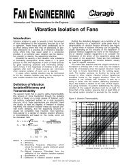
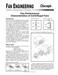
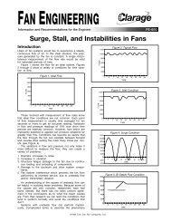
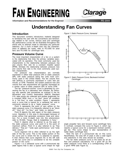
FAN ENGINEERINGInformation and Recommendations for the EngineerFE-2000Understanding Fan CurvesIntroductionThis document contains introductory material designedto familiarize the user with the conventions and terminologyrelated to fan curves. Various axial and centrifugalfan performance curves will be illustrated throughout thisarticle with no attempt made to rationalize any particularselection. For a more in-depth look into the characteristicsof different fan types, refer to FE-2300 for axialfans and FE-2400 for centrifugal fans.Pressure Volume CurveThe most important characteristic of a fan or a systemis the relationship that links the primary variables associatedwith its operation. The most commonly used fancharacteristic is the relationship between pressure riseand volume flow rate for a constant impeller speed(RPM). Similarly the relationship between pressure lossand volume flow rate is the most commonly used systemcharacteristic.Fan pressure rise characteristics are normallyexpressed in either total pressure (TP) or static pressure(SP), with static pressure being the units most commonlyused in the United States. The fan volume flowrate (airflow) is commonly expressed in cubic feet perminute, or CFM. Therefore, the system pressure loss andvolume flow rate requirements are typically expressed asa certain value of static pressure (SP) at some CFM.The fan “pressure-volume” curve is generated by connectingthe fan to a laboratory test chamber. By followingvery specific test procedures as outlined in the AirMovement and Control Association (AMCA) Standard210, data points are collected and plotted graphically fora constant RPM, from a “no flow” block off conditionto a “full flow” or wide condition. Figure 1 representssuch a curve that is typical for a vaneaxial fan, and iscommonly referred to as a “static pressure” curve.Point A represents the point of zero airflow on thestatic pressure curve. It is frequently referred to as “blockoff,” “shut off,” “no flow,” and “static no delivery.”Point B depicts the stall region of the static pressurecurve. Operation in this area is discouraged because oferratic airflow that generates excessive noise and vibration.For a more in-depth look into this phenomenonrefer to FE-600, “Surge, Stall & Instabilities in Fans.”Point C depicts what is referred to as the peak ofthe static pressure curve, and point D is the point ofmaximum airflow. Point D is also referred to as “freedelivery,” “free air,” “wide open performance,” and “wideopen volume.”Curve segment CD is often referred to as the rightside of the fan curve. This is the stable portion of thefan curve and is where the fan is selected to operate.It then follows that curve segment AC is the left sideof the fan curve and is considered to be the unstableportion of the curve.Figure 1 is a vaneaxial curve with a pronounced dip(stall region) that is also a typical curve shape for highFigure 1. Static Pressure Curve, VaneaxialSTATIC PRESSURE654321ABSTALLREGION0 0 1 2 3 4 5 6CFMFigure 2. Static Pressure Curve, Backward InclinedCentrifugalSTATIC PRESSURE76A54321BSTALL REGION0 0 1 2 3 4 5 6CFMCangle propeller fans and forward curve centrifugal fans.In contrast, compare this curve to Figure 2, which representsa typical curve for a backward inclined centrifugalfan. This curve shape is also representative ofradial blade centrifugal fans.Note the lack of a pronounced dip on this curve.Nevertheless, the area left of peak is also a stall regionand selections in this area should be avoided.The fan static pressure curve is the basis for all airflowand pressure calculations. For a given SP on thestatic pressure curve there is a corresponding CFM ata given RPM (see Figure 3).CRECOMMENDEDSELECTION RANGERECOMMENDEDSELECTION RANGEDD7 8 9©2001 Twin City Fan Companies, Ltd.

SPFigure 3. Static Pressure Curve, VaneaxialFigure 5. Static Pressure/Horsepower CurveBackward Inclined Centrifugal677566STATIC PRESSURE432STATIC PRESSURE543BHP543BHP1221SP10 0 1 2 3 4 5 6CFMSimply locate some unit of pressure on the left handSP scale and project a horizontal line to the point ofintersection on the static pressure curve. From the pointof intersection project a vertical line to the bottom CFMscale to establish the corresponding airflow at that particularspeed. In this example a static pressure of threeunits results in a CFM of 4.71 units.Brake Horsepower CurveHaving established a static pressure (SP) and an airflow(CFM), an operating brake horsepower (BHP) can beestablished (Figure 4).Figure 4. Static Pressure/Horsepower Curve, VaneaxialSTATIC PRESSURE6543BHP12108BHP60 0 1 2 3 4 5 6CFMEven though the performance curves for the vaneaxialfan and the centrifugal fan have completely differentshapes, the curves are read in the same way.Locate some unit of pressure on the left hand SP scale(4 units) and project a horizontal line to the point ofintersection with the SP curve. Projecting downwardfrom this point of intersection to the CFM scale weestablish an airflow of 6.55 units. Now project verticallyupward to intersect the BHP curve. Project a horizontalline from this point to the BHP scale and read a BHPof 6.86 units.Operating PointThe operating point (point of operation or design point)is defined as the fan pressure rise (SP)/volumetric flowrate (CFM) condition where the fan and system are in astable equilibrium. This corresponds to the condition atwhich the fan SP/CFM characteristic intersects the systempressure loss/flow rate characteristics.Figure 6 illustrates this fan/system operating point usingthe centrifugal fan performance curve from Figure 5.Figure 6. Fan/System Operating Point,Backward Inclined Centrifugal7 8 92477126600 1 2 3 4 5 6CFMBy adding the BHP curve to the static pressure curvefrom Figure 3 we complete the fan performance curve.To determine BHP simply extend vertically the CFMpoint established in Figure 3 until it intersects the BHPcurve. Draw a horizontal line from this point of intersectionto the right to the BHP scale to establish a BHP of7.27 units, which corresponds to the previously establishedperformance of 4.71 CFM units at 3.0 SP units.Similarly, we can add the BHP curve to the staticpressure curve of the backward inclined centrifugal fanfrom Figure 2 to complete that fan performance curve(Figure 5).2 Fan Engineering FE-2000STATIC PRESSURE543210 0 1 2 3 4 5 6CFMBHPSYSTEMLINEOPERATINGPOINTSP7 8 95432BHP1

The system line is simply a parabolic curve made upof all possible SP and CFM combinations within a givensystem and is determined from the fan law that SP variesas RPM 2 . Another fan law states that CFM varies asthe RPM. Therefore, we can also say that SP varies asCFM 2 . Note: Some systems have modulating damperswhich will not follow this parabolic curve.Sometimes a fan system does not operate properlyaccording to the design conditions. The measured airflowin the fan system may be deficient or it may bedelivering too much CFM. In either case, it is necessaryto either speed the fan up or slow it down to attaindesign conditions.Knowing that the fan must operate somewhere alongthe system curve, and knowing that it is possible topredict the fan performance at other speeds by applyingthe following fan laws:1. CFM varies as RPM2. SP varies as RPM 23. BHP varies as RPM 3We can now graphically present an “operating line”between various fan speeds using the fan/system operatingpoint data from Figure 6. This results in new SPcurves and BHP curves as shown in Figure 7.Figure 7. Variable Fan Characteristic Curve,Backward Inclined CentrifugalFigure 8. Variable System Characteristic Curve,Backward Inclined CentrifugalSP, FAN PRESSURE RISE – SYSTEM PRESSURE LOSS7654321{SYSTEMLINES0 0 1 2 3 4 5 6CFMCombining the fan control curve (Figure 7) with thesystem controlled curve (Figure 8) results in a fan/systemcontrolled curve having an “operating region” as shownin Figure 9.BHPOPERATINGLINESP7 8 9765432BHP1SP, FAN PRESSURE RISE – SYSTEM PRESSURE LOSS76543210 0 1 2 3 4 5 6CFMSPBHPSPINCREASINGRPMBHPSPBHPSYSTEMLINEOPERATINGLINEINCREASINGSPEED (RPM)7 8 97654321BHPFigure 9. Variable Fan/System Characteristic CurveBackward Inclined CentrifugalSP, FAN PRESSURE RISE – SYSTEM PRESSURE LOSS7654321{SYSTEMLINESFANCHARACTERISTICS{BHPOPERATINGREGIONSP7654321BHPThese speed changes represent an example of fancontrol that can be accomplished through drive changesor a variable speed motor.Another way to present an “operating line” is to adda damper, making the system the variable characteristic.By modulating the damper blades, new system lines arecreated resulting in an operating line along the fancurve. This can be seen graphically in Figure 8.0 0 1 2 3 4 5 6CFM7 8 9ConclusionThe foregoing methodology provides the knowledge necessaryto understand fan curves. When used in conjunctionwith FE-100, FE-600, FE-2300 and FE-2400, itprovides the user with the working knowledge necessaryto understand the fan performance characteristics andcapabilities of different fan equipment.3 Fan Engineering FE-2000

CLARAGE | www.CLARAGE.com2335 Columbia Highway | Pulaski, TN 38478 | Phone: 931-363-2667 | Fax: 931-363-3155