Chapter 6 Scaling Laws in Miniaturization
Chapter 6 Scaling Laws in Miniaturization
Chapter 6 Scaling Laws in Miniaturization

Create successful ePaper yourself
Turn your PDF publications into a flip-book with our unique Google optimized e-Paper software.
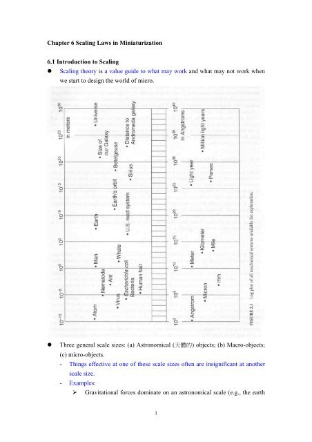
<strong>Chapter</strong> 6 <strong>Scal<strong>in</strong>g</strong> <strong>Laws</strong> <strong>in</strong> M<strong>in</strong>iaturization6.1 Introduction to <strong>Scal<strong>in</strong>g</strong>• <strong>Scal<strong>in</strong>g</strong> theory is a value guide to what may work and what may not work whenwe start to design the world of micro.• Three general scale sizes: (a) Astronomical ( 天 體 的 ) objects; (b) Macro-objects;(c) micro-objects.- Th<strong>in</strong>gs effective at one of these scale sizes often are <strong>in</strong>significant at anotherscale size.- Examples:‣ Gravitational forces dom<strong>in</strong>ate on an astronomical scale (e.g., the earth1
moves around the sun), but not on smaller scales.‣ Macro-sized motors use magnetic forces for actuation, but micro-sizedones usually use electrostatic fields <strong>in</strong>stead of magnetic.(Reference: MEMS Handbook, edited by Mohamed Gad-el-Hak, CRC Press)• Two types of scal<strong>in</strong>g laws:1. The first type: depends on the size of physical objects.2. The second type: <strong>in</strong>volves both the size and material properties of the system.6.2 <strong>Scal<strong>in</strong>g</strong> <strong>in</strong> Geometry• Surface and volume are two physical quantities that are frequently <strong>in</strong>volved <strong>in</strong>micro-device design.- Volume: related to the mass and weight of a device, which are related to bothmechanical and thermal <strong>in</strong>ertial.(thermal <strong>in</strong>ertial: related to the heat capacity of a solid, which is a measure ofhow fast we can heat or cool a solid. → important <strong>in</strong> design<strong>in</strong>g a thermalactuator)- Surface: related to pressure and the buoyant forces <strong>in</strong> fluid mechanics, aswell as heat absorption or dissipation by a solid <strong>in</strong> convective heat transfer.• Surface to volume ration (S/V ratio)2- S ∝ l ;3V ∝ l−1- S / V ∝ l- As the size l decreases, its S/V ratio <strong>in</strong>creases.- Examples‣ S/V ratio of an elephant (10 -4 ) vs. of a dragonfly (10 -1 )2
‣ An elephant and a flea have cells of about the same size. Too large acell will not have enough surface for substance exchanges with itssurround<strong>in</strong>gs to support the active metabolism ( 新 陳 代 謝 ) with<strong>in</strong>,unless it is highly elongated like a vertebrate nerve cell, <strong>in</strong>creas<strong>in</strong>g theS/V ratio. (Biochemistry by Mathews et al.)Figure 1.8: Range of sizes of objects studied by biochemists and biologists.(Biochemistry by Mathews et al.)Eukaryotes - Organisms whose cells are compartmentalized by <strong>in</strong>ternal cellular membranes to produce3
a nucleus and organelles.Lipids - 脂 質 , 脂6.3 <strong>Scal<strong>in</strong>g</strong> <strong>in</strong> Rigid-Body Dynamics6.3.1 <strong>Scal<strong>in</strong>g</strong> <strong>in</strong> Dynamic Forces1 s + at2= v20 t(6.3)By lett<strong>in</strong>g = 0 0,v22sa = (6.4)t2 sM3 2∝ ( l)(l )−2F = Ma =t(6.5)t6.3.2 The Trimmer Force <strong>Scal<strong>in</strong>g</strong> Vector• Trimmer (1989) proposed a unique matrix to represent force scal<strong>in</strong>g with relativeparameters of acceleration a, time t, and power density P/V 0 .• Force scal<strong>in</strong>g factor:F= [ lF⎡l⎢⎢l] =⎢l⎢⎣l1234⎤⎥⎥⎥⎥⎦(6.6)• Acceleration a: from Eq. (6.5),a = [ lF][ l]3 −1⎡l⎢⎢l=⎢l⎢⎣l1234⎤⎥⎥[l⎥⎥⎦−3⎡l⎢⎢l] =⎢ l⎢⎣ l−2−101⎤⎥⎥⎥⎥⎦(6.7)• Time t: from Eq. (6.5),t =2sMF1∝ ([ l ][ l3][ l−F])0.5⎡l⎢⎢ l=⎢l⎢⎣ l1.510.50⎤⎥⎥⎥⎥⎦(6.8)4
• Power Density P/V 0 : from Eq. (6.5),W F ⋅ sS<strong>in</strong>ce P = = , thust tP Fs = (6.9)V0tV 0⇒PV=([ l[ l][ l1 3 −F0.5 30][ l ][ l ]) [ l ]F1]−⎡l⎢⎢ l=⎢ l⎢⎣ l2.5−10.52⎤⎥⎥⎥⎥⎦(6.10)6.4 <strong>Scal<strong>in</strong>g</strong> <strong>in</strong> Electrostatic Forces• In Fig. 6.4, the electric potential energy <strong>in</strong>duced <strong>in</strong> the parallel plates is:U1CV2ε rε WL2d20 2= − = − V(2.7)• Breakdown voltage- The voltage required to <strong>in</strong>itiate discharge.1- For d > 10µm , V ∝ l (see Fig. 6.5)5
( l)( l)( l )( ll)( l)0 0 1 1 1 23⇒ U ∝= l(6.11)1- A factor of 10 decrease <strong>in</strong> l<strong>in</strong>ear dimension will decrease the potentialenergy by a factor of 1000.• In Fig. 6.6, the electrostatic forces are,FFF∂U∂d- F , F , and F ∝ ( l21 ε ε WLV2 d2r 0d= − = −(2.8)2WL2∂U1 εrε0LV= − =∂W2 d(2.10)2∂U1 εrε0WV= − =∂L2 d(2.11)d W L)- A 10 times reduction <strong>in</strong> the plate sizes means a 100 times decrease <strong>in</strong>the <strong>in</strong>duced electrostatic forces.6.5 <strong>Scal<strong>in</strong>g</strong> <strong>in</strong> Electromagnetic Forces• In this section, it is shown that electromagnetic actuation is not scaled down6
nearly as favorably as electrostatic forces.- The electromagnetic forces can be <strong>in</strong>duced <strong>in</strong> a conductor or aconduct<strong>in</strong>g loop <strong>in</strong> a magnetic field B by pass<strong>in</strong>g current i <strong>in</strong> theconductor.- The electromotive force (emf) is the force that drives the electrons-through the conductor.21 φU = (6.13)2 Lwhere φ is the magnetic flux, and L is the <strong>in</strong>ductance.- S<strong>in</strong>ce φ = Li ,1 Li2U =2(6.14)- The <strong>in</strong>duced electromagnetic force would be∂UF =∂x- For constant current case,φ=cons tan ti=cons tan t(6.15a)∂UF = (6.15b)∂x1F = i22∂L∂x20S<strong>in</strong>ce i ∝ l and ∂L/ ∂x∝ l ,4F ∝ l- If 10 times reduction <strong>in</strong> size (l)⇒ Electromagnetic force: 10,000 times reductionComparison: Electrostatic force: only 100 times reductionConclusion: Electromagnetic force is less favorable <strong>in</strong> scale-down thanElectromagnetic force.6.6 <strong>Scal<strong>in</strong>g</strong> <strong>in</strong> Electricity• Examples: Microsystem actuation by electrostatic, piezoelectric, and thermalresistance heat<strong>in</strong>g.• Electric Resistance:LA−1R = ρ ∝ l(6.18)where ρ, L, and A are the resistivity, length, and cross-sectional area, respectively.• Electric Power Loss:PVR21= ∝ l(6.19)7
where V is the applied voltage ∝ l0• Electric field energy density:1 2 −2u = ε E ∝ l(6.20)20−1where the dielectric permittivity ε ∝ l , and the electric field E ∝ l .3• Example: For a system that carries its own power, the available power E av ∝ l .P −2⇒ ∝ l . (6.21)Eav- That is, a 10 times reduction of l leads to 100 times greater power lossdue to the resistance <strong>in</strong>crease.- Disadvantage of scal<strong>in</strong>g down of power supply systems.6.7 <strong>Scal<strong>in</strong>g</strong> <strong>in</strong> Fluid Mechanics• In Fig. 6.7, mov<strong>in</strong>g the top plate to the right <strong>in</strong>duces the motion of the fluid.- Newtonian flow:dθτ ∝ , ordtdθdVτ = µ = µdt dywhere τ: shear stress; μ: coefficient of viscosity ( 黏 滯 性 ); dθ/dt:stra<strong>in</strong> rate; V: fluid velocity.-τThus, µ =R s(6.22)where R s =V max /h- Rate of volumetric fluid flow: Q =A s V ave (6.23)where A s : cross-sectional area for the flow; V ave : average velocity ofthe fluid.8
• Renolds number:ρVLRe =µwhere ρ: fluid density; V & L: characteristic velocity and length scales of theflow.- Re ∝ (<strong>in</strong>ertial forces)/(viscous force)- Macro flows: high <strong>in</strong>ertial forces → high Re → turbulence flow- Micro flows: high viscosity → low Re → lam<strong>in</strong>ar flowp.s.: (1) turbulence flow: fluctuat<strong>in</strong>g and agitated;(2) lam<strong>in</strong>ar flow: smooth and steady;(3) transition from lam<strong>in</strong>ar to turbulent: 10 3 ~10 5(from “Micromach<strong>in</strong>es: A New Era <strong>in</strong> Mechanical Eng<strong>in</strong>eer<strong>in</strong>g,” by Iwao Fujimasa,Oxford University Press, 1996)• In Fig. 6.8, with the pressure drop ΔP over the length L, the rate of volumetricflow of the fluid is (Hagen-Poiseuille law),πa4 ∆PQ = (6.24)8µL9
Q- With V = aveπ2a, 8µVaveL∆ P =(6.25)a24- Thus, Q ∝ a ;∆P∝ aL−26.8 <strong>Scal<strong>in</strong>g</strong> <strong>in</strong> Heat Transfer6.8.1 <strong>Scal<strong>in</strong>g</strong> <strong>in</strong> Heat Conduction ( 傳 導 )<strong>Scal<strong>in</strong>g</strong> of Heat Flux• Heat conduction <strong>in</strong> solid is governed by the Fourier law,∂T( x,y,z,t)‣ q x= −k∂xwhere q x : heat flux along the x axis; k: thermal conductivity of thesolid; T(x,y,z,t): temperature field.‣ Rate of heat conduction:‣ For solids <strong>in</strong> meso- and microscales,2 −11( l )( l ) lQ ∝ =∆TQ = qA = −kA(6.27)∆xThat is, reduction <strong>in</strong> size leads to the decrease of total heat flow.<strong>Scal<strong>in</strong>g</strong> <strong>in</strong> Submicrometer Regime• In the submicrometer regime, the thermal conductivity is,k131= cVλ ∝ l(6.28)where c, V, and λ are specific heat, molecular velocity, and average mean freepath, respectively.1 1 2- Thus, Q ∝ ( l )( l ) = l(6.29)- A reduction <strong>in</strong> size of 10 would lead to a reduction of total heat flowby 100.10
<strong>Scal<strong>in</strong>g</strong> <strong>in</strong> Effect of Heat Conduction <strong>in</strong> Solids of Meso- and Micro-scales• A dimensionless number, called the Fourier number, F 0 is used to determ<strong>in</strong>e thetime <strong>in</strong>crements <strong>in</strong> a transient heat conduction analysis.αtL- F0=2where α: thermal diffusivity of the material, and t: time for heat toflow across the characteristic length L.F- t = L α0 2 2∝ l6.8.2 <strong>Scal<strong>in</strong>g</strong> <strong>in</strong> Heat Convection ( 對 流 )• Heat transfer <strong>in</strong> fluid is <strong>in</strong> the mode of convection (Newton’s cool<strong>in</strong>g law),Q = qA = hA∆T(6.32)where Q: total heat flow between two plates; q: heat flux; A: cross-sectional area forthe heat flow; h: heat transfer coefficient;two po<strong>in</strong>ts.∆ T: temperature difference between these- h: depends primarily on the fluid velocity, which does not play asignificant role <strong>in</strong> the scal<strong>in</strong>g of the heat flow.- Thus, <strong>in</strong> meso- and micro-regimes,Q ∝ A ∝ l2• For the cases <strong>in</strong> which gases pass <strong>in</strong> narrow channels at submicro-meter scale,‣ The classical heat transfer theories based on cont<strong>in</strong>uum fluids breakdown.‣ The seem<strong>in</strong>gly convective heat transfer has <strong>in</strong> fact become conductionof heat among the gas molecules as the effect of the boundary layerbecomes a dom<strong>in</strong>ant factor.‣ In Fig. 6.9, H < 7λwhere λ =65nm for gases, and 1.3 μm for liquids.11
1‣ λ ∝ρ1‣ k = cVλ3‣ V =8kTπmwhere T: mean temperature of the gas; and m: molecular weight of thegas.‣ Effective heat flux:k∆Tq eff= (6.34)H + 2εwhere ∆ T : temperature difference between two plates; ε: depends on thegases entrapped between two plates, 2.4λ