- Page 3 and 4: CIICT 2009Proceedings of the China-
- Page 5 and 6: ForewordOn behalf of the organising
- Page 7 and 8: TABLE OF CONTENTSSection 1A: ANTENN
- Page 9 and 10: Section 3B: COMPUTER VISION 133A ne
- Page 11 and 12: Section 1AANTENNAS AND CIRCUITS 11
- Page 13 and 14: A block diagram of the platform is
- Page 15 and 16: These two paths are averaged to red
- Page 18 and 19: 4 mm -10 0 , -8 0 , -3 mm -8 0 , -6
- Page 20 and 21: The results show that the separatio
- Page 22 and 23: same size of annular-ring outer rad
- Page 25 and 26: [4] C.Y.Sim, K.W.Lin, J.S.Row, Desi
- Page 27 and 28: Interpretation of Spatial Movement
- Page 30 and 31: III.DATA COLLECTIONAccurate spatial
- Page 32 and 33: navigation. We define a walking are
- Page 34 and 35: one’s body position, movement and
- Page 36 and 37: world and will result in them being
- Page 38 and 39: GPS/RFID/Self-contained Sensor Syst
- Page 40 and 41: When the headway measures are equal
- Page 42 and 43: [4] R.Liu, and S. Sinha, “Modelli
- Page 44 and 45: Digital Audio Watermarking by Magni
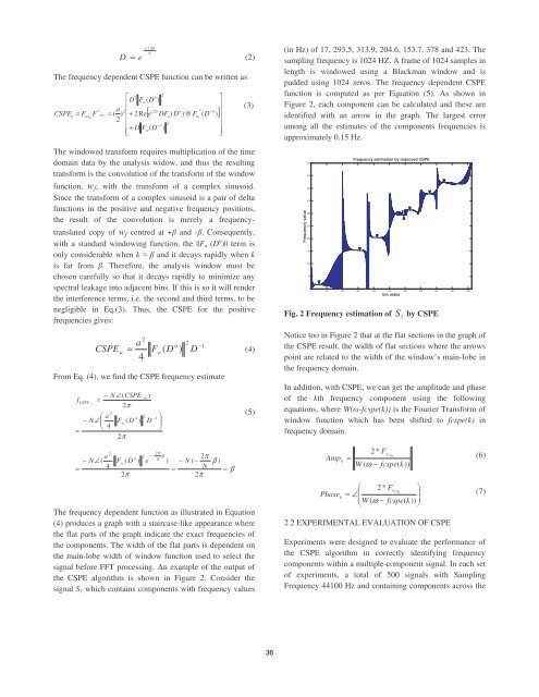
- Page 48 and 49: accurate in identifying the compone
- Page 50 and 51: Furthermore, the decode experiment
- Page 52 and 53: exists no spatial information of th
- Page 54 and 55: iteration, one NMF for each frame.
- Page 56 and 57: 7. CONCLUSIONSIn this paper we empl
- Page 58 and 59: Dej 2 πβN= (1)The frequency depen
- Page 60 and 61: length of x 1[n ], while it only ap
- Page 62 and 63: Computing Modified Bessel functions
- Page 64 and 65: From (9) both the numerator and den
- Page 66 and 67: Section 2ARADIO SYSTEMS 156
- Page 68 and 69: puncturing some parity RSDT columns
- Page 70 and 71: [5] O'Droma M. S. and I. Ganchev.
- Page 72 and 73: Administrations (CEPT) has proposed
- Page 74 and 75: Figure 3 Proposed Test PlatformThe
- Page 76 and 77: ACKNOWLEDGEMENTSThe authors wish to
- Page 78 and 79: in an optimal fashion within that e
- Page 80 and 81: whether the agent is in a learning
- Page 82 and 83: needs of the experiments as the goa
- Page 84 and 85: Section 2BGEOCOMPUTATION74
- Page 86 and 87: describes the proposal put forward
- Page 88 and 89: However, individual sensor measurem
- Page 90 and 91: Position Of Test Phone CallPosition
- Page 92 and 93: vol. 6, no. 3, pp. 30-38, 2007.[11]
- Page 94 and 95: environment’. The report states t
- Page 96 and 97:
awareness communications about Twit
- Page 98 and 99:
2.2 Flight route planningFlight rou
- Page 100 and 101:
Spatial - temporal Simulation and P
- Page 102 and 103:
and serious ones in turn. Overall,
- Page 104 and 105:
[3] Cheng Weiming, Zhou Chenghu, an
- Page 106 and 107:
(a) 1973 (b) 1990 (c) 2000Figure 1.
- Page 108 and 109:
Effect of Hard RTOS on DPDC SCADA S
- Page 110 and 111:
Therefore, this solution is not fea
- Page 112 and 113:
already done on error free system o
- Page 114 and 115:
8 PROPOSED REAL-TIME OPERATING SYST
- Page 116 and 117:
HYBRID DECODING SCHEMES FOR TURBO-C
- Page 118 and 119:
L a(u k ) SOVA/Log-MAPLog-MAP Inter
- Page 120 and 121:
JavaScript code Fragment Analyzingf
- Page 122 and 123:
The external JavaScript itself, whi
- Page 124 and 125:
Section 3ACHANNELS AND PROPAGATION1
- Page 126 and 127:
The DCF is assumed to have negligib
- Page 128 and 129:
When m=6, the fluctuation have been
- Page 130 and 131:
Across a 5 MHz spectrum, the maximu
- Page 132 and 133:
Fig 6 shows the time variant charac
- Page 134 and 135:
In the system, the RF signal is dir
- Page 136 and 137:
of the different speeds UWB standar
- Page 138 and 139:
3dB higher for the laser biased at
- Page 140 and 141:
information for inter domain pre-au
- Page 142 and 143:
In addition, the opendiameter imple
- Page 144 and 145:
A new algorithm of edge detection b
- Page 146 and 147:
Control structure elements of shape
- Page 148 and 149:
3D TOOTH RECONSTRUCTIONWITH MULTIPL
- Page 150 and 151:
3.1 Topological structure and base
- Page 152 and 153:
Automatic Recognition of Head Movem
- Page 154 and 155:
threshold model λ is created to ca
- Page 156 and 157:
Dirt and Sparkle Detection for Film
- Page 158 and 159:
[4] T. Komatsu, T. Saito, “Detect
- Page 160 and 161:
Lightweight Signal Processing Algor
- Page 162 and 163:
a two element PIR sensor, to obtain
- Page 164 and 165:
the sensor node can readily be chec
- Page 166 and 167:
parameters may not lead to simple a
- Page 168 and 169:
0 (1 dR1)(1 dR2) 1[1]where d is t
- Page 170 and 171:
epeatability is normally defined as
- Page 172 and 173:
Integrated air quality monitoring:
- Page 174 and 175:
colour coded data that are used to
- Page 176 and 177:
Approximate Analysis of Fibre Delay
- Page 178 and 179:
Virtual Traffic SourceA*f( t)= A* e
- Page 180 and 181:
Section 4AANTENNAS AND CIRCUITS 217
- Page 182 and 183:
Primary SpiralSecondary SpiralCoCbL
- Page 184 and 185:
[4] A H Miklich, J X Przybysz, T J
- Page 186 and 187:
ased on the ABCD transmission matri
- Page 188 and 189:
RRe( Y3 _ LowFreq)=s(19)2 2 2Rs+ ω
- Page 190 and 191:
Section 4BeLearning180
- Page 192 and 193:
were investigated as important inpu
- Page 194 and 195:
Time [min]1009080706050403020100Loc
- Page 196 and 197:
Mean Rating for Different Encoding
- Page 198 and 199:
Billing Issues when Accessing Perso
- Page 200 and 201:
data consumed, for example 0.2€/M
- Page 202 and 203:
and returns billing plans the learn
- Page 204 and 205:
lecture size and the price per quan
- Page 206 and 207:
Section 5ARADIO SYSTEMS 2196
- Page 208 and 209:
and is uniformly distributed in the
- Page 210 and 211:
When the number of users is 2, and
- Page 212 and 213:
III.BLUETOOTH OPERATIONS IN SNIFF M
- Page 214 and 215:
traffic or for POLL and NULL packet
- Page 216 and 217:
Necessity for an Intelligent Bandwi
- Page 218 and 219:
Spruce: Spruce has been one of the
- Page 220 and 221:
Fig. 5 Comparison of bandwidth calc
- Page 222 and 223:
Section 5BCOMPUTER NETWORKS 2212
- Page 224 and 225:
2.1 CNFThe Content Navigating Funct
- Page 226 and 227:
User BGF PD-FE CSCF CNF(AS) HSSPeer
- Page 228 and 229:
5 ConclusionThis paper proposed an
- Page 230 and 231:
d( X − X ) + ( Y −Y)= ∑ ∑2
- Page 232 and 233:
Program Dependence Graph Generation
- Page 234 and 235:
CDGPDGFigure 2. Program Dependence
- Page 236 and 237:
Section 6ADIGITAL HOLOGRAPHY226
- Page 238 and 239:
away. Immediately behind this plane
- Page 240 and 241:
While this is not ideal as hair is
- Page 242 and 243:
Figure 12. 3-D visualisation of 200
- Page 244 and 245:
Speed up of Fresnel transforms for
- Page 246 and 247:
[9]L. Onural and H. Ozaktas, "Signa
- Page 248 and 249:
2009 China-Ireland International Co
- Page 250 and 251:
2009 China-Ireland International Co
- Page 252 and 253:
that enables the complete separatio
- Page 254 and 255:
developed in the literature to remo
- Page 256 and 257:
Section 6BINTELLIGENT SYSTEMS246
- Page 258 and 259:
the vectors remain just form the in
- Page 260 and 261:
d d x,y . If x and y don’t belon
- Page 262 and 263:
Investigating the Influence of Popu
- Page 264 and 265:
TABLE I.EXPERIMENTAL RESULTS FOR 26
- Page 266 and 267:
Intelligent Learning Systems Where
- Page 268 and 269:
FuzzyLogicBayesianReasoningClassifi
- Page 270 and 271:
AN IMPROVED HAPTIC ALGORITHM FOR VI
- Page 272 and 273:
Fig. 2. Proxy ImmersionFig. 1. Prox
- Page 274 and 275:
1Corpus Design Techniques for Irish