A Data Streaming Algorithm for Estimating Entropies of OD Flows

A Data Streaming Algorithm for EstimatingEntropies of OD FlowsHaiquan (Chuck) ZhaoGeorgia Inst. of TechnologyOliver SpatscheckAT&T Labs – ResearchAshwin LallUniversity of RochesterJia WangAT&T Labs – ResearchMitsunori OgiharaUniversity of RochesterJun (Jim) Xu ∗Georgia Inst. of TechnologyABSTRACTEntropy has recently gained considerable significance as animportant metric for network measurement. Previous researchhas shown its utility in clustering traffic and detectingtraffic anomalies. While measuring the entropy of thetraffic observed at a single point has already been studied,an interesting open problem is to measure the entropy of thetraffic between every origin-destination pair. In this paper,we propose the first solution to this challenging problem.Our sketch builds upon and extends the L p sketch of Indykwith significant additional innovations. We present calculationsshowing that our data streaming algorithm is feasiblefor high link speeds using commodity CPU/memory at areasonable cost. Our algorithm is shown to be very accuratein practice via simulations, using traffic traces collectedat a tier-1 ISP backbone link.Categories and Subject DescriptorsC.2.3 [Computer-Communication Networks]: NetworkOperations—Network MonitoringGeneral TermsAlgorithms, Measurement, TheoryKeywordsNetwork Measurement, Entropy Estimation, Data Streaming,Traffic Matrix, Stable Distributions1. INTRODUCTIONThe (empirical) entropy of the network traffic has recentlybeen proposed, in many different contexts, as an effective∗ Supported in part by NSF grants CNS 0716423, CNS0626979, CNS 0519745, and NSF CAREER award CNS0238315.Permission to make digital or hard copies of all or part of this work forpersonal or classroom use is granted without fee provided that copies arenot made or distributed for profit or commercial advantage and that copiesbear this notice and the full citation on the first page. To copy otherwise, torepublish, to post on servers or to redistribute to lists, requires prior specificpermission and/or a fee.IMC’07, October 24-26, 2007, San Diego, California, USA.Copyright 2007 ACM 978-1-59593-908-1/07/0010 ...$5.00.and reliable metric for anomaly detection and network diagnosis[3, 11, 15, 24, 25]. Measuring this quantity exactly inreal time (say by maintaining per-flow states), however, isnot possible on high-speed links due to its prohibitively highcomputational and memory requirements. For this reason,various data streaming algorithms [16] have been proposedto approximate this quantity. Data streaming [19] is concernedwith processing a long stream of data items in onepass using a small working memory (called a sketch) in orderto answer a class of queries regarding the stream. Thechallenge is to use this sketch to “remember” as much informationpertinent to our problem as possible.We observe that it is often important to know the entropiesof origin-destination (OD) flows, where an OD flowis defined as all the traffic that enters an ingress point (calledorigin) and exits at an egress point (called destination).Knowing these quantities will give us significantly more insightinto the dynamics of traffic inside an ISP network,which we will elaborate upon shortly. However, we foundthat none of the existing entropy estimation algorithms [1,2, 5, 16] can be extended to solve this new problem. In particular,the traffic matrix estimation literature [18, 21, 22,23, 27] has ruled out the following naive approach: separatethe traffic at each ingress point into various OD flowsin real time and feed them to existing entropy estimationalgorithms. In this paper, we propose the first solution tothis new problem.1.1 MotivationThe ability to estimate entropy for all OD flows in a networkcan be highly beneficial. On today’s Internet, networkperformance degradation and service disruption canbe caused by a wide range of events, including anomalies(e.g., DDoS attacks, network failures, and flash crowds) andscheduled network maintenance tasks (e.g., router IOS updatesand customer migration). Many of these events occurin a distributed manner (intentionally or unintentionally)in terms of their signatures and impacts. Detecting theseevents and evaluating their impact on network services thusoften requires monitoring of the traffic from a number of locationsacross the network. More importantly, these changesin traffic distribution may be totally invisible in the traditionaltraffic volume matrix. However, by examining theentropy of every OD flow in the network, one can hope tocapture these events in real time.To illustrate how beneficial the OD flow entropy estimationis, consider a situation in which a link fails (e.g., due to

hardware problems) and is cost out for maintenance. Thetraffic flows that used to be carried on that link will mostlikely be redistributed to alternative paths. In the very rarecase where no alternative path exists or the network experienceslong convergence delay, the flows may abort completely.In either case, traffic distribution on a number oflinks across the network will change. It is possible that thetraffic volume changes on those impacted links are small,and sometimes too small to be detected on each link usingvolume based detection algorithms. However, the overallchange in the traffic distribution across the network can bequite large. If so, the examination of traffic entropy alongwith the traffic matrix for all OD flows is likely to enableus to capture such distributed and dynamically occurringevents.Another example is a DoS attack. When there is a distributedDoS attack launched from outside the network, itsimpact may not be immediately visible in the traffic matrixin terms of traffic volume change. However, it is very importantfor operators to be able to detect and mitigate theattack at the earliest time to minimize the possible negativeimpact on their services. That is, it may be too latefor certain types of events to be detected when their impactbecomes visible in the traffic volume matrix. In addition,certain types of DoS attacks are difficult to detect due tothe low-rate nature of attack flows [14, 26]. In such cases,we hope to be able to achieve real time detection based ontraffic entropy estimation.1.2 Our solution and contributionsIn this work, we propose the first solution to the challengingproblem of estimating the entropies of all OD flows.Our key innovation is to invent a sketch that allows us toapproximately estimate not only (a) the entropy of a datastream, but also (b) the entropy of the intersection of twodata streams A and B from the sketches of A and B. We referto property (b) as the “intersection measurable property”(IMP) in the sequel. Note that all existing entropy estimationalgorithms (their sketches) have property (a), but noneof them has IMP.The intersection measurable property (IMP) of our sketchleads to the following very elegant solution of our problem.Each participating ingress and egress node in the networkmaintains a sketch of the traffic that flows in/out of it duringa measurement interval. When we would like to measure theentropy of an OD flow stream between an ingress point i andan egress point j, we simply summon from node i the sketchof its ingress stream O i, and from node j the sketch of itsegress stream D j, and then infer the entropy of O i ∩ D jusing the sketches’ IMP. This solution is extremely costeffectivein that we will be able to estimate O(k 2 ) quantities(the entropies of a k by k OD flow stream matrix) usingonly O(k) sketches. However sketches that have IMP aremuch harder to design than those without it, and hence thesignificant challenge we have in this work.Our sketch builds upon and extends the L p sketch of Indyk[12] with significant additional innovations. Indyk’ssketch was designed for the estimation of the L p norm ofa stream (defined later). We observe that Indyk’s L p sketchhas the desirable IMP, and therefore allows for the estimationof the L p norm of an OD flow O i ∩ D j using the L psketches at O i and D j. However, we have to develop theIMP theory of L p sketch ourselves since IMP was never evenclaimed in [13] (probably because there was no applicationin sight for IMP at that time).Our most important contribution is to discover that theentropy of an OD flow can be approximated by a functionof just two L p norms (L p1 and L p2 , p 1 ≠ p 2) of the ODflow. With this insight, our sketch at each ingress and egresspoint is simply one L p1 sketch and one L p2 sketch. In thisway, we not only solve this difficult problem, but also find anice application for the L p sketch. From a theoretical pointof view, our solution resolves one of the open questions ofCormode [7].Our contributions can be summarized as follows. First,our discovery builds a mathematical connection between ourproblem and Indyk’s L p norm estimation problem, leadingto a highly cost-effective solution. Second, we extend Indyk’s(ɛ, δ) analysis of L p sketches [13] using asymptotic normalityof order statistics, leading to much tighter (yet slightlyless rigorous) accuracy bounds. We also modify Indyk’s algorithmto make it run fast enough for processing traffic atvery high-speed links (e.g., 10 million packets per second).Finally, we thoroughly evaluate the accuracy of our solutionby simulating it on real-world packet traces collected at atier-1 ISP backbone. We show that our algorithm deliversvery accurate estimations of the OD flow entropies.The remainder of this paper is organized as follows. InSection 2 we give a high-level overview of how the differentcomponents of our entire scheme works. In Section 3through 6 we describe the major components of our algorithm.• In Section 3 we introduce stable distributions and describeIndyk’s algorithm to estimate the L p norm usingthem.• In Section 4 we show how to estimate entropy from L pnorm.• In Section 5 we show the intersection measurable property(IMP) of the L p norm algorithm.• In Section 6 we modify the L p norm algorithm to improveits accuracy under tight resource constraints.In Section 7 we discuss the hardware implementation ofour algorithm. In Section 8 we demonstrate the accuracyof our algorithm via simulations run on real-world data. InSection 9 we briefly survey previous work that is related toours. Finally, we conclude in Section 10. The Appendixcontains the proof of some of the theorems.2. PROBLEM STATEMENT AND OVERVIEWIn this section, we describe precisely the problem of estimatingthe entropies of OD flows and offer an overview ofour solution approach. As defined before in [16], given astream S of packets that contains n (transport-layer) flowswith sizes (number of packets) a 1, a 2, ..., a n respectively,its empirical entropy H(S) is defined as − P n a ii=1 slog 2 ( a is),where s = P ni=1ai is the total number of packets in S.1We have shown before [16] that to estimate the empirical1 Throughout this paper logarithms will be base e except inthe definition of empirical entropy here. Since the logarithmbase e and the logarithm base 2 are different by a constantmultiplicative factor, it does not affect our analysis of relativeerrors.

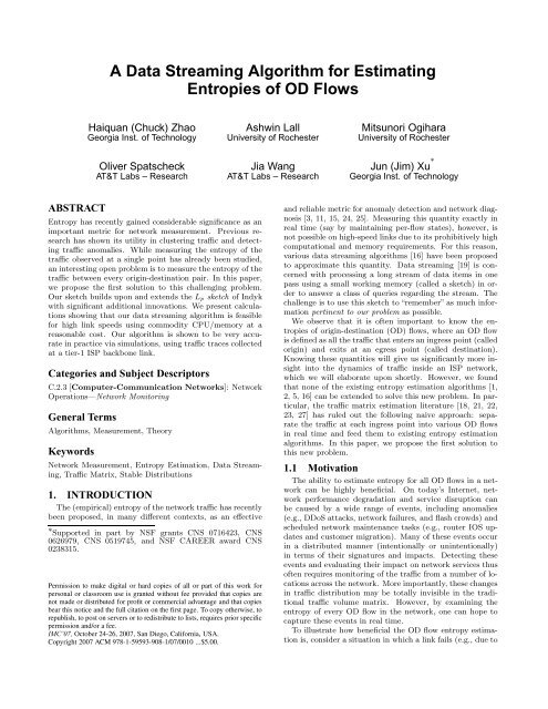
entropy of a stream S, it suffices to to estimate a relatedquantity called entropy norm ||S|| H, defined as P iai ln (ai),since H(S) can be rewritten asH(S) = − X a“is log ai”2si= log 2 (e)[ln (s) − 1 Xa i ln (a i)],sand s is usually a known quantity.The entropy of an OD flow stream OD ij between an ingresspoint i and an egress point j, is definedTas the entropy oftheir intersection, i.e., H(OD ij) ≡ H(O i Dj). To derivethis entropy value from the above formula,Thowever, we needto measure both the entropy norm ||O iT Dj|| H and s in orderto compute the entropy of H(O i Dj). Note that inour case, s is the volume of the OD flow and is an unknownquantity that needs to be estimated/inferred separately. Asdescribed in Section 1.2 , our solution is to invent a sketchfor estimating the entropy norm of a stream that has theintersection measurable property (IMP).Our algorithm and sketch build upon Indyk’s classical resultson estimating the L p norm of a stream using the theoryof stable distributions, for values of p in (0, 2]. In [13], Indykpresents an algorithm for computing the L p norm ofa stream S. For a stream S that contains n flows of sizesa 1, . . . , a n, its L p norm ||S|| p is defined as ( P i |ai|p ) 1/p , so||S|| p p = P i |ai|p . We discover that the data streaming solutionof Indyk has the aforementioned IMP. Interestingly,this nice intersection property was never claimed in [13] oranywhere else. We will develop an entropy estimation techniquethat fully takes advantage of this property and offerits rigorous analysis.While the work of Indyk is very influential, the practicalimportance of being able to estimate the L p norm forvalues other than 1 and 2 was never clear. In our work,the L p norms for p values slightly above or below 1 playa crucial role as follows. On realizing that Indyk’s algorithmcan be extended for estimating the L p norms of anOD flow, we came up with the wild conjecture that it ispossible to approximate the function x ln(x) using a linearcombination of a small number of functions in the family{x p |p ∈ (0, 2]}. In other words, we conjectured that we canfind parameters c 1, . . . , c k ∈ R and p 1, . . . , p k ∈ (0, 2] suchthat x ln(x) ≈ P kj=1 cj ∗ xp j. If this conjecture is true, thenwe will be able to estimate the entropy norm of an OD flowstream S as P kj=1 cj ∗ ||S||p jp j, where ||S|| pj , j = 1, . . . , k canbe estimated using our extension of Indyk’s algorithm forstream intersection. We emphasize that it took a leap offaith for us to think in this direction, as most of the approximationschemes we encountered in mathematical literatureare by linear combination of terms like x j (approximationby polynomial) and sin(x) (Fourier expansion).Our wild conjecture has been proven correct! To ouramazement we found that by using a linear combination of1only two functions in the family, in the form of2α (x1+α −x 1−α ), we can approximate x ln(x) very closely for all x valuesin a large interval, e.g., [1, 1000] or [1, 5000]. Here α is atunable parameter that takes small values. For example, inFigure 1, we show how closely we can approximate x ln(x)using 10(x 1.05 − x 0.95 ) within the interval [1, 1000]. In otherwords, if all transport-layer flows in an OD flow S have lessthan 1000 packets, we can estimate the entropy norm of thei800070006000500040003000200010000approximationy = xln(x)0 100 200 300 400 500 600 700 800 9001000Figure 1: Comparison of entropy function and theapproximationOD flow as 10(||S|| 1.051.05 − ||S|| 0.950.95). It turns out that this“symmetry” of the exponents (1 + α and 1 − α) around 1serves another very important purpose that we will describeshortly.We found that the approximation becomes gradually worsewhen x becomes larger than 1000 (packets), but the relativeerror level is generally acceptable up until 5000. Therefore, ifthere are some very large transport-layer flows (say with tensof or hundreds of thousands of packets) inside an OD flow S,the estimation formula such as 10(||S|| 1.051.05 − ||S|| 0.95) 0.95 maydeviate significantly from its entropy norm. Fortunately,identifying such very large flows is a well-studied problemin both computer networking (e.g., [10]) and theory (e.g.,[17]). We will adopt the “sample and hold” algorithm proposedin [10] to identify all flows that are much larger thana certain threshold (say 1000 packets) and compute theircontributions to the OD flow entropy separately.Now the last piece of the puzzle is that when we computethe entropy H from the entropy norm, we need to knows, the total volume of the OD flow. Estimating this volumeis a task known as traffic matrix estimation [18, 21,22, 23, 27]. Various techniques for estimating the trafficmatrix have been proposed that are based on statistical inferenceor direct measurement (including data streaming).In fact, this quantity is exactly the L 1 norm, which canbe estimated using Indyk’s L 1 norm estimation algorithmwith IMP extensions. It turns out that we need none ofthese. Recall that our approximation formula is in the form1of2α (x1+α −x 1−α ), where α is a small number such as 0.05.We observe that, in this case, the function x can indeed beapproximated by (x 1+α +x 1−α )/2 and therefore the OD flowvolume (i.e., the L 1 norm) can be approximated by the averageof ||S|| 1+α1+α and ||S||1−αcalculated from the OD flow.Therefore, our sketch data structure allows us to kill twobirds (the L 1 norm and the entropy norm) with one stone!3. PRELIMINARIESFor the purposes of this paper we define a flow to be allthe packets with the same five-tuple in their headers: sourceaddress, destination address, source port, destination port,and protocol.Clearly, we will not be able to compute the entropy ofeach distribution exactly, so we use the following type ofapproximation scheme. An (ɛ, δ) approximation scheme isone that returns an approximation ˆθ for a value θ such that,with probability at least 1−δ, we have (1−ɛ)θ ≤ ˆθ ≤ (1+ɛ)θ.

has distribution S(p). Note that, due to the symmetry ofS(p), DMed p is exactly the three-quarter quantile of S(p).Although there is no closed form for DMed p for most of thep values, we can numerically calculate it by simulation, orwe can use a program like [20].Intuitively, the correctness of this estimator can be justifiedas follows. Since Y 1/||S|| p, ..., Y l /||S|| p are i.i.d. randomvariables with distribution S(p), taking absolute value givesus i.i.d. draws from S + (p). For large enough l, their medianshould be close to the distribution median of S + (p). Therefore,we simply divide median(|Y 1|, . . . , |Y l |) by the distributionmedian of S + (p) to get an estimator of ||S|| p. We haveto take absolute values because the distribution median ofS(p) is 0 due to its symmetry. In the next section we willanalyze the relative error of this estimator.Indyk’s estimator for the L p norm is based on the propertyof the median. We find, however, that it is possible toconstruct estimators based on other quantiles and they mayeven outperform the median estimator, in terms of estimationaccuracy. However, since the improvement is marginalfor our parameters settings, we stick to the median estimator.3.3 Error analysis for L p norm estimatorIn this section we analyze the performance of the estimatorfor ||S|| p in (1).3.3.1 (ɛ, δ) bound for p = 1Here we basically restate Lemma 2 and Theorem 3 fromIndyk [13] with the constants spelled out. We arrived atthis by using Chernoff bounds to derive the constant in hisClaim 2.Theorem 1. (Indyk, [13]) Let ⃗ X = (X 1, . . . , X l ) be i.i.d.samples from S(1), l = 8(ln 2 + ln 1 δ )/ɛ2 , ɛ < 0.2, thenDMed 1 = 1, and P r[median(|X 1|, . . . , |X l |) ∈ [1−ɛ, 1+ɛ]] >1 − δ. Thus (1) gives an (ɛ, δ) estimator for p = 1.Example: for p = 1, δ = 0.05, ɛ = 0.1, we get l = 2951.This is a very loose bound in the sense that we need a verylarge l. This motivates us to resort to the asymptotic normalityof the median for some approximate analysis.3.3.2 Asymptotic (ɛ, δ) bound for p ∈ (0, 2]z δ/22mf(m)ɛ )2 ,Theorem 2. Let f = f S + (p), m = DMed p, l = (then (1) gives an estimator with asymptotic (ɛ, δ) bound. z ais the number such that for standard normal distribution Zwe have P r[Z > z a] = a.Proof is in the Appendix. This result is in the same orderof O(1/ɛ 2 ) as the Chernoff result, but the coefficient is muchsmaller as shown below.Example: For p = 1, δ = 0.05, ɛ = 0.1, we get m =1, f(m) = 1/π, z δ/2 = 2, l = 986. Compare with l = 2951from the previous section.For p = 1.05, we get m = 0.9938, f(m) = 0.3324, l = 916.For p = 0.95, we get m = 1.0078, f(m) = 0.3030, l = 1072.Our simulations show that these are quite accurate bounds.We can see that mf(m) does not change much in a smallneighborhood of p = 1. Since we are only interested in p ina small neighborhood of 1, for rough arguments we may usemf(m) at p = 1, which is 1/π.4. SINGLE NODE ALGORITHMIn this section, we show how our sketch works for estimatingthe entropy of the traffic stream on a single link;Estimation of OD flow entropy based on its intersection measurableproperty (IMP) is the topic of the next section. Wefirst show how to approximate the function x ln(x) by a linearcombination of at most two functions of the form x p ,p ∈ (0, 2]. After that we analyze the combined error of thisapproximation and Indyk’s algorithm.4.1 Approximating x ln xOur algorithm computes the entropy of a stream of flowsby approximating the entropy function x ln x by a linearcombination of expressions x p , p ∈ (0, 2]. In this section wedemonstrate how to do this approximation up to arbitraryrelative error ɛ. To make the formula simpler we use thenatural logarithm ln x instead of log 2 x, noting that changingthe base is simply a matter of multiplying by the appropriateconstant, thus having no effect on relative error.Theorem 3. For any N > 1, ɛ > 0, there exists α ∈(0, 1), c = 1 ln∈ O( √N2α ɛ), such that f(x) = c(x 1+α − x 1−α )approximates the entropy function x ln x for x ∈ (1, N] withinf(x)−x ln xrelative error bound ɛ, i.e., | | ≤ ɛ.x ln xProof. Using the Taylor expansion,x α = e α ln x = 1 + α ln x +we get thatf(x) = x ln x + α2 x ln 3 x3!(α ln x)22!++ α4 x ln 5 x5!(α ln x)33!+ · · ·+ · · · ,Rewriting in terms of the relative error, we get thatr(x, α) ≡ f(x)(α ln x)2− 1 =x ln x 3!∞X=k=1+(α ln x) 2k(2k + 1)! .(α ln x)45!+ · · ·Since every term is positive, we have r(x, α) ≥ 0. Weassume that α < 1 . This gives usln Nr(x, α) ≤ 1 ∞X(α ln x) 2k = 1 „ «(α ln x)2. (2)66 1 − (α ln x) 2”16 1−(α ln N) 2ln N2q 6ɛ1+6ɛk=1The bound takes maximum value at x = N. Solvingq“(α ln N)26ɛ1+6ɛ= ɛ gives us α = , and c = 1 =ln N 2α∈ O( ln √ Nɛ). Therefore f(x) = 12α (x1+α − x 1−α ) approximatesx ln x within the relative error bound ɛ.A plot of this approximation for the range [1, 1000] andf(x) = 10(x 1.05 − x 0.95 ) is given in Figure 1. The relativeerror guarantee of the approximation only holds for valuesless than some constant N. As we have mentioned, we willuse some elephant detection mechanism to circumvent thisshortcoming.4.2 Estimating entropy norm ||S|| HNow we will combine our approximation formula and Indyk’salgorithm to get an estimator for the entropy norm||S|| H. Suppose we have chosen α and c in Theorem 3 toget relative error bound ɛ 0 on [1, N], and we have chosen l

from Theorem 1 for p = 1 ± α to achieve asymptotic (ɛ, δ)error bound. For p = 1 + α we have sketches Y ⃗ , and forp = 1 − α we have sketches Z. ⃗ Our estimator for ||S|| H iŝ||S|| H ≡ 1 “Λ(⃗Y ) 1+α − Λ( ⃗Z) 1−α” (3)2αWe now study the error of this estimator. We will use someapproximation to get some rough but simple error estimates.The proofs are in the Appendix.Proposition 4. Assume a i ≤ N. Then (3) estimates||S|| H within relative error roughly 2λcɛ + λ 0ɛ 0 with probabilityroughly 1 − 2δ, where c = 1 , 2α λ0 = |c(||S||1+α−||S|| 1−α1−α )/||S||H − 1|/ɛ0 ≤ 1, λ = ||S||1+α/||S||H , and typicallyλ < 1.Example: For N = 1024, α = 0.05, ɛ = 0.001, δ = 0.05,then ɛ 0 = 0.023, l ≈ 10 5 . If we only assume λ = λ 0 = 1,then (2cɛ+ɛ 0) ≈ 0.04, i.e. we can approximate ||S|| H within4% error with 90% probability using 10 5 samples. If we assumeλ = 0.5, then we can afford to increase ɛ to 0.002, andthus decrease l to ≈ 2.5 × 10 4 to achieve the 4% error.Proposition 5. (More Aggressive): Under same assumptionsas above, (3) estimates ||S|| H within relative errorroughly √ 2cλɛ + λ 0ɛ 0 with probability roughly 1 − δ.Example: Same assumption as the example above, then weonly need l ≈ 1.25 × 10 4 to achieve the 4% error with probability95%.4.3 Estimating L 1 norm sPRecall that to compute the actual entropy H = log 2 s −1s i ai log 2 ai, we need to know the complete volume of thetraffic s, or ||S|| 1. For a single stream this is trivial to dowith a single counter. But our ultimate goal is to calculateentropy of every OD pair, thus we need to computethe entire traffic matrix for the network. There has beenconsiderable previous work in solving this problem, but anyadditional method will have the corresponding overhead associatedwith it. In this section we show how to use thesame sketch data structure that we have been maintainingso far to approximate this value for a single stream, whichwill be naturally extended to distributed case later.Similar to the proof of Theorem 3, we can easily show thefollowing theorem:Theorem 6. Let α, N, and ɛ be as in Theorem 3. Then,the approximation (x 1+α + x 1−α )/2 approximates the functionf(x) = x with relative error at most 3ɛ.This approximation holds good for all counts in the range[1, N] and we use the elephant sketch to capture all flowswith size strictly greater than N.So our estimator for ||S|| 1, iŝ ||S|| 1 ≡ 1 2“Λ( ⃗ Y ) 1+α + Λ( ⃗ Z) 1−α” . (4)Using Theorem 6 and proofs similar to those of Propositions4 and 5, we have the following:Proposition 7. (4) estimates ||S|| 1 roughly within relativeerror bound ɛ + 3λ ′ 0ɛ 0 with probability 1 − 2δ, whereλ ′ 0 = |(||S|| 1+α1+α + ||S||1−α)/||S||1 − 1|/3ɛ0 ≤ 1. Or, moreaggressively, the error bound is roughly √12ɛ + 3λ ′ 0ɛ 0 withprobability 1 − δ.4.4 Separating elephantsRecall that we need to keep track of the elephant flows(say those that have more 1000 packets) and estimate theircontributions to the total entropy separately. In our scheme,we adopt the “sample and hold” algorithm proposed in [10]due to its low computational complexity and ease of analysis.The “sample and hold” algorithm will produce a list of flowsthat include all elephant flows with very high probability.Then for each elephant flow in the list, we subtract the incrementscaused by them to the sketches, and compute theircontributions to the entropy separately. The algorithm alsohas the nice property that the larger the size of a flow, thesmaller (actually exponentially smaller) the probability ofits missing from the list. This property works very well withthe fact that the accuracy of our approximation of x ln(x)degrades only gradually after the target threshold (say 1000packets).5. DISTRIBUTED ALGORITHMIn this section we show the IMP property of the L p sketch,i.e., we can use the sketches at ingress nodes and egress nodesto estimate the L p norm of the OD flows.For a given OD-pair, we will require only the sketches atthat ingress and egress node. Hence, we fix one such pairand do all the analysis for it. We call the ingress stream asO and egress stream as D. We are interested in the flows inthe set O ∩ D. Note that if we can estimate the pair of L pnorms for O ∩ D, p = 1 ± α, then we can use the formula forapproximating the entropy function as before.The sketch data structures will be the same at every ingressand egress node, that is, they will use the same number ofcounters l, and they will use the same set of p-stable hashfunctions as defined in Section 3.2. After we introduce bucketingin Section 6, they will also use the same number ofbuckets k and the same uniform hash function.5.1 Computing OD flow L p norm ||O ∩ D|| pWith a slight abuse of notation, we will use ⃗O to denotethe sketch for the ingress node, and ⃗ D to denote the sketchfor the egress node. ⃗ O + ⃗ D and ⃗ O − ⃗ D are the componentwiseaddition and difference of ⃗ O and ⃗ D respectively. (Thisis possible because all nodes are using the same values of l.)Our estimator for ||O ∩ D|| p, ||O ̂ ∩ D||p , can be eitheror!Λ( O, ⃗ D) ⃗ ≡ Λ( 1/p⃗O) p + Λ( ⃗D) p − Λ( ⃗O − ⃗D) p(5)2Λ ′ ( ⃗ O, ⃗ D) ≡5.2 CorrectnessΛ( ⃗ O + ⃗ D) p − Λ( ⃗ O − ⃗ D) p2 p ! 1/p. (6)In this section we show that the two formulae describedare good estimators for ||O ∩ D|| p. Hence, by using twocopies of the above algorithm, one each for p 1 = 1 − α andp 2 = 1 + α, and our x ln x approximation formula, we canobtain an approximation of the entropy between every pairof ingress and egress nodes.We partition the flows that enter through the ingress nodeor exit through the egress nodes as follows:

A = O − D = flows that enter at ingress but do not exitthrough the egressB = O ∩ D = flows that enter at ingress and exit throughthe egressC = D − O = flows that do not enter at ingress but exitthrough the egressWe know that Λ( ⃗ O) is an estimator for ||O|| p, so Λ( ⃗ O) pis an estimator for ||O|| p p = ||A ∪ B|| p p = ||A|| p p + ||B|| p p.Similarly Λ( ⃗ D) p is an estimator for ||B|| p p + ||C|| p p.The sketch ⃗ O + ⃗ D holds the contributions of all the flowsin A, B and C, but with every packet from B contributingtwice. We use B (2) to denote all the flows in B with packetcounts doubled. Then Λ( ⃗ O + ⃗ D) p is an estimator for ||A ∪B (2) ∪C|| p p = ||A|| p p+2 p ||B|| p p+||C|| p p. It is important to pointout that the reasoning here (and in the next paragraph)depends on the fact that the ingress and egress nodes areusing the same sketch settings as noted at the beginning ofthis section.The sketch ⃗ O − ⃗ D exactly cancels out the contributionsfrom all the flows in B, and leaves us with the contributionsof flows from A and the negative of the contributions offlows from C. We use C (−1) to denote all the flows in Cwith packet counts multiplied by −1. Then Λ( ⃗O − ⃗D) p is anestimator of ||A ∪ C (−1) || p p = ||A|| p p + ||C (−1) || p p = ||A|| p p +||C | | p p .To sum up, we get the following:Λ( ⃗ O) p estimates ||A|| p p + ||B|| p pΛ( ⃗ D) p estimates ||B|| p p + ||C|| p pΛ( ⃗O + ⃗D) p estimates ||A|| p p + 2 p ||B|| p p + ||C|| p pΛ( ⃗ O − ⃗ D) p estimates ||A|| p p + ||C|| p p.It is easy to see from the above formulae that both Formula(5) and Formula (6) are reasonable estimators for ||B|| p,i.e. ||O ∩ D|| p.Proposition 8. Suppose we have chosen proper l suchthat (1) is roughly an (ɛ, δ) estimator. Suppose ||O ∩ D|| p p =r 1||O|| p p, and ||O ∩ D|| p p = r 2||D|| p p. Then (5) raised to thepower p estimates ||O ∩ D|| p p roughly within relative errorbound ( 1r 1+ 1r 2−1)ɛ with probability at least 1−3δ. Similarly,(6) raised to the power p estimates ||O ∩ D|| p p roughly withinrelative error bound 2 1−p ( 1r 1+ 1r 2+2 p−1 −2)ɛ ≈ ( 1r 1+ 1r 2−1)ɛwith probability at least 1 − 2δ.We omit the proof here since it is similar to the previousproofs. This gives us a very loose rough upper bound on therelative error. The ratios r 1 and r 2 are related to, but notidentical to, the ratio of OD flow traffic against the totaltraffic at the ingress and egress points. We want to pointout that we cannot pursue a more aggressive claim similarto Proposition 5, because we cannot claim independence ofΛ( ⃗ O) and Λ( ⃗ O + ⃗ D), etc.Now, to calculate OD flow entropy, we just need to replaceΛ( ⃗ Y ) in (1) and (4) with Λ( ⃗ O, ⃗ D) where ⃗ O and ⃗ D are L 1+αsketches, and similarly for Λ( ⃗ Z).6. USING BUCKETSOur earlier examples showed that l, the number of countersin the L p sketch, need to be in the order of many thousandsto achieve a high estimation accuracy. Recall thateach incoming packet will trigger increments to all l countersfor estimating one L p norm, and our algorithm requiresthat two different L p norms be computed. Such a large l isunacceptable to networking applications, however, since forhigh-speed links, where each packet has tens of nanosecondsto process, it is impossible to increment that many countersper packet, even if they are all in fast SRAM.We resolve this problem by adopting the standard methodologyof bucketing [9], shown in Algorithm 2. With bucketing,the sketch data structure becomes a two-dimensionalarray M[1..k][1..l]. For each incoming packet, we hash itsflow label using a uniform hash, function uh, and the resultuh(pkt.id) is the index of the bucket at which the packetshould be processed. Then we increment the countersM[uh(pkt.id)][1 . . . l] like in Algorithm 1. Finally, we addup the L p estimations from all these buckets to obtain ourfinal estimate.In the following, we will show that, roughly speaking,bucketing (i.e., with k buckets instead of 1) will reduce thestandard deviation of our estimation of L p norms by a factorslightly less than √ k, provided that the number of flows ismuch larger than the number of buckets k. Lemma 9 showsthat the standard deviation for using l counters is in theorder of O(1/ √ l). Therefore, a decrease in l can be compensatedby an increase in k by a slightly larger factor. Inour proposed implementation (described in Section 7), thenumber of buckets k is typically on the order of 10,000. Sucha large bucket size allows l to shrink to a small number suchas 20 to achieve the same (or even better) estimation accuracy.We will show shortly that, even on very high-speedlinks (say 10M packets per second), a few tens of memoryaccesses per packet can be accommodated.We use B i to denote all the flows hashed to the ith bucket,and ||B i|| p to denote the L p norm of the flows in the ithbucket, similar to how we defined ||S|| p before. Obviously||S|| p p = P i ||Bi||p p. Let M i be the i-th row vector of thesketch. We know that Λ(M i) as defined in (1) is an estimatorof ||B i|| p, so naturally the estimator for ||S||p is:" kX# 1/pΛ(M) ≡ (Λ(M i)) p . (7)i=1In the ideal case of even distribution of flows into buckets,and all ‖B i‖ p p are the same, then ||S|| p p = k||B i|| p p. Let’sconsider p = 1 first. Lemma 9 tells us that the estimatorΛ(M i) is roughly Gaussian with mean ||B i|| 1 and standarddeviation (1/2mf(m) √ l)‖B i‖ 1. By the Central Limit Theorem,Λ(M) = P ki=1Λ(Mi) is asymptotically Gaussian, andits standard deviation is roughly √ k(1/2mf(m) √ l)‖B 1‖ 1 =(1/2mf(m) √ lk)||S|| 1. If we didn’t use any buckets and simplyused estimator (1), then the standard deviation wouldbe (1/2mf(m) √ l)||S|| 1. So lk is performing the same roleas l in the previous analysis, or in other words, k bucketsreduces standard error roughly by a factor of √ k.When p = 1 ± α in a small neighborhood of 1, we canreach the same conclusion by using the same handwavingargument in proof of Proposition 5 that a Gaussian raisedto power p is still roughly Gaussian.In reality, we will not have even distribution of flows intovarious buckets. However, when the number of flows is farlarger than the number of buckets, which will be the casewith our parameter settings and intended workload, we can

Algorithm 2: Algorithm to compute L p norm withbucketing1: Pre-processing stage2: Initialize a sketch M[1 . . . k][1 . . . l] to all zeroes3: Fix l p-stable hash functions sh 1 through sh l .4: Let hash function uh map flow labels to {1, . . . , k}5: Calculate expected sample median EMed p,l by simulation6: Online stage7: for each incoming packet pkt do8: for j := 1 to l do9: M[uh(pkt.id)][j] += sh j(pkt.id))10: Offline stage11: Returnh Pki=1“ ” p i 1/pmedian(|M[i][1]|,...,|M[i][l]|)EMed p,lprove that the factor of error reduction is only slightly lessthan √ k. We omit the proof here due to lack of space 4 .When k is increased to be on the same order of the numberof flows, however, the factor of error reduction will no longerscale as √ k since (a) there will be many empty buckets thatwill not contribute to the reduction of estimation error, and(b) distribution of flows into buckets will be more and moreuneven. Therefore, when l is fixed, the estimation errorcannot be brought down arbitrarily close to 0 by increasingk arbitrarily.Another issue is the bias of median estimator (1), thatis, the expected value of the sample median of l samples isnot equal to the distribution median DMed p. When we arenot using buckets, the asymptotic normality implies that thebias is much smaller than the standard error, so we couldignore the issue. Now that we are using k buckets to reducethe standard error by a factor of √ k, the bias becomessignificant. Let EMed p,l denote the expected value of themedian of l samples from distribution S + (p). So we redefineour estimator for ||B i|| p:˜Λ(M i) ≡median(|M[i][1]|, . . . , |M[i][l]|)EMed p,l. (8)This replaces Λ(M i) in (7) and gives our estimator usingbuckets. Note that (8) is an unbiased estimator, but (7) stillmay be biased.Let us assume that M and N are L p sketches with bucketsat ingress node O and egress node D respectively, andthe two sketches use the same settings. We can replace O ⃗and D ⃗ in (5) and (6) with M and N, and it is easy to repeatthe arguments there to show that these are reasonableestimators for the OD-flow L p norm.EMed p,l can be numerically calculated using the p.d.f.formula for order statistics when f S(p) has closed form. Orit can be derived via simulation. We can also talk aboutV Med p,l , variance of the sample median of l samples.Example: For p = 1, l = 20, we get EMed 1,20 = 1.069,V Med 1,20 = 0.149, so standard deviation is 0.386. Thedistribution median is DMed 1 = 1, so we can see the bias0.069 is much smaller than the standard deviation 0.386.Also the asymptotic standard deviation given by Lemma 9is 0.351, which is close to the actual value of 0.385.4 In fact, even to state rigorously the theorem we would liketo prove requires more space than we have here.7. ALGORITHM IMPLEMENTATIONOur data streaming algorithm is designed to work withhigh link speeds of up to 10 million packets per second usingcommodity CPU/memory at a reasonable cost. In thissection, we explain how various components of the algorithmshall be implemented to achieve this design objective.Recall that our algorithm needs to keep two sub-sketchesfor estimating the L 1+α and the L 1−α norms respectively,each of which consists of k ∗ l real-valued counters. We setthe number of counters per bucket l to 20 in our proposedimplementation. Since the sketches are implemented usinginexpensive high-throughput DRAM (explained next), weallow the number of buckets k to be very large (say up tomillions).As shown in Algorithm 2, for each incoming packet, weneed to increment l = 20 counters per sketch and we needto do this for two sub-sketches. We use single-precision realnumber counters (4 bytes each) to minimize memory I/O(space not an issue), as 7 decimal digits of precision is accurateenough for our computations. This involves 320 bytesof memory reads or writes, since each counter increment involvesa memory read and a memory write. We will shownext that generating realizations of p-stable distributionsfrom two precomputed tables in order to compute sh willinvolve another 320 bytes of memory reads. In total, eachincoming packet triggers 640 bytes of memory reads/writes.However, we will show that if implemented using commodityRDRAM DIMM 6400, our sketch can deliver a throughputof 10 million packets per second.Our sketches can be implemented using RDRAM DIMM6400 (named after its 6400 MB/s sustained throughput forburst accesses), except for the elephant detection module,which is to be implemented using a small amount of SRAMin the same way as suggested in [10]. RDRAM can delivera very high throughput for read/write in burst mode (aseries of accesses to consecutive memory locations). Sinceour 640 bytes of memory accesses triggered by each incomingpacket consist of 4 large contiguous blocks of 160 byteseach, we can fully take advantage of the 6400 MB/s throughputprovided by RDRAM DIMM 6400. Implementing oursketch using DRAM, we never need to worry about memoryspace/consumption, as even if we need millions of bucketsin the future (we use tens of thousands right now), we areconsuming only hundreds of MB; In comparison, the retailprice of a commodity 2 GB RDRAM DIMM 6400 module isabout $300.Next we describe how to implement the “magic” stablehash functions sh 1, ..., sh l used in Algorithm 2. The standardmethodology for generating random variables with stabledistributions S(p) is through the following simulationformula:X =» – " „ « # 1/p−1sin (pθ)1cos 1/p θ (cos (θ(1 − p)))1/p−1 ,− ln r(9)where θ is chosen uniformly in [−π/2, π/2] and r is chosenuniformly in [0, 1] [6].One possible way to implement these stable hash functionssh j, j = 1, ..., l, is as follows. To implement each sh jwe fix two uniform hash functions uh j1 and uh j2 that mapa flow identifier pkt.id to a θ value uniformly distributed in[−π/2, π/2], and an r value uniformly distributed in [0, 1]respectively. We then plug these two values into the above

formula. However, computing Formula (9) requires thousandsof CPU cycles, and it is not possible to perform 40such computations for each incoming packet.Our solution for speeding up the computation of these stablehash functions (i.e., sh ′ js) is to perform memory lookupsinto precomputed tables (also in RDRAM DIMM 6400) asfollows. Note that in the RHS of (9), the term in the firstbracket is a function of only θ and the term in the secondbracket is a function of only r. For implementing eachsh j we now fix two uniform hash functions uh j1 and uh j2that map a flow identifier pkt.id to two index values uniformlydistributed in [1..N 1] and [1..N 2] respectively. Weallocate two lookup tables T 1 and T 2 that contain N 1 andN 2 entries respectively, and each table entry (for both T 1and T 2) contains l = 20 blocks of 4 bytes each. Then weprecompute N 1 ∗ 20 i.i.d. random variables distributed asthe term in the first bracket and fill them into T 1, andprecompute N 2 ∗ 20 i.i.d. random variables distributed asthe term in the second bracket and fill them into T 2. Foreach incoming packet, we simply return l = 20 randomvalues T 1[uh j1(pkt.id)][j] ∗ T 2[uh j2(pkt.id)][j], j = 1, ..., 20,as the computation result for sh 1(pkt.id), sh 2(pkt.id), ...,sh l (pkt.id). Since each sub-sketch requires two tables, weneed a total of four tables. In our implementation, both N 1and N 2 are set to fairly large values like 1M. Our simulationshows that stable distribution values generated this way isindistinguishable from real stable distribution values. Notethat our implementation is very fast: two memory reads (4bytes each) and a floating point multiplication for computingeach sh j(pkt.id). Note also that index values uh j1(pkt.id)and uh j2(pkt.id) generated for estimating the L 1+α normcan be reused for the lookup operations performed in estimatingthe L 1−α norm, since all entries in these four tablesare mutually independent.For our distributed algorithm in Section 5 to work, weneed all the nodes to use identical lookup tables, and identicaluniform hash functions that are used to map into thelookup tables. One way to ensure the identical lookup tablesis to distribute a random value to every ingress and egressnode and to use it as the seed to each of their (identical)pseudorandom number generators.8. EVALUATIONIn this section, we evaluate the performance of our algorithmusing real packet traces obtained from a tier-1 ISP.8.1 Data GatheringWe deployed a packet monitor on a 1 Gbit/second ingresslink from a data center into a large tier-1 ISP backbone network.The data center hosts tens of thousands of Web sitesas well as servers providing a wide range of services such asmultimedia, mail, etc. The link monitored is one of multiplelinks connecting this data center to the Internet. All thetraffic carried by this link enters the ISP backbone networkat the same ingress router. For each observed packet, themonitor captured its IP header fields as well as UDP/TCPand ICMP information required for the flow definition weconsidered.We collected a number of five-minute traces and a onehourtrace in April 2007. We use the routing table dumpedat the ingress router to determine the egress router for eachpacket, thus determining the OD flows to each possible egressrouter. Because we don’t have the packet monitoring capabilityat egress routers, we chose to generate synthetic traffictraces at egress routers so that they contain correspondingOD flows observed at the ingress router. We can furtherdictate the flow size distribution at egress routers. In mostcases, we make them match the flow size distribution of theingress trace.In the rest of the paper, we will mostly use the followingtwo traces to illustrate our results. 5• Trace 1: A one hour trace collected at 9:41pm on April25, 2007. It contains 0.4 billion packets which belongto 1.8 million flows. We chose one egress router sothat the traffic between the origin and destination comprisedof 5% of the total traffic arriving at the ingressrouter.• Trace 2: A five minute trace collected at 10:06pm onApril 25, 2007. Similar to Trace 1, the traffic betweenthe origin and our chosen egress router comprised of5% of the total traffic arriving at the ingress router.The traffic in this trace is purposely chosen as beinga subset of the traffic for Trace 1 so that we can directlycompare the performance of our algorithm forfive minutes and one hour intervals.8.2 Experimental SetupFor each trace, we repeat each experiment 1000 times withindependently generated sketch data structures and computethe cumulative density function of the relative error.Unless stated otherwise, the parameters we used for eachexperiment were: number of buckets k = 50, 000, number ofregisters in each bucket l = 20, sample and hold samplingrate P = 0.001, and one million entries in each lookup table.In our experiments, we also define an elephant flow (forwhich the contribution to the entropy are computed separately)to be any flow with at least N = 1000 packets. Weuse α = 0.05, which satisfies the constraint α < 1/ ln N.Hence, at every ingress and egress point we have a pair ofsketches computing the L 1.05 and L 0.95 norms of the traffic.8.3 Experimental ResultsFormulae 1 and 2: Recall from Section 5 that we had twoformulae for estimating the L p norms, i.e.,• Formula 1:• Formula 2:“ ”L( O) ⃗ p +L( D) ⃗ p −L( O− ⃗ D) ⃗ p 1/p2“L( ⃗ O+ ⃗ D)p −L( ⃗ O− ⃗ D)p2 p ” 1/p.We first compare the experimental results for these twoformulae. The cumulative density plots for the error of ouralgorithm using these two formulae for Trace 1 are given inFigure 2. We observe that both formulae have reasonablysmall and comparable error values. This observation alsoholds on all five minute traces and hence we fix and useFormula 1 for the rest of our evaluation.Varying number of buckets: We study the effect of varyingthe number of buckets on the performance of our algorithm.Keeping all other parameters fixed at reasonablevalues, we varied the number of buckets between k = 5000and k = 80000, with increasing factors of two. Figure 3shows the results of Trace 2. We observe that increasing thenumber of buckets increases the accuracy (as expected), butwith diminishing returns.5 The results on other five minute traces are very similar.We omit them here for sake of brevity.

Fraction of experiments10.90.80.70.60.50.40.30.20.10Formula 1Formula 20 0.05 0.1 0.15 0.2 0.25Relative ErrorFigure 2: Comparing Formulae 1 and 2 (Trace 1)Fraction of experiments10.90.80.70.60.50.40.30.20.10Five minutesOne hour0 0.05 0.1 0.15 0.2 0.25Relative ErrorFigure 5: Comparing Traces 1 and 2Fraction of experiments10.90.80.70.60.50.40.30.20.10k = 5000k = 10000k = 20000k = 40000k = 800000 0.1 0.2 0.3 0.4 0.5 0.6 0.7Relative ErrorFigure 3: Varying numbers of buckets (Trace 2)Relative error0.110.10.090.080.070.060.050.040.030.020.010 5 10 15 20 25 30 35 40Ratio of OD traffic to ingress traffic (%)Figure 6: Varying fraction of traffic from ingressFraction of experiments10.90.80.70.60.50.40.30.20.10P = 0.01P = 0.001P =0.00010 0.05 0.1 0.15 0.2 0.25 0.3Relative ErrorFigure 4: Varying sampling rates (Trace 2)Relative error0.110.10.090.080.070.060.050.040.030.020 2 4 6 8 10 12 14 16 18 20 22Ratio of OD traffic to egress traffic (%)Figure 7: Varying fraction of traffic from egressVarying sampling rate: Recall from Section 4 that weseparate the computation for the large (elephant) flows bymeans of Sample and Hold. By varying the sampling ratewe can increase or decrease the probability with which wewill sample flows that are above our elephant threshold (i.e.,flows of size greater than 1000). We found that the samplingrate did not affect the performance of our algorithm significantly.Figure 4 shows that, even with a small sampling rate(e.g., 1 in 1000), the elephant detection mechanism allowsgood overall performance for our algorithm.Varying trace length: Figure 5 compares the cumulativedensity plots of the error for the five minute, Trace 2, andthe one hour, Trace 1, which have the same origin and destinationnodes and similar traffic distributions. We observethat, even though there is an order of magnitude differencein the size of these traces, not only does the error remaincomparable, but also the distribution of the error. Our experimentson different trace sizes show that the algorithmis robust to changes in the size of the trace as long as thefraction of cross-traffic is held constant, as discussed next.Varying cross traffic: We study the variation of the accuracyof our algorithm based on what fraction of the totalflow (from the source) that particular OD flow comprises.For OD flows that are very small in comparison to the volumesof traffic at the origin (and destination) we expect theperformance of our algorithm to degrade since the variationof the cross traffic will begin to dominate the error of ourestimator. This is demonstrated in Figures 6 and 7 forvarious fractions of the ingress and egress traffic (using theaverage of 100 runs), respectively. The complete c.d.f. forthe ingress traffic is given for reference in Figure 8.Computing Actual Entropy: We evaluate the performanceof our algorithm in computing the actual entropy (asopposed to the entropy norm) of the OD flows. This computationhas additional error since we need to make use of oursketch to estimate the total volume of traffic between the

Fraction of experiments10.90.80.70.60.50.40.30.20.100 0.05 0.1 0.15 0.2 0.25 0.3 0.35 0.4 0.45 0.5Relative Error35.5%14.5%5.3%3.3%2.5%Figure 8: Varying fraction of traffic from ingressFraction of experiments10.90.80.70.60.50.40.30.20.10Entropy error0 0.05 0.1 0.15 0.2 0.25Relative ErrorFigure 9: Error distribution for actual entropysource and destination. In Figure 9 we observe that the errorplot for the entropy is comparable to that for the entropynorm. Hence, this confirms the fact that our algorithm is arobust estimator of the entropy of OD flows.9. RELATED WORKThere has been considerable previous work in computingthe traffic matrix in a network [18, 21, 22, 23, 27]. The trafficmatrix is simply the matrix defined by the packet (byte)counts between each pair of ingress and egress nodes in thenetwork over some measurement interval. For fine-grainednetwork measurement we are sometimes interested in theflow matrix [28], which quantifies the volume of the trafficbetween individual OD flows. In this paper we propose thecomputation of the entropy of every OD flows, which givesus more information than a simple traffic matrix and hasconsiderably less overhead than maintaining the entire flowmatrix.In the last few years, entropy has been suggested as a usefulmeasure for different network-monitoring applications.Lakhina et al. [15] use the entropy measure to perform anomalydetection and network diagnosis. Information measures suchas entropy have been suggested for tracking malicious networkactivity [11, 24]. Entropy has been used by Xu etal. [25] to infer patterns of interesting activity by using itto cluster traffic. For detecting specific types of attacks,researchers have suggested the use of entropy of differenttraffic features for worm [24] and DDoS detection [11]. Recently,it has been shown that entropy-based techniques foranomaly detection are much more resistant to the effects ofsampling [3] than other, volume-based methods.The use of stable distributions to produce a sketch wasfirst proposed in [12] to measure the L 1 distance betweentwo streams. This result was generalized to the L p distancefor all 0 < p ≤ 2 in [8, 13]. This sketch data structure isthe starting point for the one that we propose in this paper.The main difference is that we have to make several keymodifications to make it work in practice. In particular, wehave to ensure that the number of updates per packet issmall enough to feasibly perform in realtime.Other than for p = 1, 2, there is no known closed formfor the p-stable distribution. To independently draw valuesfrom an arbitrary p-stable distribution, we make use of theformula proposed by [6]. Since this formula is expensiveto compute, we create a lookup table to hold several precomputedvalues.In [7] it is suggested that the stable distribution sketchcan be used as a building block to compute empirical entropy,but no methods for doing this are suggested. Moreimportantly, there are already known to be algorithms thatwork well for the single stream case [16] and we believe thatit is for this distributed (i.e., traffic matrix) setting that thestable sketch really shines.10. CONCLUSIONIn this paper we motivate the problem of estimating theentropy between origin destination pairs in a network andpresent an algorithm for solving this problem. Along theway, we present a completely novel scheme for estimatingentropy, introduce applications for non-standard L p norms,present an extension of Indyk’s algorithm, and show howit can be used in our distributed setting. Via simulationon real-world data, collected at a tier-1 ISP, we are able todemonstrate that our algorithm is practically viable.11. REFERENCES[1] A. Chakrabarti, K. Do Ba, and S. Muthukrishnan.Estimating entropy and entropy norm on data streams. InSTACS, 2006.[2] L. Bhuvanagiri and S. Ganguly. Estimating entropy overdata streams. In ESA, 2006.[3] D. Brauckhoff, B. Tellenbach, A. Wagner, M. May, andA. Lakhina. Impact of packet sampling on anomalydetection metrics. In IMC, 2006.[4] G. Casella and R. L. Berger. Statistical Inference. Duxbury,2nd edition, 2002.[5] A. Chakrabarti and G. Cormode. A near-optimal algorithmfor computing the entropy of a stream. In SODA, 2007.[6] J. M. Chambers, C. L. Mallows, and B. W. Stuck. Amethod for simulating stable random variables. Journal ofthe American Statistical Association, 71(354), 1976.[7] G. Cormode. Stable distributions for stream computations:It’s as easy as 0,1,2. In Workshop on Management andProcessing of Data Streams, 2003.[8] G. Cormode, P. Indyk, N. Koudas, and S. Muthukrishnan.Fast mining of massive tabular data via approximatedistance computations. In ICDE, 2002.[9] M. Durand and P. Flajolet. Loglog counting of largecardinalities. In ESA, 2003.[10] C. Estan and G. Varghese. New Directions in TrafficMeasurement and Accounting. In SIGCOMM, Aug. 2002.[11] L. Feinstein, D. Schnackenberg, R. Balupari, andD. Kindred. Statistical approaches to DDoS attackdetection and response. In Proceedings of the DARPAInformation Survivability Conference and Exposition, 2003.[12] P. Indyk. Stable distributions, pseudorandom generators,embeddings and data stream computation. In FOCS, 2000.[13] P. Indyk. Stable distributions, pseudorandom generators,embeddings, and data stream computation. J. ACM,53(3):307–323, 2006.

Proof of Theorem 2. From Lemma 9,[14] A. Kuzmanovic and E. W. Knightly. Low-rate tcp targeted12mf(m) √ ||S||p. ldenial of service attacks (the shrew vs. the mice andP r[|Λ( ⃗ 1Y )/||S|| p − 1| < ɛ] ≈ P r[|2mf(m) √ Z| < ɛ]lelephants). In SIGCOMM, 2003.ɛ= P r[| Z| < ɛ] = P r[|Z| < z[15] A. Lakhina, M. Crovella, and C. Diot. Mining anomaliesz δ/2 ] = 1 − δ.δ/2using traffic feature distributions. In SIGCOMM, 2005.[16] A. Lall, V. Sekar, M. Ogihara, J. Xu, and H. Zhang. Datastreaming algorithms for estimating entropy of networkA.2 Proofs of Propositions 4 and 5traffic. In SIGMETRICS, 2006.Lemma 10. x α / ln x is a decreasing function on (1, N] if[17] G. S. Manku and R. Motwani. Approximate frequencycounts over data streams. In Proceedings of the 28thα < 1/ ln N. In fact, if α < 0.085, then x α / ln x < 1 onInternational Conference on Very Large Data Bases, 2002. [3,N].[18] A. Medina, N. Taft, K. Salamatian, S. Bhattacharyya, andProof. The derivative is negative on (1,N]. 3 α < ln 3 forC. Diot. Traffic matrix estimation:existing techniques andnew directions. In SIGCOMM, Aug. 2002.α < 0.085.[19] S. Muthukrishnan. Data streams: algorithms andapplications. available athttp://athos.rutgers.edu/∼muthu/.[20] J. Nolan. STABLE program. online atLemma 11. If a approximates b within relative error boundɛ, then a 1+α approximates b 1+α roughly within relative errorbound ɛ for small α and ɛ. Similarly for 1 − α.http://academic2.american.edu/∼jpnolan/stable/stable.html.[21] A. Soule, A. Nucci, R. Cruz, E. Leonardi, and N. Taft. How Proof. 1 − ɛ < a/b < 1 + ɛ, so (1 − ɛ) 1+α < a 1+α /b 1+α