kniga 7 - Probability and Statistics 1 - Sheynin, Oscar

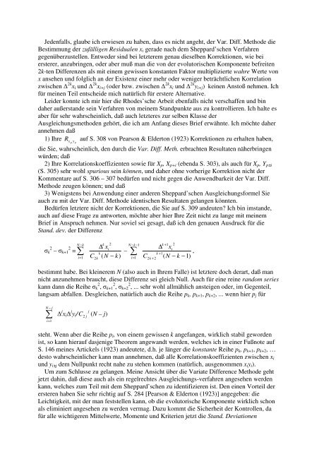
Jedenfalls, glaube ich erwiesen zu haben, dass es nicht angeht, der Var. Diff. Methode dieBestimmung der zufälligen Residualen x i gerade nach dem Sheppard’schen Verfahrengegenüberzustellen. Entweder sind bei letzterem genau dieselben Korrektionen, wie beiersterer, anzubringen, oder aber muß man die von der evolutorischen Komponente befreiten2k-ten Differenzen als mit einem gewissen konstanten Faktor multiplizierte wahre Werte vonx ansehen und folglich an der Existenz einer mehr oder weniger beträchtlichen Korrelationzwischen ! 2k x i und ! 2k x i+j (oder bzw. zwischen ! 2k x i und ! 2k y i+j ) keinen Anstoß nehmen. Ichfür meinen Teil entscheide mich natürlich für erstere Alternative.Leider konnte ich mir hier die Rhodes’sche Arbeit ebenfalls nicht verschaffen und bindaher außerstande sein Verfahren von meinem Standpunkte aus zu kontrollieren. Ich halte esaber für sehr wahrscheinlich, daß auch letzteres zur selben Klasse derAusgleichungsmethoden gehört, die ich am Anfang dieses Brief erwähnte. Ich möchte daherannehmen daß1) Ihre R auf S. 308 von Pearson & Elderton (1923) Korrektionen zu erhalten haben,x p y pdie Sie, wahrscheinlich, den durch die Var. Diff. Meth. erbrachten Resultaten näherbringenwürden; daß2) Ihre Korrelationskoeffizienten sowie für X p , X p+i (ebenda S. 303), als auch für X p , Y p±i(S. 305) sehr wohl spurious sein können, und daher ohne vorherige Korrektion nicht derKommentare auf S. 306 – 307 bedürfen und nicht gegen die Anwendbarkeit der Var. Diff.Methode zeugen können; und daß3) Wenigstens bei Anwendung einer anderen Sheppard’schen Ausgleichungsformel Sieauch zu mit der Var. Diff. Methode identischen Resultaten gelangen könnten.Bedürfen letztere nicht der Korrektionen, die Sie auf S. 309 andeuten? Ich bin imstande,auch auf diese Frage zu antworten, möchte aber hier Ihre Zeit nicht zu lange mit meinemBrief in Anspruch nehmen. Nur soviel sei gesagt, daß ich den genauen Ausdruck für dieStand. dev. der Differenz k 2 – k+1 2 = −=N k k 2∆ xiki 1 C2k( N − k)− 1k + 1 2∆ xik + 1i = 1 C2k+ 2( N − k −1)N k– −,bestimmt habe. Bei kleinerem N (also auch in Ihrem Falle) ist letztere doch derart, daß mannicht anzunehmen braucht, diese Differenz sei gleich Null. Auch für eine reine random serieskann dann die Reihe k 2 , k+1 2 , k+2 2 , ... sehr wohl allmählich ansteigen oder, im Gegenteil,langsam abfallen. Desgleichen, natürlich auch die Reihe p k , p k+1 , p k+2 , ... wenn hier p j fürN − ji=1jj! j x i ! j y i / C 2(N – j)steht. Wenn aber die Reihe p i , von einem gewissen k angefangen, wirklich stabil gewordenist, so kann hierauf dasjenige Theorem angewandt werden, welches ich in einer Fußnote aufS. 146 meines Artickels (1923) andeutete, d.h. je länger die konstante Reihe p k , p k+1 , p k+2 , …desto wahrscheinlicher kann man annehmen, daß alle Korrelationskoeffizienten zwischen x iund y i±j dem Nullpunkt recht nahe zu stehen kommen (natürlich, ausgenommen x i y i ).Um zum Schlusse zu gelangen. Meine Ansicht über die Variate Difference Methode gehtjetzt dahin, daß diese auch als ein regelrechtes Ausgleichungs-verfahren angesehen werdenkann, welches zum Teil mit dem Sheppard’schen zu identifizieren ist. Den einen Vorteil derersteren haben Sie sehr richtig auf S. 284 [Pearson & Elderton (1923)] angegeben: dieLeichtigkeit, mit der man feststellen kann, ob die evolutorische Komponente wirklich schonals eliminiert angesehen zu werden vermag. Dazu kommt die Sicherheit der Kontrollen, dafür alle wichtigeren Mittelwerte, Momente und Kriterien jetzt die Stand. Deviationen