kniga 7 - Probability and Statistics 1 - Sheynin, Oscar

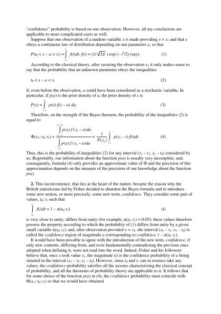
“confidence” probability is based on one observation. However, all my conclusions areapplicable to more complicated cases as well.Suppose that one observation of a random variable x is made providing x = x 1 and that xobeys a continuous law of distribution depending on one parameter a, so thatP(t 0 < x – a < t 1 ) = 1 t0tf(t)dt, f(t) = (1/2 π ) exp (– t 2 /2) (say). (1)According to the classical theory, after securing the observation x 1 it only makes sense tosay that the probability that an unknown parameter obeys the inequalitiest 0 < x – a < t 1 (2)if, even before the observation, a could have been considered as a stochastic variable. Inparticular, if p(a) is the prior density of a, the prior density of x is∞P(x) = p(a) f(x – a) da. (3)−∞Therefore, on the strength of the Bayes theorem, the probability of the inequalities (2) isequal to(x 1 ; t 0 ; t 1 ) =x −t1x −t∞−∞0p(a)f ( x − a)da1 1=p(a)f ( x − a)da111P(x 1) 1 t0tp(x 1 – t) f(t)dt. (4)Thus, this is the probability of inequalities (2) for any interval (x 1 – t 1 ; x 1 – t 0 ) considered byus. Regrettably, our information about the function p(a) is usually very incomplete, and,consequently, formula (4) only provides an approximate value of and the precision of thisapproximation depends on the measure of the precision of our knowledge about the functionp(a).2. This inconvenience, that lies at the heart of the matter, became the reason why theBritish statisticians led by Fisher decided to abandon the Bayes formula and to introducesome new notion, or more precisely, some new term, confidence. They consider some pair ofvalues, t 0 ; t 1 such thatt 1 t0f(t)dt = 1 – (t 0 ; t 1 )is very close to unity: differs from unity (for example, (t 0 ; t 1 ) = 0.05); these values thereforepossess the property according to which the probability of (1) differs from unity by a givensmall variable (t 0 ; t 1 ); and, after observation provided x = x 1 , the interval (x 1 – t 1 ; x 1 – t 0 ) iscalled the confidence region of magnitude a corresponding to confidence 1 – (t 0 ; t 1 ).It would have been possible to agree with the introduction of the new term, confidence, ifonly new contents, differing from, and even fundamentally contradicting the previous onesadopted when defining it, were not read into the word. Indeed, Fisher and his followersbelieve that, once x took value x 1 , the magnitude (i) is the confidence probability of a beingsituated in the interval (x 1 – t 1 ; x 1 – t 0 ). However, since t 0 and t 1 can in essence take anyvalues, the confidence probability satisfies all the axioms characterizing the classical conceptof probability, and all the theorems of probability theory are applicable to it. It follows thatfor some choice of the function p(a) in (4), the confidence probability must coincide with(x 1 ; t 0 ; t 1 ) so that we would have obtained(i)