Estimation Of Generalized Mixtures And Its Application ... - IEEE Xplore

More documents

Recommendations

Info

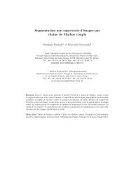
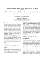
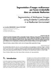
DELIGNON et al.: ESTIMATION OF GENERALIZED MIXTURES 1369B. Global Approach1) Markovian Model and Global Segmentation: In theglobal approach, each is estimated fromThe fieldis a Markov random field and we willconsider Ising’s model, which is the simplest one. In order tosimplify notations we will limit our presentation to the case oftwo classes; however, the generalization to any other numberof classes poses no particular problem.The distribution of is given bywithand(34)Fig. 3.Image 1: SEASAT image of the Brittany coast.if,if(35)IV. UNSUPERVISED IMAGE SEGMENTATIONIn this section, we propose some applications of differentgeneralized mixture estimators to the problem of unsupervisedimage segmentation. We shall consider two well known approaches:the “blind” approach and the “global” one. In theblind approach the generalized SEM, EM, and ICE algorithmsabove can be applied directly. In the global one we proposetwo adaptations of Gibbsian EM and ICE. For each methodwe specify here the reestimation formulas; the initialization ofdifferent algorithms is described in Section V.A. Blind ApproachThe “blind” approach consists of estimating the realizationof each from This is the simplest one and, generally,the least efficient. However, its “adaptive” version can be verycompetitive in some situations [26]. Let be priors andbe densities of the distribution of conditional toThe blind Bayesian strategy isifif(33)This strategy is made unsupervised by the direct use of theGSEM algorithm described above: One chooses a sequence ofpixels and considers that is the value of thegrey level at pixel In an “adaptive” version of the “blind”approach, one considers that priors depend on the positionof the pixel in The blind adaptive Bayesian strategy isthe same as above with instead of TheGSEM algorithm is modified as follows. Letbe the sequence obtained by sampling at a given iteration.In GSEM the priors are reestimated by the frequenciescomputed using all the sample points; in “adaptive” GSEM oneconsiders, for each a window centred at andare reestimated by frequencies computed from Letus note that in “adaptive” GSEM the sequence of pixelshas to cover In the following, the generalizedadaptive SEM, EM, and ICE will be denoted by GASEM,GAEM, and GAICE.Thus, is defined by The random variableswill be assumed independent conditionally to and furthermore,the distribution of each conditional to will beassumed equal to its distribution conditional on Underthese hypothesis all distributions of conditional to are definedby the two distributions of conditional torespectively. Let us denote by the densities of thesedistributions and assume that they belong to Pearson’s system.They are thus given by parametersand, respectively.Finally, all distributions of conditional to are definedby and thus defines the distributionofThe possibility of simulating realizations of according toits posterior, i.e. conditional to distribution constitutes themain interest of this model.2) Generalized Global ICE (GGICE): According to theICE principle, let us suppose that is observable. We havethen to proposeThere exist numerous estimators of the parameterfrom such as the coding method [2], the least squareserror method [12], or the maximum likelihood estimate [35].As our model is very simple, we can use an empiricalfrequency based estimator. In fact, there exists a simple linkbetween and probabilities “ knowing that theneighborhood of contains times,” where can take 0,1, 2, 3, 4 as values. For instance, if we take we select inthe image a sample of neighborhoods of containingtwo and two The probability “ knowing thatthe neighborhood of contains two ” is estimated by theproportion of the sample giving On the other handthis probability is given by(36)which gives an estimated value ofWe take for the same estimator as in the case ofindependent mixture, Section III-A.
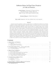
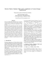
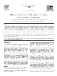
1370 IEEE TRANSACTIONS ON IMAGE PROCESSING, VOL. 6, NO. 10, OCTOBER 1997Fig. 4. Unsupervised segmentation results of Image 1, Fig. 3.Fig. 5.Image 2 and its unsupervised segmentations.Finally, the GGICE runs as follows.1) Sample according to .2) Compute .3) Consider andand apply 2–5 of the end of SectionIII-A.3) Generalized Gibbsian EM (GGEM)The difference between GGICE above and GGEM is situatedat the noise parameter reestimation level. We havetwo noise distributions conditional to the two classes and weare interested in estimating the four first moments of eachof them. In the case of GGICE, these two problems aretreated separately by considering the partition onandof the set ofpixels In the case of GGEM each of them is treated by theuse of the whole set Let us put(37)The first four moments of the noise corresponding to the firstclassare given byV. EXPERIMENTSWe present in this section some results of numerical applications.Let us note that in the global case the segmentation isperformed by the maximizer of posterior marginals (MPM)and, in the local case, it is performed by the rule (33).Thus, unsupervised segmentation algorithms considered in thispaper mainly differ by their parameter estimation step: Wewill note them by the parameter estimation method used. Forinstance, GEM will denote the local segmentation (33) basedon parameters estimated with generalized EM, GGEM willdenote the global MPM segmentation based on parametersestimated with generalized Gibbsian EM, and so on. The firstsection is devoted to synthetic images and in the second onewe deal with three real radar images.The initialization of GEM, GSEM, and GICE is as follows.We assume that we have a mixture of two Gaussian distributions.With denoting the cumulated histogram we takeandIn order to initialize GGEM and GGICE, we use thesegmentation obtained by the blind unsupervised method,which gives The noise parameters are initialized by thefinal parameters obtained in the parameter estimation step ofthe blind unsupervised method used.andforUse analogous formulas for the second class.(38)(39)A. Experiments on a Synthetic ImageLet us consider a binary image “ring” given in Fig. 2. Whiteis class 1 and black class 2. The class 1 is corrupted by a betanoise of the first kind (family in Pearson’s system) and theclass 2 is noised by a beta noise of the second kind (familyin Pearson’s system). The parameters defining the noisedistributions, their estimates with different methods, and thesegmentation error rates are given in Table I. The noisy versionof the ring image and some segmentation results are presentedin Fig. 2. We have taken the same means and variances on
Page 1 and 2: 1364 IEEE TRANSACTIONS ON IMAGE PRO
Page 5: 1368 IEEE TRANSACTIONS ON IMAGE PRO

Estimation Of Generalized Mixtures And Its Application ... - IEEE Xplore

You also want an ePaper? Increase the reach of your titles

Delete template?

Save as template?