Removing the Stiffness from Interfacial Flows with Surface Tension

More documents

Recommendations

Info

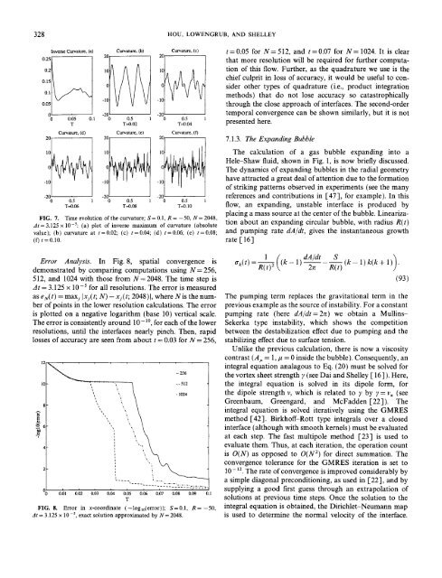
FLOWS WITH SURFACE TENSION 327face tension and the unstable stratification causes the interfaceto rapidly develop a ramified spatial structure.A time sequence of inteface positions is shown in Fig. 4using N=2048 and At= 3.125 × 10 -5. The second-orderlinear propagator method is used, and the time step ischosen small enough so as to effectively eliminate time-steppingerrors from the computation. At early times, threerising and falling fingers of fluid form. As time progresses,the tips of these fingers thicken and begin to resemblebubbles. The necks of the fastest moving fingers begin tonarrow and their sides approach tangentially. The othernecks appear to follow suit. These necks become localizedjets, fluxing fluid from the bulk into the bubbles. At latertimes, the sides of the necks seem to self-intersect or pinch.However, a close-up of the neck region (box (f)) of thetopmost bubble reveals that the pinching has not yet takenplace by t = 0.10 and that the neck still has a nonzero width.As the necks narrow, however, it becomes more and moredifficult to maintain resolution. This is because the alternatepoint discretization of the Birkhoff-Rott integral requires aminimum width of six or seven grid lengths in the neckregion for accuracy [ 8 ]. This effect is illustrated in Fig. 5,where the interface positions are compared at t = 0.10 withN= 1024 and N---2048. Although pinching has alreadytaken place in the N = 1024 calculation, it is unphysical. Therrrinimum width of the neck as a function of time is shownin Fig. 6 for several spatial resolutions: N= 512, N= 1024and N=2048 (again using the same time step Lit=3.125 x 10-5). The width is computed by minimizing thedistance function between the bounding curves, which arerepresented by Fourier polynomials. The width of the neckdecreases rapidly at early times. By t = 0.065 with N= 512,the neck is but one grid length wide, and the calculationbecomes inaccurate. The higher resolution calculations21.510.50-0.5-1-1.5-2 1024i0LiI 2FIG. 5. Comparison of Hele-Shaw interfaces at t = 0.10 for differentspatial resolutions: the left corresponds to N= 1024 and the right toN=2048; S=0.1, R= -50, At= 3.125 x l0 -5.)L32O480.12-- 512-.- 10240.1 - 20480.08~ 0.0~0.0,t0.020 5 6 7 8 :, 10T x 10 .2FIG. 6. Minimum distance to pinching for N= 512, N= 1024, andN= 2048; S = 0.1, R = -50, At = 3.125 x 10 -5.indicate that the narrowing slows shortly thereafter.However, by t = 0.08, the N = 1024 calculation has a neckwidth of only five grid lengths, and that calculation becomesinaccurate. But by using N = 2048, the width is seen tosaturate after t= 0.08 and shows only a slight furtherdecrease by t = 0.10. The neck region is 11 of its grid lengthswide. Presumably, the width of the neck region scales withthe surface tension, although this has not been studied indetail.This lack of self-intersection in the neck region is consistentwith behavior found by Goldstein, Pesci, and Shelley[ 18 ] in asymptotic models of jets in Hele-Shaw flows. Theirmodelling suggests also that the minimum neck widthdecreases by a factor of two with a fourfold decrease in thesurface tension. It is only in the limit of zero surface tensionthat their model equation predicts the breaking of the neck.They do consider other cases, however, where the surfacetension does not prevent the pinching of material interfaces.Figure 7 shows the evolution of the curvature. The topleft plot shows the inverse of the maximum absolute curvature.Vanishing in this plot would correspond to adivergence of the curvature. At early times, there is a rapidincrease in the curvature (a decrease in the plot). It peaksaround t= 0.015 and then begins to decrease. This lastsuntil t -- 0.05. The curvature then refocuses and the processrepeats itself several times. By the end of the computation,the curvature has nearly reached again its peak at t = 0.015.The other plots in Fig. 7 show x as a function of ~ at severaltimes; these graphs indicate that in fact, the curvaturesaturates at one part of the interface and refocuses inanother, leading to a very complicated overall structure.The boundaries of the narrow neck regions are indicated bya pairs of closely spaced peaks of like signed curvature. Thephenomenon of saturation and refocussing will be seenagain in the context of inertial vortex sheets.
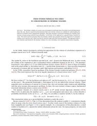
328 HOU, LOWENGRUB, AND SHELLEY0.250.20.150A0.05Inverse Curvature, (a)20110101Curvature, (b)0 0.05 O. 1 0.5TT=0.02Curvature, (d)20 20110-10101O~ilCurvature, (e)Curvature, (c)-200 0.5 0.5-200.5T--0.06 T--0.08 T--0.10200-10-20 0 0.5T---0.04200-10Curvature, (f)FIG. 7. Time evolution of the curvature; S = 0.1, R = -50, N = 2048,At= 3.125 x 10-5: (a) plot of inverse maximum of curvature (absolutevalue); (b) curvature at t=0.02; (c) t=0.04; (d) t=0.06; (e) t=0.08;(f) t = 0.10.Error Analysis. In Fig. 8, spatial convergence isdemonstrated by comparing computations using N= 256,512, and 1024 with those from N= 2048. The time step isAt = 3.125 × 10-5 for all resolutions. The error is measuredas eN(t) = maxj Ixj(t; N) - xj(t; 2048)1, where Nis the numberof points in the lower resolution calculations. The erroris plotted on a negative logarithm (base 10) vertical scale.The error is consistently around 10- lO, for each of the lowerresolutions, until the interfaces nearly pinch. Then, rapidlosses of accuracy are seen from about t = 0.03 for N = 256,~ 6"712 ~ ~ . _ _113842Ci0.01 0.02 0.(13-- 256-~ -.- 512i~ - 1024' ~ .,\~,, ,.\,i .ii i i i i . . . . . i'- ....0.04 0.05 0.06 0.07 0.08 0.09 0.1TFIG. 8. Error in x-coordinate (-loglo(error)); S=0.1, R=-50,Jt = 3.125 x 10-5, exact solution approximated by N= 2048.t=0.05 for N=512, and t=0.07 for N= 1024. It is clearthat more resolution will be required for further computationof this flow. Further, as the quadrature we use is thechief culprit in loss of accuracy, it would be useful to considerother types of quadrature (i.e., product integrationmethods) that do not lose accuracy so catastrophicallythrough the close approach of interfaces. The second-ordertemporal convergence can be shown similarly, but it is notpresented here.7.1.3. The Expanding BubbleThe calculation of a gas bubble expanding into aHele-Shaw fluid, shown in Fig. 1, is now briefly discussed.The dynamics of expanding bubbles in the radial geometryhave attracted a great deal of attention due to the formationof striking patterns observed in experiments (see the manyreferences and contributions in [47 ], for example). In thisflow, an expanding, unstable interface is produced byplacing a mass source at the center of the bubble. Linearizationabout an expanding circular bubble, with radius R(t)and pumping rate dA/dt, gives the instantaneous growthrate [ 16 ]1(dA/dtak(t) =R--~ (k- 1) --2reS\-- (k- 1)k(k+ 1)).R(t)(93)The pumping term replaces the gravitational term in theprevious example as the source of instability. For a constantpumping rate (here dA/dt=2g) we obtain a Mullins-Sekerka type instability, which shows the competitionbetween the destabilization effect due to pumping and thestabilizing effect due to surface tension.Unlike the previous calculation, there is now a viscositycontrast (A, = 1,/t = 0 inside the bubble). Consequently, anintegral equation analagous to Eq. (20) must be solved forthe vortex sheet strength y (see Dai and Shelley [ 16 ] ). Here,the integral equation is solved in its dipole form, forthe dipole strength v, which is related to y by ? = v~ (seeGreenbaum, Greengard, and McFadden [22]). Theintegral equation is solved iteratively using the GMRESmethod [42]. Birkhoff-Rott type integrals over a closedinterface (although with smooth kernels) must be evaluatedat each step. The fast multipole method [23] is used toevaluate them. Thus, at each iteration, the operation countis O(N) as opposed to O(N 2) for direct summation. Theconvergence tolerance for the GMRES iteration is set to10-x2. The rate of convergence is improved considerably bya simple diagonal preconditioning, as used in [22], and bysupplying a good first guess through an extrapolation ofsolutions at previous time steps. Once the solution to theintegral equation is obtained, the Dirichlet-Neumann mapis used to determine the normal velocity of the interface.
Page 4 and 5: FLOWS WITH SURFACE TENSION 315lower
Page 6 and 7: FLOWS WITH SURFACE TENSION 317Again
Page 8 and 9: FLOWS WITH SURFACE TENSION 319integ
Page 10 and 11: FLOWS WITH SURFACE TENSION 321The s
Page 12 and 13: FLOWS WITH SURFACE TENSION 323updat
Page 14 and 15: FLOWS WITH SURFACE TENSION 325arcle
Page 18 and 19: FLOWS WITH SURFACE TENSION 329This
Page 20 and 21: FLOWS WITH SURFACE TENSION 331facto
Page 22 and 23: FLOWS WITH SURFACE TENSION 333of th
Page 24 and 25: FLOWS WITH SURFACE TENSION 335singu
Page 26 and 27: FLOWS WITH SURFACE TENSION 337(2) C

Removing the Stiffness from Interfacial Flows with Surface Tension

You also want an ePaper? Increase the reach of your titles

Delete template?

Save as template?