Removing the Stiffness from Interfacial Flows with Surface Tension

More documents

Recommendations

Info

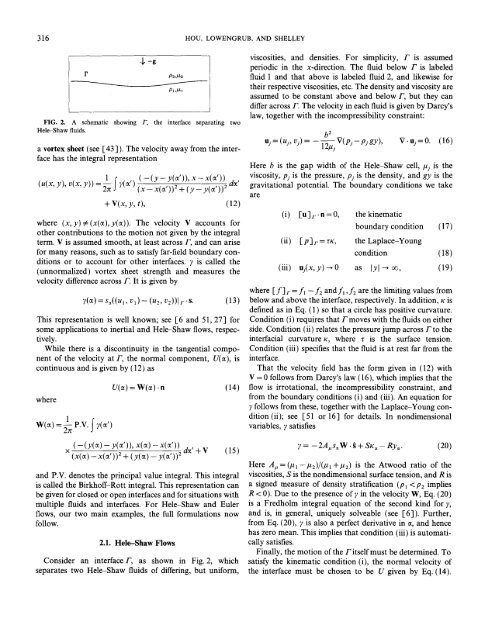
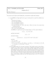
FLOWS WITH SURFACE TENSION 315lower order terms in the evolution. There is also an equationanalogous to Eq. (8) for L. Such a reformulation of fluidinterface evolution, as in Eq. (11 ), is a "small scale decomposition."It is within the small scale decomposition thatimplicit integration or linear propagator methods can beapplied to a high order linear term. With periodic boundaryconditions, these methods are explicit in Fourier space andhave no high-order time step constraint. The time-steppingmethods are coupled to spectrally accurate spatial discretizations.Small scale decompositions are given also formore general Hele-Shaw flows and for interface flows underthe Euler equations.An example of what is possible with these methods is seenin Fig. 1, which shows the simulation of a gas bubbleexpanding into a Hele-Shaw fluid (see [ 15, 16]) over longtimes. From the competition of surface tension with the fluidpumping, this simulation shows the development oframification through successive tip-splitting events and thecompetition between adjacent fingers. This simulation isalso spectrally accurate in space and uses a second-order intime linear propagator method for integrating the smallscaledecomposition. There are no high-order time stepconstraints. The fluid velocity is calculated using the fastmultipole method [23], and GMRES [42] is used to solvethe integral equation that arises from having a viscosity con-" trast [22]. The operation count is O(N) at each time-step,where N is the number of points describing the boundary.Here N= 4096, S = 0.001, and At = 0.001. The time step is103 times larger than that used by Dai and Shelley [ 16] incomputations of a similar flow using an explicit method15with a lesser number of points, and the interface here hasdeveloped far more structure.The organization of the paper is as follows. In Section 2,boundary integral formulations are given for the motion offluid interfaces under surface tension in both Hele-Shawand two-dimensional Euler flows. The interface is interpretedas a vortex sheet whose normal velocity is determinedby the Birkhoff-Rott integral. Its vortex sheetstrength is determined by the equations of motion andboundary conditions. In Section 3, the source of stiffness inthese problems is discussed and motivated by thegeneralized linear stability analysis of Beale, Hou, andLowengrub [10-12]. In Section4, the Birkhoff-Rottintegral is carefully examined. It is shown that this integral,asymptotically at small scales, becomes a Hilbert transformof the sheet strength over a flat interface, with a variableprefactor. In Section 5, the description of the interface isreformulated in terms of 0 and L. This step makes thevariable coefficient depend only upon time, and at smallscales, the leading order terms are only nonlocal through aHilbert transform. This leads to small scale decompositionsfor the evolution problems. In Section 6, numerical methodsare discussed. This includes second-order integrationmethods that exploit the small scale decomposition toremove the high-order stiffness, generalizations to higherorder time discretizations, as well as other related numericalissues such as spectrally accurate spatial discretizations. InSection 7 the results of numerical simulations using thesemethods are presented. These results include the motionof Hele-Shaw interfaces moving under the competinginfluences of gravity and surface tension, in addition to theexpanding gas bubble. The roll-up and collision of vortexsheets with surface tension in an Euler flow is also given.Concluding remarks are given in Section 8.10-5-10-15-1I I I I I-10 -5 0 5 10 15Time =0 to 45FIG. 1.An expanding Hele-Shaw bubble.2. THE FORMULATIONIn this section, boundary integral formulations are givenfor two illustrative incompressible flows. The first describesthe motion of an interface separating two Hele-Shaw fluidsof differing densities and viscosities. The second describesthe motion of a vortex sheet in a two-dimensional, inviscidfluid. As the concept of a vortex sheet arises also in theHele-Shaw case, this second case is referred to as an inertialvortex sheet.Consider an incompressible and irrotational velocity fieldin two dimensions given in terms of a velocity potential:(u,v)=V~. Suppose that ~b has a jump across aparametrized interface F= (x(~), y(0~)), but that its normalderivative is continuous (see Fig. 2). This implies that thevelocity has a tangential discontinuity across F while thecomponent normal to F is continuous (i.e., the kinematicboundary condition is satisfied). Such an interface is called
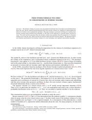
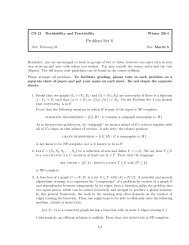
316 HOU, LOWENGRUB, AND SHELLEYP$-~pa,/z2FIG. 2. A schematic showing F, the interface separating twoHele-Shaw fluids.a vortex sheet (see [43 ] ). The velocity away from the interfacehas the integral representation(u(x, y), v(x, Y))1 f (--(y-y(og)),x-x(og)) , ,J ~(~') (x - x(¢)) ~ + (y- y(¢))= ao~+ V(x, y, t), (12)where (x,y)¢(x(oQ, y(ct)). The velocity V accounts forother contributions to the motion not given by the integralterm. V is assumed smooth, at least across F, and can arisefor many reasons, such as to satisfy far-field boundary conditionsor to account for other interfaces. 7 is called the(unnormalized) vortex sheet strength and measures thevelocity difference across F. It is given by~(~)=s,((u,, v~)-(u2, v2))l~.s.This representation is well known; see [6 and 51, 27] forsome applications to inertial and Hele-Shaw flows, respectively.While there is a discontinuity in the tangential componentof the velocity at F, the normal component, U(00, iscontinuous and is given by (12) aswhere1w(~) =~ P.V. f ~(~')U(~)=W(~).nviscosities, and densities. For simplicity, F is assumedperiodic in the x-direction. The fluid below F is labeledfluid 1 and that above is labeled fluid 2, and likewise fortheir respective viscosities, etc. The density and viscosity areassumed to be constant above and below F, but they candiffer across F. The velocity in each fluid is given by Darcy'slaw, together with the incompressibility constraint:b 2oj= (uj, vj) = 12ktjV(ps-psgy), V.uj= O. (16)Here b is the gap width of the Hele-Shaw cell, pj is theviscosity, pj is the pressure, Ps is the density, and gy is thegravitational potential. The boundary conditions we takeare(i) [U]r'n =0, the kinematicboundary condition (17)(ii) [ P ] r = zK, the Laplace-Youngcondition (18)(iii) uj(x,y)-~O as lyl---' ~, (19)where [ f ] r = fl - f2 and fl, f2 are the limiting values from(13) below and above the interface, respectively. In addition, x isdefined as in Eq. (1) so that a circle has positive curvature.Condition (i) requires that F moves with the fluids on eitherside. Condition (ii) relates the pressure jump across F to theinterfacial curvature x, where z is the surface tension.Condition (iii) specifies that the fluid is at rest far from theinterface.That the velocity field has the form given in (12) withV = 0 follows from Darcy's law (16), which implies that the(14) flow is irrotational, the incompressibility constraint, andfrom the boundary conditions (i) and (iii). An equation for7 follows from these, together with the Laplace-Young condition(ii); see [51 or 16] for details. In nondimensionalvariables, 7 satisfies(- (y(0Q- y(0()), x(0Q - x(ct'))x (x(~) -x(~')) 2 + (y(~) - y(~,)12d~'+V (15)and P.V. denotes the principal value integral. This integralis called the Birkhoff-Rott integral. This representation canbe given for closed or open interfaces and for situations withmultiple fluids and interfaces. For Hele-Shaw and Eulerflows, our two main examples, the full formulations nowfollow.2.1. Hele-Shaw FlowsConsider an interface F, as shown in Fig. 2, whichseparates two Hele-Shaw fluids of differing, but uniform,7 = -2Aus~W. ~ + Sx~- Rye. (20)is the Atwood ratio of theviscosities, S is the nondimensional surface tension, and R isa signed measure of density stratification (Pl
Page 6 and 7: FLOWS WITH SURFACE TENSION 317Again
Page 8 and 9: FLOWS WITH SURFACE TENSION 319integ
Page 10 and 11: FLOWS WITH SURFACE TENSION 321The s
Page 12 and 13: FLOWS WITH SURFACE TENSION 323updat
Page 14 and 15: FLOWS WITH SURFACE TENSION 325arcle
Page 16 and 17: FLOWS WITH SURFACE TENSION 327face
Page 18 and 19: FLOWS WITH SURFACE TENSION 329This
Page 20 and 21: FLOWS WITH SURFACE TENSION 331facto
Page 22 and 23: FLOWS WITH SURFACE TENSION 333of th
Page 24 and 25: FLOWS WITH SURFACE TENSION 335singu
Page 26 and 27: FLOWS WITH SURFACE TENSION 337(2) C

Removing the Stiffness from Interfacial Flows with Surface Tension

Create successful ePaper yourself

Delete template?

Save as template?