Removing the Stiffness from Interfacial Flows with Surface Tension

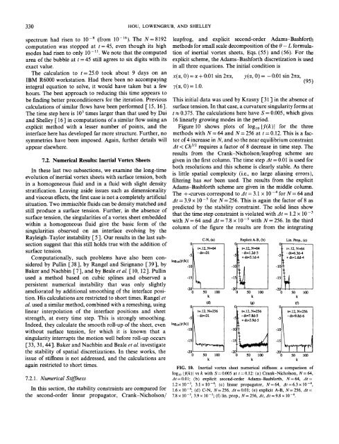
330 HOU, LOWENGRUB, AND SHELLEYspectrum had risen to 10 -8 (from 10-16). The N= 8192computation was stopped at t = 45, even though its highmodes had risen to only 10-11. We note that the computedarea of the bubble at t = 45 still agrees to six digits with itsexact value.The calculation to t = 25.0 took about 9 days on anIBM R6000 workstation. Had there been no accompayingintegral equation to solve, it would have taken but a fewhours. The best approach to reducing this time appears tobe finding better preconditioners for the iteration. Previouscalculations of similar flows have been performed [ 15, 16].The time step here is 103 times larger than that used by Daiand Shelley [ 16 ] in computations of a similar flow using anexplicit method with a lesser number of points, and theinterface here has developed far more structure. Further, nosymmetries have been imposed. Again, further details willappear elsewhere.7.2. Numerical Results: Inertial Vortex SheetsIn these last two subsections, we examine the long-timeevolution of inertial vortex sheets with surface tension, bothin a homogeneous fluid and in a fluid with slight densitystratification. Leaving aside issues such as dimensionalityand viscous effects, the first case is not a completely artificialsituation. Two immiscible fluids can be density matched andstill produce a surface tension. Further, in the absence ofsurface tension, the singularities of a vortex sheet embeddedwithin a homogeneous fluid give the basic form of thesingularities observed on an interface evolving by theRayleigh-Taylor instability [ 5 ]. Our results in the last subsectionsuggest that this still holds true with the addition ofsurface tension.Computationally, such problems have also been consideredby Pullin [ 38 ], by Rangel and Sirignano [ 39], byBaker and Nachbin [7], and by Beale et al. [ 10, 12]. Pullinused a method based on cubic splines and observed apersistent numerical instability that was only slightlyameliorated by additional smoothing of the interface position.His calculations are restricted to short times. Rangel etaL used a similar method, combined with a remeshing, usinglinear interpolation of the interface positions and sheetstrength, at every time step. This is strongly smoothing.Indeed, they calculate the smooth roll-up of the sheet, evenwithout surface tension, for which it is known that asingularity interrupts the motion well before roll-up occurs[33, 31, 44]. Baker and Nachbin and Beale et al. investigatethe stability of spatial discretizations. In these works, theissue of stiffness is not addressed, and the calculations areagain restricted to short times.7.2.1. Numerical StiffnessIn this section, the stability constraints are compared forthe second-order linear propagator, Crank-Nicholson/leapfrog, and explicit second-order Adams-Bashforthmethods for small scale decomposition of the 0 - L formulationof inertial vortex sheets, Eqs. (55) and (56). For theexplicit scheme, the Adams-Bashforth discretization is usedin all three equations. The initial condition isx(~, 0) = ~ + 0.01 sin 2zt~, y(ct, 0) -- -0.01 sin 2~,7(~, 0)= 1.0.(95)This initial data was used by Krasny [31] in the absence ofsurface tension. In that case, a curvature singularity forms att ~ 0.375. The calculations here have S = 0.005, which gives16 linearly growing modes in the period.Figure 10 shows plots of log10 IP(k)F for the threemethods with N = 64 and N= 256 at t = 0.12. This is a factorof 4 increase in N, and so the near equilibrium constraintAt < Ch 3/2 requires a factor of 8 decrease in time step. Theresults from the Crank-Nicholson/leapfrog scheme aregiven in the first column. The time step At = 0.01 is used forboth resolutions and this scheme is clearly stable. As thereis little spatial complexity (i.e., no large aliasing errors),filtering has not been used. The results from the explicitAdams-Bashforth scheme are given in the middle column.The +-curves correspond to At = 3.1 x 10-4 for N = 64 andAt = 3.9 x 10-5 for N= 256. This is again the factor of 8 aspredicted by the stability constraint. The solid lines showthat the time step constraint is violated with At = 1.2 x 10 -3with N= 64 and At = 7.8 x 10-5 with N = 256. In the thirdcolumn of the figure the results are from the integratingl°glol$'(k)!l 0C-N, (a)° i , t=.12, N=64I-15 ~I]- dt=.01o-5-IO-15Expficit A-B. (b)t=. 12, N=64- dt=l.2d-3+ dt~3.1d-4Lin. Prop., (c)-2c-20 I50 1000 50 100kkk-2C-2-2050 100 50 I00 0 50 100k k k(d)(t=.12, N=256(g)t=.12, N=256(Dt=.12, N=256-5 - dt=.01- dt=7.Sd-5- dt=9.Sd-6-5+ dt=3.9d-5logaol~'(k)l-K-15-10:-10-15-10-15t=.12, N=64- dt=6.3d-4+ dt=l.6d-4FIG. 10. Inertial vortex sheet numerical stiffness: a comparison oflog10 I~(k)l vs k with S= 0.005 at t = 0.12: (a) Crank-Nicholson, N= 64,At = 0.01; (b) explicit second-order Adams-Bashforth, N= 64, At =1.2 × 10-3, 3.1 x 10-4; (c) linear propagator, N= 64, At = 6.3 x 10-4,1.6x 10-4; (d) C-N, N=256, At=0.01; (e) explicit A-B, N=256, At=7.8 x 10-5, 3.9 × 10 -5; (f) lin. prop., N= 256, At, At = 9.8 x 10-6.