Spatial filter masks Order-Statistic

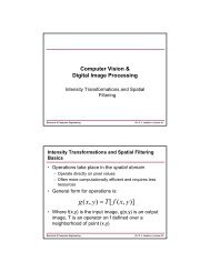
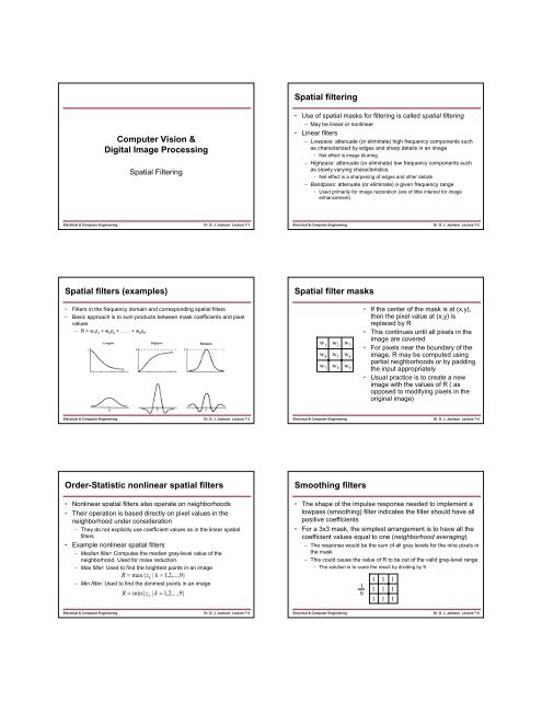
Spatial filteringComputer Vision &Digital Image ProcessingSpatial Filtering• Use of spatial masks for filtering is called spatial filtering– May be linear or nonlinear• Linear filters– Lowpass: attenuate (or eliminate) high frequency components suchas characterized by edges and sharp details in an image• Net effect is image blurring– Highpass: attenuate (or eliminate) low frequency components suchas slowly varying characteristics• Net effect is a sharpening of edges and other details– Bandpass: attenuate (or eliminate) a given frequency range• Used primarily for image restoration (are of little interest for imageenhancement)Electrical & Computer EngineeringDr. D. J. Jackson Lecture 7-1Electrical & Computer EngineeringDr. D. J. Jackson Lecture 7-2Spatial filters (examples)Spatial filter masks• Filters in the frequency domain and corresponding spatial filters• Basic approach is to sum products between mask coefficients and pixelvaluesw 9 w 7 w 8partial neighborhoods or by paddingthe input appropriately• If the center of the mask is at (x,y),then the pixel value at (x,y) isreplaced by R• This continues until all pixels in thew 1 w 2 w 3image are covered• For pixels near the boundary of thew 4 w 5 w 6 image, R may be computed using• Usual practice is to create a newimage with the values of R ( asopposed to modifying pixels in theoriginal image)– R = w 1 z 1 + w 2 z 2 + . . . . + w 9 z 9Dr. D. J. Jackson Lecture 7-4Electrical & Computer EngineeringDr. D. J. Jackson Lecture 7-3Electrical & Computer EngineeringOrder-Statistic nonlinear spatial filters• Nonlinear spatial filters also operate on neighborhoods• Their operation is based directly on pixel values in theneighborhood under consideration– They do not explicitly use coefficient values as in the linear spatialfilters• Example nonlinear spatial filters– Median filter: Computes the median gray-level value of theneighborhood. Used for noise reduction.– Max filter: Used to find the brightest points in an imageR = max{ zk| k = 1,2,...,9}– Min filter: Used to find the dimmest points in an imageR = min{ z | k = 1,2,...,9}kSmoothing filters• The shape of the impulse response needed to implement alowpass (smoothing) filter indicates the filter should have allpositive coefficients• For a 3x3 mask, the simplest arrangement is to have all thecoefficient values equal to one (neighborhood averaging)– The response would be the sum of all gray levels for the nine pixels inthe mask– This could cause the value of R to be out of the valid gray-level range• The solution is to scale the result by dividing by 9191 1 11 1 11 1 1Electrical & Computer EngineeringDr. D. J. Jackson Lecture 7-5Electrical & Computer EngineeringDr. D. J. Jackson Lecture 7-6

Averaging filter exampleSmoothing filter examplesElectrical & Computer EngineeringDr. D. J. Jackson Lecture 7-7Electrical & Computer EngineeringDr. D. J. Jackson Lecture 7-8Smoothing filters (continued)Median filtering example• One problem with the lowpassfilter is it blurs edges and othersharp details• If the intent is to achieve noisereduction, one approach can beto use median filtering– The value of each pixel isreplaced by the median pixelvalue in the neighborhood (asopposed to the average)– Particularly effective when thenoise consists of strong, spikelike components and edgesharpness is to be preserved• The median m of a set of valuesis such that half of the values aregreater than m and half are lessthan m• To implement, sort the pixelvalues in the neighborhood,choose the median and assignthis value to the pixel of interest• Forces pixels with distinctintensities to be more like theirneighborsElectrical & Computer EngineeringDr. D. J. Jackson Lecture 7-9Electrical & Computer EngineeringDr. D. J. Jackson Lecture 7-10Sharpening filtersSharpening filters (continued)• The shape of the impulse response needed to implement ahighpass (sharpening) filter indicates the filter should havepositive coefficients near its center and negative coefficientsin the outer periphery• For a 3x3 mask, the simplest arrangement is to have thecenter coefficient positive and all others negative19-1 -1 -1-1 8 -1-1 -1 -1• Note the sum of the coefficients is zero– When the mask is over a constant or slowly varying region the outputis zero or very small• This filter eliminates the zero-frequency term• Eliminating this term reduces the average gray-level value in the image tozero (will reduce the global contrast of the image)• Result will be a somewhat edge-enhanced image over a darkbackground• Reducing the average gray-level value to zero implies somenegative gray levels– The output should be scaled back into an appropriate range [0, L-1](or [1,256] for a 256 gray-level colormap MATLAB image)Electrical & Computer EngineeringDr. D. J. Jackson Lecture 7-11Electrical & Computer EngineeringDr. D. J. Jackson Lecture 7-12

Highpass filter exampleSharpening filters (continued)• A highpass filter may be computed as:Highpass = Original - Lowpass• Multiplying the original by an amplification factor yields ahighboost or high-frequency-emphasis filterHighboost = A(Original)− Lowpass= ( A −1)(Original)+ Original − Lowpass= ( A −1)(Original)+ Highpass– If A>1, part of the original image is added to the highpass result(partially restoring low frequency components)– Result looks more like the original image with a relative degree ofedge enhancement that depends on the value of A– May be implemented with the center coefficient value w=9A-1 (A≥1)Electrical & Computer EngineeringDr. D. J. Jackson Lecture 7-13Electrical & Computer EngineeringDr. D. J. Jackson Lecture 7-14Highboost filter exampleDerivative FunctionsA=1.15A=1.1A=1.2• A basic first-order derivative of a 1-D function, f(x),is the difference∂f= f ( x + 1) − f ( x)∂x• The second-order derivative of f(x) is the difference2∂ f= f ( x + 1) + f ( x −1)− 2 f ( x)2∂xElectrical & Computer EngineeringDr. D. J. Jackson Lecture 7-15Electrical & Computer EngineeringDr. D. J. Jackson Lecture 7-16Derivative FunctionsDerivative filters• Differentiation may be used for edge enhancement (detailsharpening)• The most common method for differentiating is the gradient.• For f(x,y) the gradient of f at (x,y) is defined as:• With a magnitude of:⎡∂f⎤⎢ ⎥∇f= ⎢∂ ∂ f x ⎥⎢ ⎥⎢⎣∂y⎥⎦22⎡⎛∂f⎞ ⎛ ∂f⎞ ⎤∇f= mag(∇f) = ⎢⎜⎟ + ⎜ ⎟ ⎥⎢⎣⎝ ∂x⎠ ⎝ ∂y⎠ ⎥⎦1/ 2Electrical & Computer EngineeringDr. D. J. Jackson Lecture 7-17Electrical & Computer EngineeringDr. D. J. Jackson Lecture 7-18

Derivative filters (continued)z 1 z 2 z 3z 4 z 5 z 6z 7 z 8 z 9• The magnitude of the gradient at z 5 can be approximated ina number of ways• The simplest is to use the difference (z 5 -z 8 ) in the x directionand (z 5 -z 6 ) in the y direction22 1/ 2∇f= [( z5 − z8)+ ( z5− z6)]• or approximated as∇f≈| z5 − z8| + | z5− z6|Derivative filters (continued)• A cross difference may also be used to approximate themagnitude of the gradient∇f= [( zz22 1/ 25− z9)+ ( z6−8)]∇f≈| z5 − z9| + | z6− z8|• This can be implemented by taking the absolute value of theresponse of the following two masks (the Roberts crossgradientoperators) and summing the results1 00 -10 1-1 0Electrical & Computer EngineeringDr. D. J. Jackson Lecture 7-19Electrical & Computer EngineeringDr. D. J. Jackson Lecture 7-20Derivative filters (continued)Derivative filters (continued)• Extension to a 3x3 mask yields the following∇f ≈| ( z7 + z8+ z9)− ( z1+ z2+ z3)| + | ( z3+ z6+ z9)− ( z1+ z4+ z7) |• The difference between the first and third rowsapproximates the derivative in the x direction• The difference between the first and third columnsapproximates the derivative in the y direction• The Prewitt operator masks may be used to implement theabove approximation-1 -1 -10 0 01 1 1-1 0 1-1 0 1-1 0 1• The Sobel operator masks may also be used to implementthe derivative approximation-1 -2 -10 0 01 2 1-1 0 1-2 0 2-1 0 1• The Sobel operators are widely used for edge detection (willbe discussed in more detail later)• NOTE: All the mask coefficients for all the derivative filterssum to zero, indicating a 0 response in a constant area (asexpected of a derivative operator)Electrical & Computer EngineeringDr. D. J. Jackson Lecture 7-21Electrical & Computer EngineeringDr. D. J. Jackson Lecture 7-22Derivative filters (continued)Derivative filter example• After application of a derivative filter, generally the output willbe scaled (as in the lowpass and highpass cases)• The result is then thresholded by setting any values abovethe threshold to white (256 in MATLAB with a 256 gray-levelcolormap) and all below the threshold are set to black (1 inMATLAB) or left with their initial values in f(x,y)• The derivative filters may by applied:– Only in the x direction– Only in the y direction– In both directions (taking either the sum or maximum of theresponses from the filter masks)• Original image • Sobel filtered imageg=derivativefilter(f,'Sobel',25,'sum',0);Electrical & Computer EngineeringDr. D. J. Jackson Lecture 7-23Electrical & Computer EngineeringDr. D. J. Jackson Lecture 7-24

Derivative filter example (continued)Derivative filter example (continued)• Sobel filtered image• Sobel filtered imageg=derivativefilter(f,'Sobel',10,'max',0);g=derivativefilter(f,'Sobel',10,'max',1);g=derivativefilter(f,'Sobel',15, 'horiz',0);g=derivativefilter(f,'Sobel',10, 'vert',0);Electrical & Computer EngineeringDr. D. J. Jackson Lecture 7-25Electrical & Computer EngineeringDr. D. J. Jackson Lecture 7-26