Intensity Transformations and Spatial Filtering

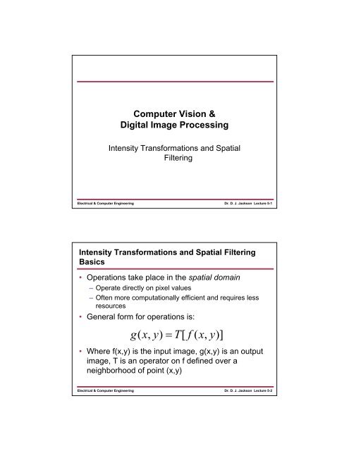
Computer Vision &Digital Image ProcessingIntensity Transformations and SpatialFilteringElectrical & Computer EngineeringDr. D. J. Jackson Lecture 5-1Intensity Transformations and Spatial FilteringBasics• Operations take place in the spatial domain– Operate directly on pixel values– Often more computationally efficient and requires lessresources• General form for operations is:g ( x,y)= T[f ( x,y)]• Where f(x,y) is the input image, g(x,y) is an outputimage, T is an operator on f defined over aneighborhood of point (x,y)Electrical & Computer EngineeringDr. D. J. Jackson Lecture 5-2

Intensity Transformations and Spatial FilteringBasics (continued)• The operator can apply to asingle image or to a set ofimages• The point (x,y) shown is anarbitrary point in the image• The region containing thepoint is a neighborhood of(x,y)• Typically the neighborhoodis rectangular, centered on(x,y) and is much smallerthan the imageElectrical & Computer EngineeringDr. D. J. Jackson Lecture 5-3Intensity Transformations and Spatial FilteringBasics (continued)• Spatial filtering– Generally involves operations over the entire image– Operations take place involving pixels within aneighborhood of a point of interest (x,y)– Also involves a predefined operation called a spatial filter– The spatial filter is also commonly referred to as:• Spatial mask• Kernel• Template• WindowElectrical & Computer EngineeringDr. D. J. Jackson Lecture 5-4

Point Processing• The smallest neighborhood of a pixel is 1×1 in size• Here, g depends only on the value of f at (x,y)• T becomes an intensity transformation function ofthe forms = T (r)• where s and r represent the intensity of g and f atany point (x,y)• Also called a gray-level or mapping functionElectrical & Computer EngineeringDr. D. J. Jackson Lecture 5-5Intensity Transformation ExampleElectrical & Computer EngineeringDr. D. J. Jackson Lecture 5-6

Some Basic Intensity Transformation Functions• Here, T is a transformation that maps a pixel value rinto a pixel value s• Since we are concerned with digital data, thetransformation can generally be implemented with asimple lookup table• Three basic types of transformations– Linear (negative and identity transformations)– Logarithmic (log and inverse-log transformations)– Power-law (n th power and n th root transformations)Electrical & Computer EngineeringDr. D. J. Jackson Lecture 5-7General Form for Basic Intensity TransformationsElectrical & Computer EngineeringDr. D. J. Jackson Lecture 5-8

Image Negatives• The negative of an image with intensity levels in the range[0,L-1] can be described by:s = L −1−rElectrical & Computer EngineeringDr. D. J. Jackson Lecture 5-9Log Transformations• General form:s = c log( 1+r)• c is a constant and r≥0• Maps a narrow range of low intensity values in input to awider output range• The opposite is true for high intensity input values• Compresses the dynamic range of images with largevariations in pixel valuesElectrical & Computer EngineeringDr. D. J. Jackson Lecture 5-10

Log Transformation Example• A plot (image) of the Fourier Spectrum is enhanced usually has a fairlylarge dynamic range• The image can be enhanced by applying the log transformationElectrical & Computer EngineeringDr. D. J. Jackson Lecture 5-11Power-Law (Gamma) Transformations• Basic formγs = cr• Where c and γ are positive constants• Power-law curves with fractional values of γ map anarrow range of dark input values to a wider rangeof output values• The opposite is true for higher values of input levels• There exists a family of possible transformationcurves by varying γElectrical & Computer EngineeringDr. D. J. Jackson Lecture 5-12

Power-Law Transformation CurvesElectrical & Computer EngineeringDr. D. J. Jackson Lecture 5-13Gamma Correction• Many devices used for image capture, display andprinting respond according to a power law• The exponent in the power-law equation is referredto as gamma• The process of correcting for the power-lawresponse is referred to as gamma correction• Example:– CRT devices have an intensity-to-voltage response that isa power function (exponents typically range from 1.8-2.5)– Gamma correction in this case could be achieved byapplying the transformation s=r 1/2.5 =r 0.4Electrical & Computer EngineeringDr. D. J. Jackson Lecture 5-14

Gamma Correction ExampleElectrical & Computer EngineeringDr. D. J. Jackson Lecture 5-15Gamma Correction (MRI Example)Electrical & Computer EngineeringDr. D. J. Jackson Lecture 5-16

Gamma Correction (Aerial Example)Electrical & Computer EngineeringDr. D. J. Jackson Lecture 5-17Piecewise-Linear Transformations• Piecewise functions can be arbitrarily complex• A disadvantage is that their specification requiressignificant user input• Example functions– Contrast stretching– Intensity-level slicing– Bit-plane slicingElectrical & Computer EngineeringDr. D. J. Jackson Lecture 5-18

Contrast Stretching• Contrast stretchingexpands the range ofintensity levels in an imageso it spans a given (full)intensity range• Control points (r 1 ,s 1 ) and(r 2 ,s 2 ) control the shape ofthe transform T(r)• r 1 =r 2 , s 1 =0 and s 2 =L-1yields a thresholdingfunctionElectrical & Computer EngineeringDr. D. J. Jackson Lecture 5-19Intensity-level Slicing• Used to highlight a specific range of intensities in an image that might beof interest• Two common approaches– Set all pixel values within a range of interest to one value (white) and allothers to another value (black)• Produces a binary image– Brighten (or darken) pixel values in a range of interest and leave all othersunchangedElectrical & Computer EngineeringDr. D. J. Jackson Lecture 5-20

Intensity-level Slicing (Angiogram Example)Electrical & Computer EngineeringDr. D. J. Jackson Lecture 5-21Bit-plane Slicing• Pixels are digital valuescomposed of bits• For example, a pixel in a256-level gray-scale imageis comprised of 8 bits• We can highlight thecontribution made to totalimage appearance byspecific bits• For example, we candisplay an image that onlyshows the contribution of aspecific bit planeElectrical & Computer EngineeringDr. D. J. Jackson Lecture 5-22

Bit-plane Slicing (Example)Electrical & Computer EngineeringDr. D. J. Jackson Lecture 5-23Bit-plane Slicing (continued)• Bit-plane slicing is useful in– Determining the number of bits necessary to quantize an image– Image compressionElectrical & Computer EngineeringDr. D. J. Jackson Lecture 5-24