Elliptic Modular Forms and Their Applications - Up To

Secretariat, and the resources available for ASEAN purposes. Accordingly, we directedthe ASEAN Senior Officials Meeting, the ASEAN Standing Committee and the ASEANSecretariat to work thoroughly on these matters and report to us at the earliestopportunity. We agreed to submit our views on the AEC to the 9 th ASEAN Summit in Baliin October 2003.10. We reviewed the Hanoi Plan of Action and agreed that the next Plan of Action shouldfocus on regional economic integration, while further narrowing the development gapwithin the region.ASEAN Tourism Agreement11. We reiterated our gratification over the signing by ASEAN’s leaders of the ASEANTourism Agreement (ATA) in Phnom Penh on 4 November 2002. Stressing the greatimportance of tourism to the development of our countries and noting that theimplementation of the ATA was the responsibility of various national agencies and ASEANbodies, we called for the early negotiation and conclusion of the agreements and otherinstruments necessary for the realization of the ATA’s purposes. We directed the ASEANStanding Committee and the ASEAN Secretariat, working together with the ASEANTourism Ministers and the National Tourism Organizations, to support this task. We calledon the developed countries to refrain from indiscriminately issuing travel advisories thatadversely affect trade and tourism in the region.Initiative for ASEAN Integration and the Mekong Basin12. We reaffirmed the critical political and economic significance of IAI in narrowing thedevelopment gap in ASEAN and strengthening the competitiveness of ASEAN as a whole.In this connection, we called for closer coordination among ASEAN bodies to accelerateactivities within the framework of the IAI and the Ha Noi Declaration on Narrowing theDevelopment Gap for closer ASEAN Integration. Recalling that the 8 th ASEAN Summithad approved the Work Plan for the Initiative for ASEAN Integration as a priority forASEAN, we were gratified by the efforts of the member-countries to implement the WorkPlan. Noting that the newer members had incorporated several elements of the IAI in theirnational policies and national development plans, we encouraged the internationalcommunity to extend concrete support to the projects embodied in the IAI Work Plan. Inthe long run, an integrated ASEAN with open markets would serve the economic interestsof ASEAN as well as its trading partners.13. We reviewed ASEAN-China cooperation on the development of the Mekong Basin withinthe ASEAN Mekong Basin Development Cooperation (AMBDC) framework. We reiteratedour call on Japan and the Republic of Korea to consider participating in the core group ofthe AMBDC, and the international community and international financial institutions tosupport the completion of the Singapore-Kunming Rail Link, specifically the construction ofthe missing segments of this project. Recalling the first GMS summit in Phnom Penh on 3November 2002, we expressed our appreciation for the Greater Mekong Sub-regionprogram of the Asian Development Bank. We urged that the various programs for thedevelopment of the Mekong Basin be undertaken in close coordination to ensure theequitable and sustainable development of the basin, taking into account the interests of allcountries, the concerns of the downstream countries, and the protection of theenvironment.Sub-Regional Growth Areas

Elliptic Modular Forms and Their Applications 5( ) az + bf= (cz + d) k f(z) (2)cz + dfor all z ∈ H and all ( abcd)∈ Γ1 ; conversely, given a function f : H → C satisfying(2), we can define a funcion on lattices, homogeneous of degree −k withrespect to homotheties, by F (Z.ω 1 + Z.ω 2 )=ω2 −k f(ω 1/ω 2 ). As with modularfunctions, there is a standard convention: when the word “modular form” (onsome discrete subgroup Γ of SL(2, R)) is used with no further adjectives, onegenerally means “holomorphic modular form”, i.e., a function f on H satisfying(2)forall( abcd)∈ Γ which is holomorphic in H and of subexponentialgrowth at infinity (i.e., f satisfies the same estimate as above, but now forall rather than some C>0). This growth condition, which corresponds toholomorphy at the cusps in a sense which we do not explain now, implies thatthe growth at infinity is in fact polynomial; more precisely, f automaticallysatisfies f(z) =O(1) as y →∞and f(x + iy) =O(y −k ) as y → 0. Wedenoteby M k (Γ ) the space of holomorphic modular forms of weight k on Γ .Aswewill see in detail for Γ = Γ 1 , this space is finite-dimensional, effectively computablefor all k, and zero for k

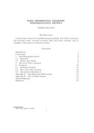
6 D. ZagierThe group Γ 1 is generated by the two elements T = ( ) (1101 and S = 0 1− 10),with the relations S 2 =(ST) 3 =1. The actions of S and T on H are given byS : z ↦→ −1/z , T : z ↦→ z +1.Therefore f is a modular form of weight k on Γ 1 precisely when f is periodicwith period 1 and satisfies the single further functional equationf ( −1/z ) = z k f(z) (z ∈ H) . (4)If we know the value of a modular form f on some group Γ at one pointz ∈ H, then equation (2) tells us the value at all points in the same Γ 1 -orbitas z. So to be able to completely determine f it is enough to know the value atone point from each orbit. This leads to the concept of a fundamental domainfor Γ , namely an open subset F⊂H such that no two distinct points of Fare equivalent under the action of Γ and every point z ∈ H is Γ -equivalent tosome point in the closure F of F.Proposition 1. The setF 1 = { }z ∈ H | |z| > 1, |R(z)| < 1 2is a fundamental domain for the full modular group Γ 1 . (See Fig. 1A.)Proof. Take a point z ∈ H. Then{mz + n | m, n ∈ Z} is a lattice in C.Every lattice has a point different from the origin of minimal modulus. Letcz + d be such a point. The integers c, d must be relatively prime (otherwisewe could divide cz + d by an integer to get a new point in the lattice of evensmaller modulus). So there are integers a and b such that γ 1 = ( abcd)∈ Γ1 .Bythe transformation property (1) for the imaginary part y = I(z) we get thatI(γ 1 z) is a maximal member of {I(γz) | γ ∈ Γ 1 }.Setz ∗ = T n γ 1 z = γ 1 z + n,Fig. 1. The standard fundamental domain for Γ 1 and its neighbors

Elliptic Modular Forms and Their Applications 7where n is such that |R(z ∗ )|≤ 1 2 . We cannot have |z∗ | < 1, because thenwe would have I(−1/z ∗ ) = I(z ∗ )/|z ∗ | 2 > I(z ∗ ) by (1), contradicting themaximality of I(z ∗ ).Soz ∗ ∈ F 1 ,andz is equivalent under Γ 1 to z ∗ .Now suppose that we had two Γ 1 -equivalent points z 1 and z 2 = γz 1 in F 1 ,with γ ≠ ±1. Thisγ cannot be of the form T n since this would contradictthe condition |R(z 1 )|, |R(z 2 )| < 1 2 ,soγ = ( abcd)with c ≠ 0.NotethatI(z) > √ 3/2 for all z ∈F 1 . Hence from (1) we get√32< I(z 2 ) =I(z 1 )|cz 1 + d| 2 ≤ I(z 1)c 2 I(z 1 ) 2 < 2c 2√ 3 ,which can only be satisfied if c = ±1. Without loss of generality we mayassume that Iz 1 ≤ Iz 2 .But|±z 1 +d| ≥|z 1 | > 1, and this gives a contradictionwith the transformation property (1).Remarks. 1. The points on the borders of the fundamental region are Γ 1 -equivalent as follows: First, the points on the two lines R(z) =± 1 2are equivalentby the action of T : z ↦→ z +1. Secondly, the points on the left and righthalves of the arc |z| =1are equivalent under the action of S : z ↦→ −1/z. Infact, these are the only equivalences for the points on the boundary. For thisreason we define ˜F 1 to be the semi-closure of F 1 where we have added only theboundary points with non-positive real part (see Fig. 1B). Then every pointof H is Γ 1 -equivalent to a unique point of ˜F 1 , i.e., ˜F 1 is a strict fundamentaldomain for the action of Γ 1 . (But terminology varies, and many people usethe words “fundamental domain” for the strict fundamental domain or for itsclosure, rather than for the interior.)2. The description of the fundamental domain F 1 also implies the abovementionedfact that Γ 1 (or Γ 1 ) is generated by S and T . Indeed, by the verydefinition of a fundamental domain we know that F 1 and its translates γF 1 byelements γ of Γ 1 cover H, disjointly except for their overlapping boundaries(a so-called “tesselation” of the upper half-plane). The neighbors of F 1 areT −1 F 1 , SF 1 and T F 1 (see Fig. 1C), so one passes from any translate γF 1of F 1 to one of its three neighbors by applying γSγ −1 or γT ±1 γ −1 .Inparticular,if the element γ describing the passage from F 1 to a given translatedfundamental domain F 1 ′ = γF 1 canbewrittenasawordinS and T ,thenso can the element of Γ 1 which describes the motion from F 1 to any of theneighbors of F 1 ′ . Therefore by moving from neighbor to neighbor across thewhole upper half-plane we see inductively that this property holds for everyγ ∈ Γ 1 , as asserted. More generally, one sees that if one has given a fundamentaldomain F for any discrete group Γ , then the elements of Γ which identifyin pairs the sides of F always generate Γ .♠Finiteness of Class NumbersLet D be a negative discriminant, i.e., a negative integer which is congruentto 0 or 1 modulo 4. We consider binary quadratic forms of the form Q(x, y) =

8 D. ZagierAx 2 + Bxy + Cy 2 with A, B, C ∈ Z and B 2 − 4AC = D. Such a form isdefinite (i.e., Q(x, y) ≠0for non-zero (x, y) ∈ R 2 ) and hence has a fixed sign,which we take to be positive. (This is equivalent to A>0.) We also assumethat Q is primitive, i.e., that gcd(A, B, C) = 1.DenotebyQ D the set ofthese forms. The group Γ 1 (or indeed Γ 1 )actsonQ D by Q ↦→ Q ◦ γ, where(Q ◦ γ)(x, y) =Q(ax + by, cx + dy) for γ = ± ( abcd)∈ Γ1 . We claim that thenumber of equivalence classes under this action is finite. This number, calledthe class number of D and denoted h(D), also has an interpretation as thenumber of ideal classes (either for the ring of integers or, if D is a non-trivialsquare multiple of some other discriminant, for a non-maximal order) in theimaginary quadratic field Q( √ D), so this claim is a special case – historicallythe first one, treated in detail in Gauss’s Disquisitiones Arithmeticae –ofthe general theorem that the number of ideal classes in any number field isfinite. To prove it, we observe that we can associate to any Q ∈ Q D theunique root z Q =(−B + √ √ √D)/2A of Q(z, 1) = 0 in the upper half-plane (hereD =+i |D| by definition and A>0 by assumption). One checks easilythat z Q◦γ = γ −1 (z Q ) for any γ ∈ Γ 1 ,soeachΓ 1 -equivalence class of formsQ ∈ Q D has a unique representative belonging to the setQ redD = { [A, B, C] ∈ Q D |−A

Elliptic Modular Forms and Their Applications 9z ∈ H which have a non-trivial stabilizer for the image of Γ in PSL(2, R)) aresingular and also that Γ \H is not compact, but has to be compactified by theaddition of one or more further points called cusps. We explain this for thecase Γ = Γ 1 .In §1.2 we identified the quotient space Γ 1 \H as a set with the semiclosure˜F 1 of F 1 and as a topological space with the quotient of F 1 obtainedby identifying the opposite sides (lines R(z) =± 1 2or halves of the arc |z| =1)of the boundary ∂F 1 . For a generic point of ˜F 1 the stabilizer subgroup of Γ 1is trivial. But the two points ω = 1 2 (−1+i√ 3) = e 2πi/3 and i are stabilizedby the cyclic subgroups of order 3 and 2 generated by ST and S respectively.This means that in the quotient manifold Γ 1 \H, ω and i are singular. (Froma metric point of view, they have neighborhoods which are not discs, butquotients of a disc by these cyclic subgroups, with total angle 120 ◦ or 180 ◦instead of 360 ◦ .) If we define an integer n P for every P ∈ Γ 1 \H as the orderof the stabilizer in Γ 1 of any point in H representing P ,thenn P equals 2or 3 if P is Γ 1 -equivalent to i or ω and n P =1otherwise. We also have toconsider the compactified quotient Γ 1 \H obtained by adding a point at infinity(“cusp”) to Γ 1 \H. More precisely, for Y > 1 the image in Γ 1 \H of the part of Habove the line I(z) =Y can be identified via q = e 2πiz with the punctureddisc 0

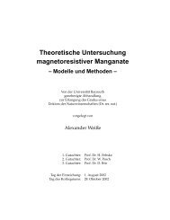
10 D. ZagierFig. 2. The zeros of a modular form(they consist of a full circle if P is an interior point of F 1 and of two half-circlesif P corresponds to a boundary point of F 1 different from ω, ω +1or i), andtotal angle π or 2π/3 if P ∼ i or ω. The corresponding contributions to theintegral are as follows. The two vertical lines together give 0, because f takeson the same value on both and the orientations are opposite. The horizontalline from − 1 2 +iY to 1 2 +iY gives a contribution 2πi ord ∞(f), because d(log f)is the sum of ord ∞ (f) dq/q and a function of q which is holomorphic at 0,and this integral corresponds to an integral around a small circle |q| = e −2πYaround q =0. The integral on the boundary of the deleted ε-neighborhood ofa zero P of f contributes 2πi ord P (f) if n P =1by Cauchy’s theorem, becauseord P (f) is the residue of d(log f(z)) at z = P , while for n P > 1 we mustdivide by n P because we are only integrating over one-half or one-third of thefull circle around P . Finally, the integral along the bottom arc contributesπik/6, as we see by breaking up this arc into its left and right halves andapplying the formula d log f(Sz)=d log f(z)+kdz/z, which is a consequenceof the transformation equation (4). Combining all of these terms with theappropriate signs dictated by the orientation, we obtain (6). The details areleft to the reader.Corollary 1. The dimension of M k (Γ 1 ) is 0 for k

Elliptic Modular Forms and Their Applications 11combination f of them which vanishes in all P i , by linear algebra. But thenf ≡ 0 by the proposition, since m>k/12, sothef i are linearly dependent.Hence dim M k (Γ 1 ) ≤ m. Ifk ≡ 2 (mod 12) we can improve the estimate by 1by noticing that the only way to satisfy (6) is to have (at least) a simplezero∑at i and a double zero at ω (contributing a total of 1/2+2/3 =7/6 toordP (f)/n P ) together with k/12 − 7/6 =m − 1 further zeros, so that thesame argument now gives dim M k (Γ 1 ) ≤ m − 1.Corollary 2. The space M 12 (Γ 1 ) has dimension ≤ 2, andiff, g ∈ M 12 (Γ 1 )are linearly independent, then the map z ↦→ f(z)/g(z) gives an isomorphismfrom Γ 1 \H ∪{∞} to P 1 (C).Proof. The first statement is a special case of Corollary 1. Suppose that fand g are linearly independent elements of M 12 (Γ 1 ). For any (0, 0) ≠(λ, μ) ∈C 2 the modular form λf −μg of weight 12 has exactly one zero in Γ 1 \H∪{∞}by Proposition 2, so the modular function ψ = f/g takes on every value(μ : λ) ∈ P 1 (C) exactly once, as claimed.We will make an explicit choice of f, g and ψ in §2.4, after we have introducedthe “discriminant function” Δ(z) ∈ M 12 (Γ 1 ).The true interpretation of the factor 1/12 multiplying k in equation (6)is as 1/4π times the volume of Γ 1 \H, taken with respect to the hyperbolicmetric. We say only a few words about this, since these ideas will not beused again. To give a metric on a manifold is to specify the distance betweenany two sufficiently near points. The hyperbolic metric in H is definedby saying that the hyperbolic distance between two points in a small neighborhoodof a point z = x + iy ∈ H is very nearly 1/y times the Euclideandistance between them, so the volume element, which in Euclidean geometry isgiven by the 2-form dx dy, is given in hyperbolic geometry by dμ = y −2 dx dy.ThusVol ( ∫ ∫ 1/2(∫ ∞)dyΓ 1 \H) = dμ =√F 1 −1/2 1−x 2 y 2 dx=∫ 1/2−1/2∣dx∣∣∣1/2√ = arcsin(x) 1 − x2−1/2= π 3 .Now we can consider other discrete subgroups of SL(2, R) which have a fundamentaldomain of finite volume. (Such groups are usually called Fuchsiangroups of the first kind, and sometimes “lattices”, but we will reserve this latterterm for discrete cocompact subgroups of Euclidean spaces.) Examplesare the subgroups Γ ⊂ Γ 1 of finite index, for which the volume of Γ \H is π/3times the index of Γ in Γ 1 (or more precisely, of the image of Γ in PSL(2, R)in Γ 1 ). If Γ is any such group, then essentially the same proof as for Proposition2 shows that the number of Γ -inequivalent zeros of any non-zero

12 D. Zagiermodular form f ∈ M k (Γ ) equals k Vol(Γ \H)/4π, where just as in the caseof Γ 1 we must count the zeros at elliptic fixed points or cusps of Γ withappropriate multiplicities. The same argument as for Corollary 1 of Proposition2 then tells us M k (Γ ) is finite dimensional and gives an explicit upperbound:Proposition 3. Let Γ be a discrete subgroup of SL(2, R) for which Γ \H hasfinite volume V .Then dim M k (Γ ) ≤ kV +1 for all k ∈ Z.4πIn particular, we have M k (Γ )={0} for k2 and the discriminant function Δ(z) of weight 12,whose definition is closely connected to the non-modular Eisenstein seriesE 2 (z).2.1 Eisenstein Series and the Ring Structure of M ∗ (Γ 1 )There are two natural ways to introduce the Eisenstein series. For the first,we observe that the characteristic transformation equation (2) of a modular

Elliptic Modular Forms and Their Applications 13form can be written in the form f| k γ = f for γ ∈ Γ ,wheref| k γ : H → C isdefined by( ∣f ∣k g ) ( ) az + b(z) = (cz + d) −k fcz + d( )( abz ∈ C, g = ∈ SL(2, R) ) .cd(8)One checks easily that for fixed k ∈ Z, themapf ↦→ f| k g defines an operationof the group SL(2, R) (i.e., f| k (g 1 g 2 )=(f| k g 1 )| k g 2 for all g 1 ,g 2 ∈ SL(2, R))on the vector space of holomorphic functions in H having subexponentialor polynomial growth. The space M k (Γ ) of holomorphic modular forms ofweight k on a group Γ ⊂ SL(2, R) is then simply the subspace of this vectorspace fixed by Γ .If we have a linear action v ↦→ v|g of a finite group G on a vector space V ,then an obvious way to construct a G-invariant vector in V is to start withan arbitrary vector v 0 ∈ V and form the sum v = ∑ g∈G v 0|g (and to hopethat the result is non-zero). If the vector v 0 is invariant under some subgroupG 0 ⊂ G, then the vector v 0 |g depends only on the coset G 0 g ∈ G 0 \Gand we can form instead the smaller sum v = ∑ g∈G v 0\G 0|g, which again isG-invariant. If G is infinite, the same method sometimes applies, but we nowhave to be careful about convergence. If the vector v 0 is fixed by an infinitesubgroup G 0 of G, then this improves our chances because the sum over G 0 \Gis much smaller than a sum over all of G (and in any case ∑ g∈Gv|g has nochance of converging since every term occurs infinitely often). In the contextwhen G = Γ ⊂ SL(2, R) is a Fuchsian group (acting by | k )andv 0 arationalfunction, the modular forms obtained in this way are called Poincaréseries. An especially easy case is that when v 0 is the constant function “1”∑and Γ 0 = Γ ∞ , the stabilizer of the cusp at infinity. In this case the seriesΓ 1| ∞\Γ kγ is called an Eisenstein series.Let us look at this series more carefully when Γ = Γ 1 .Amatrix ( abcd)∈SL(2, R) sends ∞ to a/c, and hence belongs to the stabilizer of ∞ if and onlyif c =0.InΓ 1 these are the matrices ± ( 1 n01)with n ∈ Z, i.e., up to sign thematrices T n . We can assume that k is even (since there are no modular formsof odd weight on Γ 1 ) and hence work with Γ 1 = PSL(2, Z), inwhichcasethestabilizer Γ ∞ is the infinite cyclic group generated by T . If we multiply anarbitrary matrix γ = ( ) (abcd on the left by 1 n( 01), then the resulting matrix γ ′ =a+nc b+nd)c d has the same bottom row as γ.Conversely,ifγ ′ = ( )a ′ b ′c d ∈ Γ1 hasthe same bottom row as γ,thenfrom(a ′ −a)d−(b ′ −b)c =det(γ)−det(γ ′ )=0and (c, d) =1(the elements of any row or column of a matrix in SL(2, Z) arecoprime!) we see that a ′ − a = nc, b ′ − b = nd for some n ∈ Z, i.e., γ ′ = T n γ.Since every coprime pair of integers occurs as the bottom row of a matrix inSL(2, Z), these considerations give the formulaE k (z) =∑γ∈Γ ∞\Γ 11 ∣ ∣kγ =∑γ∈Γ ∞\Γ 11 ∣ ∣kγ = 1 2∑c, d∈Z(c,d) =11(cz + d) k (9)

14 D. Zagierfor the Eisenstein series (the factor 1 2arises because (c d) and (−c − d) givethe same element of Γ 1 \Γ 1 ). It is easy to see that this sum is absolutelyconvergent for k>2 (the number of pairs (c, d) with N ≤|cz + d| 2, z∈ H) , (10)where the sum is again absolutely and locally uniformly convergent for k>2,guaranteeing that G k ∈ M k (Γ 1 ). The modularity can also be seen directly bynoting that (G k | k γ)(z) = ∑ m,n (m′ z + n ′ ) −k where (m ′ ,n ′ )=(m, n)γ runsover the non-zero vectors of Z 2 {(0, 0)} as (m, n) does.In fact, the two functions (9) and (10) are proportional, as is easily seen:any non-zero vector (m, n) ∈ Z 2 can be written uniquely as r(c, d) with r (thegreatest common divisor of m and n) a positive integer and c and d coprimeintegers, soG k (z) = ζ(k) E k (z) , (11)where ζ(k) = ∑ r≥1 1/rk is the value at k of the Riemann zeta function. Itmay therefore seem pointless to have introduced both definitions. But in fact,this is not the case. First of all, each definition gives a distinct point of viewand has advantages in certain settings which are encountered at later pointsin the theory: the E k definition is better in contexts like the famous Rankin-Selberg method where one integrates the product of the Eisenstein series withanother modular form over a fundamental domain, while the G k definition isbetter for analytic calculations and for the Fourier development given in §2.2.

Elliptic Modular Forms and Their Applications 15Moreover, if one passes to other groups, then there are σ Eisenstein series ofeach type, where σ is the number of cusps, and, although they span the samevector space, they are not individually proportional. In fact, we will actuallywant to introduce a third normalizationG k (z) =(k − 1)!(2πi) k G k(z) (12)because, as we will see below, it has Fourier coefficients which are rationalnumbers (and even, with one exception, integers) and because it is a normalizedeigenfunction for the Hecke operators discussed in §4.As a first application, we can now determine the ring structure of M ∗ (Γ 1 )Proposition 4. The ring M ∗ (Γ 1 ) is freely generated by the modular forms E 4and E 6 .Corollary. The inequality (7) for the dimension of M k (Γ 1 ) is an equality forall even k ≥ 0.Proof. The essential point is to show that the modular forms E 4 (z) andE 6 (z) are algebraically independent. To see this, we first note that the formsE 4 (z) 3 and E 6 (z) 2 of weight 12 cannot be proportional. Indeed, if we hadE 6 (z) 2 = λE 4 (z) 3 for some (necessarily non-zero) constant λ, then themeromorphic modular form f(z) =E 6 (z)/E 4 (z) of weight 2 would satisfyf 2 = λE 4 (and also f 3 = λ −1 E 6 ) and would hence be holomorphic (a functionwhose square is holomorphic cannot have poles), contradicting the inequalitydim M 2 (Γ 1 ) ≤ 0 of Corollary 1 of Proposition 2. But any two modularforms f 1 and f 2 of the same weight which are not proportional are necessarilyalgebraically independent. Indeed, if P (X, Y ) is any polynomial in C[X, Y ]such that P (f 1 (z),f 2 (z)) ≡ 0, then by considering the weights we see thatP d (f 1 ,f 2 ) has to vanish identically for each homogeneous component P d of P .But P d (f 1 ,f 2 )/f2d = p(f 1/f 2 ) for some polynomial p(t) in one variable, andsince p has only finitely many roots we can only have P d (f 1 ,f 2 ) ≡ 0 if f 1 /f 2is a constant. It follows that E4 3 and E2 6 , and hence also E 4 and E 6 , are algebraicallyindependent. But then an easy calculation shows that the dimensionof the weight k part of the subring of M ∗ (Γ 1 ) which they generate equals theright-hand side of the inequality (7), so that the proposition and corollaryfollow from this inequality.2.2 Fourier Expansions of Eisenstein SeriesRecall from (3) that any modular form on Γ 1 has a Fourier expansion of theform ∑ ∞n=0 a nq n ,whereq = e 2πiz . The coefficients a n often contain interestingarithmetic information, and it is this that makes modular forms importantfor classical number theory. For the Eisenstein series, normalized by (12), thecoefficients are given by:

16 D. ZagierProposition 5. The Fourier expansion of the Eisenstein series G k (z)(k even,k>2) isG k (z) = − B ∞ k2k + ∑σ k−1 (n) q n , (13)n=1where B k is the kth Bernoulli number and where σ k−1 (n) for n ∈ N denotesthe sum of the (k − 1)st powers of the positive divisors of n.We∑recall that the Bernoulli numbers are defined by the generating function∞k=0 B kx k /k! =x/(e x − 1) and that the first values of B k (k>0 even) aregiven by B 2 = 1 6 , B 4 = − 1 30 , B 6 = 142 , B 8 = − 1 30 , B 10 = 5 66 , B 12 = − 6912730 ,and B 14 = 7 6 .Proof. A well known and easily proved identity of Euler states that∑n∈Z1z + n =πtan πz(z ∈ C \ Z), (14)where the sum on the left, which is not absolutely convergent, is to be interpretedas a Cauchy principal value ( = lim ∑ N−Mwhere M, N tend to infinitywith M − N bounded). The function on the right is periodic of period 1 andits Fourier expansion for z ∈ H is given byπtan πz= πcos πzsin πz= πi eπiz + e −πiz 1+qe πiz = −πi− e−πiz 1 − q = −2πi ( 12 + ∞ ∑r=1q r ),where q = e 2πiz . Substitute this into (14), differentiate k − 1 times and divideby (−1) k−1 (k − 1)! to get∑ 1(z + n) k = (−1)k−1 d k−1 ( ) π∞∑(k − 1)! dz k−1 = (−2πi)k r k−1 q rtan πz (k − 1)!n∈Zr=1(k ≥ 2, z∈ H) ,an identity known as Lipschitz’s formula. Now the Fourier expansion of G k(k >2 even) is obtained immediately by splitting up the sum in (10) into theterms with m =0and those with m ≠0:G k (z) = 1 2∑n∈Zn≠01n k + 1 2= ζ(k) + (2πi)k(k − 1)!= (2πi)k(k − 1)!∑m, n∈Zm≠0(− B k2k +∞∑m=1 r=1∑∞1∞(mz + n) k = ∑n=1∞∑r k−1 q mrσ k−1 (n) q n ),n=11∞n k + ∑∞∑m=1 n=−∞1(mz + n) kwhere in the last line we have used Euler’s evaluation of ζ(k) (k >0 even) interms of Bernoulli numbers. The result follows.

Elliptic Modular Forms and Their Applications 19in this weight we can simply define the Eisenstein series G 2 , G 2 and E 2 byequations (13), (12), and (11), respectively, i.e.,G 2 (z) = − 1∞ 24 + ∑σ 1 (n) q n = − 1 24 + q +3q2 +4q 3 +7q 4 +6q 5 + ··· ,n=1G 2 (z) = −4π 2 G 2 (z) , E 2 (z) = 6 π 2 G 2(z) = 1 − 24q − 72q 2 − ··· .(17)Moreover, the same proof as for Proposition 5 still shows that G 2 (z) is givenby the expression (10), if we agree to carry out the summation over n firstandthenoverm :G 2 (z) = 1 2∑n≠01n 2 + 1 ∑2∑m≠0 n∈Z1(mz + n) 2 . (18)The only difference is that, because of the non-absolute convergence of thedouble series, we can no longer interchange the order of summation to getthe modular transformation equation G 2 (−1/z) =z 2 G 2 (z). (TheequationG 2 (z +1)=G 2 (z), of course, still holds just as for higher weights.) Nevertheless,the function G 2 (z) and its multiples E 2 (z) and G 2 (z) do have somemodular properties and, as we will see later, these are important for manyapplications.Proposition 6. For z ∈ H and ( abcd)∈ SL(2, Z) we have( ) az + bG 2 = (cz + d) 2 G 2 (z) − πic(cz + d) . (19)cz + dProof. There are many ways to prove this. We sketch one, due to Hecke, sincethe method is useful in many other situations. The series (10) for k = 2does∑not converge absolutely, but it is just at the edge of convergence, sincem,n |mz + n|−λ converges for any real number λ>2. We therefore modifythe sum slightly by introducingG 2,ε (z) = 1 ∑′ 12 (mz + n) 2 |mz + n| 2ε (z ∈ H, ε>0) . (20)m, n(Here ∑ ′means that the value (m, n) = (0, 0) is to be omitted fromthe ( summation.) The new series converges absolutely and transforms byG az+b)2,ε cz+d = (cz + d) 2 |cz + d| 2ε G 2,ε (z). We claim that lim G 2,ε (z) existsε→0and equals G 2 (z) − π/2y, wherey = I(z). It follows that each of the threenon-holomorphic functionsG ∗ 2 (z) = G 2(z) − π 2y , E∗ 2 (z) = E 2(z) − 3πy , G∗ 2 (z) = G 2(z) + 18πy(21)transforms like a modular form of weight 2, and from this one easily deducesthe transformation equation (19) and its analogues for E 2 and G 2 .Toprove

20 D. Zagierthe claim, we define a function I ε by∫ ∞dt(I ε (z) =z ∈ H, ε>−1(z + t) 2 |z + t| 2).2ε−∞Then for ε>0 we can write∞∑∞∑ 1G 2,ε − I ε (mz) =n 2+2εm=1n=1∞∑ ∞∑[∫1n+1]+(mz + n) 2 |mz + n| 2ε − dt(mz + t) 2 |mz + t| 2ε .m=1 n=−∞Both sums on the right converge absolutely and locally uniformly for ε>− 1 2(the second one because the expression in square brackets is O ( |mz+n| −3−2ε)by the mean-value theorem, which tells us that f(t) − f(n) for any differentiablefunction f is bounded in n ≤ t ≤ n +1 by max n≤u≤n+1 |f ′ (u)|), sothe limit of the expression on the right as ε → 0 exists and can be obtainedsimply by putting ε =0in each term, where it reduces to G 2 (z) by (18). Onthe other hand, for ε>− 1 2we have∫ ∞dtI ε (x + iy) =−∞ (x + t + iy) 2 ((x + t) 2 + y 2 ) ε∫ ∞dt=(t + iy) 2 (t 2 + y 2 ) ε = I(ε)y 1+2ε ,−∞where I(ε) = ∫ ∞−∞ (t+i)−2 (t 2 +1) −ε dt ,so ∑ ∞m=1 I ε(mz) =I(ε)ζ(1+2ε)/y 1+2εfor ε>0. Finally, we have I(0) = 0 (obvious),∫ ∞I ′ log(t 2 ( )∣+1) 1 + log(t 2 +1)∣∣∣∞(0) = −−∞ (t + i) 2 dt =− tan −1 t = − π,t + i−∞and ζ(1+2ε) = 1 2ε +O(1), so the product I(ε)ζ(1+2ε)/y1+2ε tends to −π/2yas ε → 0. The claim follows.Remark. The transformation equation (18) says that G 2 is an example of whatis called a quasimodular form, while the functions G ∗ 2 , E∗ 2 and G∗ 2 defined in(21) are so-called almost holomorphic modular forms of weight 2. We willreturn to this topic in Section 5.2.4 The Discriminant Function and Cusp FormsFor z ∈ H we define the discriminant function Δ(z) by the formulanΔ(z) = e 2πiz∞∏n=1(1 − e2πinz ) 24. (22)

Elliptic Modular Forms and Their Applications 21(The name comes from the connection with the discriminant of the ellipticcurve E z = C/(Z.z + Z.1), but we will not discuss this here.) Since |e 2πiz | < 1for z ∈ H, the terms of the infinite product are all non-zero and tend exponentiallyrapidly to 1, so the product converges everywhere and defines a holomorphicand everywhere non-zero function in the upper half-plane. This functionturns out to be a modular form and plays a special role in the entire theory.Proposition 7. The function Δ(z) is a modular form of weight 12 on SL(2, Z).Proof. Since Δ(z) ≠0, we can consider its logarithmic derivative. We find12πid∞dz log Δ(z) =1−24 ∑n=1ne 2πinz∞1 − e 2πinz =1−24 ∑m=1σ 1 (m) e 2πimz = E 2 (z) ,e 2πinzwhere the second equality follows by expandingas a geometric1 − e2πinz series ∑ ∞r=1 e2πirnz and interchanging the order of summation, and the thirdequality from the definition of E 2 (z) in (17). Now from the transformationequation for E 2 (obtained by comparing (19) and(11)) we find( (1 d Δ az+b) )( )2πi dz log cz+d1 az + b(cz + d) 12 =Δ(z) (cz + d) 2 E 2 − 12 ccz + d 2πi cz + d − E 2(z)=0.In other words, (Δ| 12 γ)(z) =C(γ)Δ(z) for all z ∈ H and all γ ∈ Γ 1 ,whereC(γ) is a non-zero complex number depending only on γ, andwhereΔ| 12 γ isdefined as in (8). It remains to show that C(γ) =1for all γ. ButC : Γ 1 → C ∗is a homomorphism because Δ ↦→ Δ| 12 γ is a group action, so it suffices tocheck this for the generators T = ( ) (1101 and S = 0 −1)1 0 of Γ1 . The first isobvious since Δ(z) is a power series in e 2πiz and hence periodic of period 1,while the second follows by substituting z = i into the equation Δ(−1/z) =C(S) z 12 Δ(z) and noting that Δ(i) ≠0.Let us look at this function Δ(z) more carefully. We know from Corollary 1to Proposition 2 that the space M 12 (Γ 1 ) has dimension at most 2, so Δ(z)must be a linear combination of the two functions E 4 (z) 3 and E 6 (z) 2 .Fromthe Fourier expansions E4 3 = 1 + 720q + ···, E 6 (z) 2 =1− 1008q + ··· andΔ(z) =q + ··· we see that this relation is given byΔ(z) = 1 (E4 (z) 3 − E 6 (z) 2) . (23)1728This identity permits us to give another, more explicit, version of the fact thatevery modular form on Γ 1 is a polynomial in E 4 and E 6 (Proposition 4). Indeed,let f(z) be a modular form of arbitrary even weight k ≥ 4, withFourierexpansion as in (3). Choose integers a, b ≥ 0 with 4a +6b = k (thisisalways

22 D. Zagierpossible) and set h(z) = ( f(z)−a 0 E 4 (z) a E 6 (z) b) /Δ(z). This function is holomorphicin H (because Δ(z) ≠0) and also at infinity (because f − a 0 E a 4 Eb 6has a Fourier expansion with no constant term and the Fourier expansion ofΔ begins with q), so it is a modular form of weight k − 12. By induction onthe weight, h is a polynomial in E 4 and E 6 ,andthenfromf = a 0 E a 4 Eb 6 +Δhand (23) we see that f also is.In the above argument we used that Δ(z) has a Fourier expansion beginningq+O(q 2 ) and that Δ(z) is never zero in the upper half-plane. We deducedboth facts from the product expansion (22), but it is perhaps worth notingthat this is not necessary: if we were simply to define Δ(z) by equation (23),then the fact that its Fourier expansion begins with q would follow from theknowledge of the first two Fourier coefficients of E 4 and E 6 , and the fact thatit never vanishes in H would then follow from Proposition 2 because the totalnumber k/12 = 1 of Γ 1 -inequivalent zeros of Δ is completely accounted forby the first-order zero at infinity.We can now make the concrete normalization of the isomorphism betweenΓ 1 \H and P 1 (C) mentioned after Corollary 2 of Proposition 2. In the notationof that proposition, choose f(z) =E 4 (z) 3 and g(z) =Δ(z). Their quotient isthen the modular functionj(z) = E 4(z) 3Δ(z)= q −1 + 744 + 196884 q + 21493760 q 2 + ··· ,called the modular invariant. SinceΔ(z) ≠0for z ∈ H, this function is finitein H and defines an isomorphism from Γ 1 \H to C as well as from Γ 1 \H toP 1 (C).The next (and most interesting) remarks about Δ(z) concern its Fourierexpansion. By multiplying out the product in (22) we obtain the expansion∞∏ (Δ(z) = q 1 − q n ) 24 =n=1∞∑τ(n) q n (24)n=1where q = e 2πiz as usual (this is the last time we will repeat this!) and thecoefficients τ(n) are certain integers, the first values being given by the tablen 1 2 3 4 5 6 7 8 9 10τ(n) 1 −24 252 −1472 4830 −6048 −16744 84480 −113643 −115920Ramanujan calculated the first 30 values of τ(n) in 1915 and observed severalremarkable properties, notably the multiplicativity property that τ(pq) =τ(p)τ(q) if p and q are distinct primes (e.g., −6048 = −24 · 252 for p =2,q =3)andτ(p 2 )=τ(p) 2 − p 11 if p is prime (e.g., −1472 = (−24) 2 − 2048 forp =2). This was proved by Mordell the next year and later generalized byHecke to the theory of Hecke operators, which we will discuss in §4.Ramanujan also observed that |τ(p)| was bounded by 2p 5√ p for primesp

Elliptic Modular Forms and Their Applications 23to be immeasurably deeper than the assertion about multiplicativity and wasonly proved in 1974 by Deligne as a consequence of his proof of the famous Weilconjectures (and of his previous, also very deep, proof that these conjecturesimplied Ramanujan’s). However, the weaker inequality |τ(p)| ≤Cp 6 with someeffective constant C>0 is much easier and was proved in the 1930’s by Hecke.We reproduce Hecke’s proof, since it is simple. In fact, the proof applies toa much more general class of modular forms. Let us call a modular form on Γ 1a cusp form if the constant term a 0 in the Fourier expansion (3) is zero. Sincethe constant term of the Eisenstein series G k (z) is non-zero, any modular formcan be written uniquely as a linear combination of an Eisenstein series anda cusp form of the same weight. For the former the Fourier coefficients aregiven by (13) and grow like n k−1 (since n k−1 ≤ σ k−1 (n) 0 depending only on f. Now the integral representation∫ 1a n = e 2πny f(x + iy) e −2πinx dx0for a n , valid for any y>0, show that |a n |≤cy −k/2 e 2πny .Takingy =1/n (or,optimally, y = k/4πn) gives the estimate of the proposition with C = ce 2π(or, optimally, C = c (4πe/k) k/2 ).Remark. The definition of cusp forms given above is actually valid only forthe full modular group Γ 1 or for other groups having only one cusp. In generalone must require the vanishing of the constant term of the Fourier expansionof f, suitably defined, at every cusp of the group Γ , in which case it againfollows that f can be estimated as in (25). Actually, it is easier to simply definecusp forms of weight k as modular forms for which y k/2 f(x + iy) is bounded,a definition which is equivalent but does not require the explicit knowledge ofthe Fourier expansion of the form at every cusp.♠ Congruences for τ (n)As a mini-application of the calculations of this and the preceding sectionswe prove two simple congruences for the Ramanujan tau-function defined by

24 D. Zagierequation (24). First of all, let us check directly that the coefficient τ(n) of q nof the function defined by (23) is integral for all n. (This fact is, of course,obvious from equation (22).) We haveΔ = (1 + 240A)3 − (1 − 504B) 21728= 5 A − B12+B +100A 2 −147B 2 +8000A 3(26)with A = ∑ ∞n=1 σ 3(n)q n and B = ∑ ∞n=1 σ 5(n)q n .Butσ 5 (n)−σ 3 (n) is divisibleby 12 for every n (because 12 divides d 5 − d 3 for every d), so (A − B)/12has integral coefficients. This gives the integrality of τ(n), and even a congruencemodulo 2. Indeed, we actually have σ 5 (n) ≡ σ 3 (n) (mod 24), becaused 3 (d 2 − 1) is divisible by 24 for every d, so (A − B)/12 has even coefficientsand (26) gives Δ ≡ B + B 2 (mod 2) or, recalling that ( ∑ ∑a n q n ) 2 ≡an q 2n (mod 2) for every power series ∑ a n q n with integral coefficients,τ(n) ≡ σ 5 (n)+σ 5 (n/2) (mod 2), whereσ 5 (n/2) is defined as 0 if 2 ∤ n. Butσ 5 (n), for any integer n, is congruent modulo 2 to the sum of the odd divisorsof n, and this is odd if and only if n is a square or twice a square, as onesees by writing n =2 s n 0 with n 0 odd and pairing the complementary divisorsof n 0 . It follows that σ 5 (n)+σ 5 (n/2) is odd if and only if n is an odd square,so we get the congruence:τ(n) ≡{1 (mod 2) if n is an odd square ,0 (mod 2) otherwise .(27)In a different direction, from dim M 12 (Γ 1 )=2we immediately deduce thelinear relationG 12 (z) = Δ(z) + 691 (E4 (z) 3+ E 6(z) 3 )156 720 1008and from this a famous congruence of Ramanujan,τ(n) ≡ σ 11 (n) (mod 691)(∀n ≥ 1), (28)where the “691” comes from the numerator of the constant term −B 12 /24 ofG 12 . ♥3 Theta SeriesIf Q is a positive definite integer-valued quadratic form in m variables, thenthere is an associated modular form of weight m/2, called the theta seriesof Q, whosenth Fourier coefficient for every integer n ≥ 0 is the number ofrepresentations of n by Q. This provides at the same time one of the mainconstructions of modular forms and one of the most important sources ofapplications of the theory. In 3.1 we consider unary theta series (m =1), while

Elliptic Modular Forms and Their Applications 25the general case is discussed in 3.2. The unary case is the most classical, goingback to Jacobi, and already has many applications. It is also the basis of thegeneral theory, because any quadratic form can be diagonalized over Q (i.e.,by passing to a suitable sublattice it becomes the direct sum of m quadraticforms in one variable).3.1 Jacobi’s Theta SeriesThe simplest theta series, corresponding to the unary (one-variable) quadraticform x ↦→ x 2 , is Jacobi’s theta functionθ(z) = ∑ n∈Zq n2 = 1 + 2q +2q 4 +2q 9 + ··· , (29)where z ∈ H and q = e 2πiz as usual. Its modular transformation propertiesare given as follows.Proposition 9. The function θ(z) satisfies the two functional equationsθ(z +1) = θ(z) ,θ( ) −14z=√2ziθ(z) (z ∈ H) . (30)Proof. The first equation in (30) is obvious since θ(z) depends only on q.For the second, we use the Poisson transformation formula. Recall that thisformula says that for any function f : R → C whichissmoothandsmallatinfinity, we have ∑ n∈Z f(n) =∑ ˜f(n), n∈Zwhere ˜f(y) = ∫ ∞−∞ e2πixy f(x) dx isthe Fourier transform of f. (Proof :thesum ∑ n∈Zf(n + x) is convergent anddefines a function g(x) which is periodic of period 1 and hence has a Fourierexpansion g(x) = ∑ n∈Z c ne 2πinx with c n = ∫ 10 g(x)e−2πinx dx = ˜f(−n),so ∑ n f(n) = g(0) = ∑ n c n = ∑ ˜f(−n) n= ∑ ˜f(n).) nApplying this tothe function f(x) =e −πtx2 ,wheret is a positive real number, and notingthat˜f(y) =∫ ∞−∞e −πtx2 +2πixy dx = e−πy2 /t√t∫ ∞−∞e −πu2 du = e−πy2 /t√t(substitution u = √ t (x − iy/t) followed by a shift of the path of integration),we obtain∞∑e −πn2 t= √ 1 ∑∞ e −πn2 /t(t >0) .tn=−∞n=−∞This proves the second equation in (30) for z = it/2 lying on the positiveimaginary axis, and the general case then follows by analytic continuation.

26 D. ZagierThe point is now that the two transformations z ↦→ z +1and z ↦→ −1/4zgenerate a subgroup of SL(2, R) which is commensurable with SL(2, Z), so(30) implies that the function θ(z) is a modular form of weight 1/2. (Wehave not defined modular forms of half-integral weight and will not discusstheir theory in these notes, but the reader can simply interpret this statementas saying that θ(z) 2 is a modular form of weight 1.) More specifically, forevery N ∈ N we have the “congruence subgroup” Γ 0 (N) ⊆ Γ 1 = SL(2, Z),consisting of matrices ( abcd)∈ Γ1 with c divisible by N, and the larger groupΓ 0 + (N) = 〈Γ (0(N),W N 〉 = Γ 0 (N) ∪ Γ 0 (N)W N ,whereW N = √ 1 0 −1)N N 0(“Fricke involution”) is an element of SL(2, R) of order 2 which normalizesΓ 0 (N). The group Γ 0 + (N) contains the elements T = ( 1101)and WN for anyN. In general they generate a subgroup of infinite index, so that to check themodularity of a given function it does not suffice to verify its behavior justfor z ↦→ z +1 and z ↦→ −1/N z, but for N =4(like for N =1!) they generatethe full group and this is sufficient. The proof is simple. Since WN 2 = −1, itissufficient to show that the two matrices T and ˜T = W 4 TW4 −1 = ( 1041)generatethe image of Γ 0 (4) in PSL(2, R), i.e., that any element γ = ( abcd)∈ Γ0 (4) is,up to sign, a word in T and ˜T .Nowa is odd, so |a| ≠2|b|. If|a| < 2|b|, theneither b+a or b−a is smaller than b in absolute value, so replacing γ by γ ·T ±1decreases a 2 + b 2 .If|a| > 2|b| ≠0, then either a +4b or a − 4b is smaller thana in absolute value, so replacing γ by γ · ˜T ±1 decreases a 2 + b 2 .Thuswecankeep multiplying γ on the right by powers of T and ˜T until b =0,atwhichpoint ±γ is a power of ˜T .Now, by the principle “a finite number of q-coefficients suffice” formulatedat the end of Section 1, the mere fact that θ(z) is a modular form isalready enough to let one prove non-trivial identities. (We enunciated theprinciple only in the case of forms of integral weight, but even without knowingthe details of the theory it is clear that it then also applies to halfintegralweight, since a space of modular forms of half-integral weight canbe mapped injectively into a space of modular forms of the next higher integralweight by multiplying by θ(z).) And indeed, with almost no effort weobtain proofs of two of the most famous results of number theory of the17th and 18th centuries, the theorems of Fermat and Lagrange about sums ofsquares.♠ Sums of Two and Four SquaresLet r 2 (n) = # { (a, b) ∈ Z 2 | a 2 + b 2 = n } be the number of representationsof an integer n ≥ 0 as a sum of two squares. Since θ(z) 2 =(∑a∈Z qa2 )(∑b∈Z qb2 ),weseethatr2 (n) is simply the coefficient of q n inθ(z) 2 . From Proposition 9 and the just-proved fact that Γ 0 (4) is generated by−Id 2 , T and ˜T , we find that the function θ(z) 2 is a “modular form of weight 1and character χ −4 on Γ 0 (4)” in the sense explained in the paragraph precedingequation (15), where χ −4 is the Dirichlet character modulo 4 defined by (15).

Elliptic Modular Forms and Their Applications 27Since the Eisenstein series G 1,χ−4 in (16) is also such a modular form, andsince the space of all such forms has dimension at most 1 by Proposition 3(because Γ 0 (4) has index 6 in SL(2, Z) and hence volume 2π), these two functionsmust be proportional. The proportionality factor is obviously 4, and weobtain:Proposition 10. Let n be a positive integer. Then the number of representationsof n as a sum of two squares is 4 times the sum of (−1) (d−1)/2 ,whered runs over the positive odd divisors of n .Corollary (Theorem of Fermat). Every prime number p ≡ 1(mod4)isasumoftwosquares.ProofofCorollary.We have r 2 (p) =4 ( 1+(−1) (p−1)/4) =8≠0.The same reasoning applies to other powers of θ. In particular, the numberr 4 (n) of representations of an integer n as a sum of four squares is the coefficientof q n in the modular form θ(z) 4 of weight 2 on Γ 0 (4), and the spaceof all such modular forms is at most two-dimensional by Proposition 3. Tofind a basis for it, we use the functions G 2 (z) and G ∗ 2 (z) defined in equations(17) and (21). We showed in §2.3 that the latter function transformswith respect to SL(2, Z) like a modular form of weight 2, and it follows easilythat the three functions G ∗ 2(z), G ∗ 2(2z) and G ∗ 2(4z) transform like modularforms of weight 2 on Γ 0 (4) (exercise!). Of course these three functions are notholomorphic, but since G ∗ 2 (z) differs from the holomorphic function G 2(z) by1/8πy, we see that the linear combinations G ∗ 2(z)−2G ∗ 2(2z) =G 2 (z)−2G 2 (2z)and G ∗ 2 (2z) − 2G∗ 2 (4z) =G 2(2z) − 2G 2 (4z) are holomorphic, and since theyare also linearly independent, they provide the desired basis for M 2 (Γ 0 (4)).Looking at the first two Fourier coefficients of θ(z) 4 =1+8q + ···, we findthat θ(z) 4 equals 8(G 2 (z)−2G 2 (2z))+16 (G 2 (2z)−2G 2 (4z)). Nowcomparingcoefficients of q n gives:Proposition 11. Let n be a positive integer. Then the number of representationsof n as a sum of four squares is 8 times the sum of the positive divisorsof n which are not multiples of 4.Corollary (Theorem of Lagrange). Every positive integer is a sum of foursquares. ♥For another simple application of the q-expansion principle, we introducetwo variants θ M (z) and θ F (z) (“M” and “F” for “male” and “female” or “minussign” and “fermionic”) of the function θ(z) by inserting signs or by shifting theindices by 1/2 in its definition:θ M (z) = ∑ n∈Z(−1) n q n2 = 1 − 2q +2q 4 − 2q 9 + ··· ,θ F (z) =∑n∈Z+1/2q n2 = 2q 1/4 +2q 9/4 +2q 25/4 + ··· .

28 D. ZagierThese are again modular forms of weight 1/2 on Γ 0 (4). With a little experimentation,we discover the identityθ(z) 4 = θ M (z) 4 + θ F (z) 4 (31)due to Jacobi, and by the q-expansion principle all we have to do to prove itis to verify the equality of a finite number of coefficients (here just one). Inthis particular example, though, there is also an easy combinatorial proof, leftas an exercise to the reader.The three theta series θ, θ M and θ F , in a slightly different guise andslightly different notation, play a role in many contexts, so we say a little moreabout them. As well as the subgroup Γ 0 (N) of Γ 1 , one also has the principalcongruence subgroup Γ (N) ={γ ∈ Γ 1 | γ ≡ Id 2 (mod N)} for every integerN ∈ N, which is more basic than Γ 0 (N) because it is a normal subgroup(the kernel of the map Γ 1 → SL(2, Z/N Z) given by reduction modulo N).Exceptionally, the group Γ 0 (4) is isomorphic to Γ (2), simply by conjugationby ( 2001)∈ GL(2, R), so that there is a bijection between modular forms onΓ 0 (4) of any weight and modular forms on Γ (2) of the same weight given byf(z) → f(z/2). In particular, our three theta functions correspond to threenew theta functionsθ 3 (z) = θ(z/2) , θ 4 (z) = θ M (z/2) , θ 2 (z) = θ F (z/2) (32)on Γ (2), and the relation (31) becomes θ2 4 + θ4 4 = θ4 3 . (Here the index “1” ismissing because the fourth member of the quartet, θ 1 (z) = ∑ (−1) n q (n+1/2)2 /2is identically zero, as one sees by sending n to −n − 1. Itmaylookoddthatone keeps a whole notation for the zero function. But in fact the functionsθ i (z) for 1 ≤ i ≤ 4 are just the “Thetanullwerte” or “theta zero-values” of thetwo-variable series θ i (z,u) = ∑ ε n q n2 /2 e 2πinu , where the sum is over Z orZ + 1 2and ε n is either 1 or (−1) n , none of which vanishes identically. Thefunctions θ i (z,u) play a basic role in the theory of elliptic functions and arealso the simplest example of Jacobi forms, a theory which is related to manyof the themes treated in these notes and is also important in connection withSiegel modular forms of degree 2 as discussed in Part III of this book.) Thequotient group Γ 1 /Γ (2) ∼ = SL(2, Z/2Z), which has order 6 and is isomorphicto the symmetric group S 3 on three symbols, acts as the latter on the modularforms θ i (z) 8 , while the fourth powers transform by⎛Θ(z) := ⎝ θ ⎞⎛2(z) 4− θ 3 (z) 4 ⎠ ⇒ Θ(z +1) = − ⎝ 100 ⎞001⎠ Θ(z),θ 4 (z) 4 010⎛(z −2 Θ − 1 )= − ⎝ 001⎞010⎠ Θ(z) .z100

Elliptic Modular Forms and Their Applications 29This illustrates the general principle that a modular form on a subgroup offinite index of the modular group Γ 1 can also be seen as a component ofa vector-valued modular form on Γ 1 itself. The full ring M ∗ (Γ (2)) of modularforms on Γ (2) is generated by the three components of Θ(z) (or by anytwo of them, since their sum is zero), while the subring M ∗ (Γ (2)) S3 =( M ∗ (Γ 1 ) is generated by the modular forms θ 2 (z) 8 + θ 3 (z) 8 + θ 4 (z) 8 andθ2 (z) 4 + θ 3 (z) 4)( θ 3 (z) 4 + θ 4 (z) 4)( θ 4 (z) 4 − θ 2 (z) 4) of weights 4 and 6 (whichare then equal to 2E 4 (z) and 2E 6 (z), respectively). Finally, we see that1256 θ 2(z) 8 θ 3 (z) 8 θ 4 (z) 8 is a cusp form of weight 12 on Γ 1 and is, in fact, equalto Δ(z).This last identity has an interesting consequence. Since Δ(z) is non-zerofor all z ∈ H, it follows that each of the three theta-functions θ i (z) has thesame property. (One can also see this by noting that the “visible” zero of θ 2 (z)at infinity accounts for all the zeros allowed by the formula discussed in §1.3,so that this function has no zeros at finite points, and then the same holds forθ 3 (z) and θ 4 (z) because they are related to θ 2 by a modular transformation.)This suggests that these three functions, or equivalently their Γ 0 (4)-versionsθ, θ M and θ F , might have a product expansion similar to that of the functionΔ(z), and indeed this is the case: we have the three identitiesθ(z) =η(2z) 5η(z) 2 η(4z) 2 ,θ M (z) = η(z)2η(2z) ,θ F (z) = 2 η(4z)2η(2z) , (33)where η(z) is the “Dedekind eta-function”∏∞η(z) = Δ(z) 1/24 = q 1/24 (1 − qn ) . (34)The proof of (33) is immediate by the usual q-expansion principle: we multiplythe identities out (writing, e.g., the first as θ(z)η(z) 2 η(4z) 2 = η(2z) 5 )andthenverify the equality of enough coefficients to account for all possible zeros ofa modular form of the corresponding weight. More efficiently, we can use ourknowledge of the transformation behavior of Δ(z) and hence of η(z) under Γ 1to see that the quotients on the right in (33) are finite at every cusp andhence, since they also have no poles in the upper half-plane, are holomorphicmodular forms of weight 1/2, after which the equality with the theta-functionson the left follows directly.More generally, one can ask when a quotient of products of eta-functionsis a holomorphic modular form. Since η(z) is non-zero in H, suchaquotientnever has finite zeros, and the only issue is whether the numerator vanishes toat least the same order as the denominator at each cusp. Based on extensivenumerical calculations, I formulated a general conjecture saying that thereare essentially only finitely many such products of any given weight, anda second explicit conjecture giving the complete list for weight 1/2 (i.e., whenthe number of η’s in the numerator is one bigger than in the denominator).Both conjectures were proved by Gerd Mersmann in a brilliant Master’s thesis.n=1

30 D. ZagierFor the weight 1/2 result, the meaning of “essentially” is that the productshould be primitive, i.e., it should have the form ∏ η(n i z) ai where the n iare positive integers with no common factor. (Otherwise one would obtaininfinitely many examples by rescaling, e.g., one would have both θ M (z) =η(z) 2 /η(2z) and θ M (2z) =η(2z) 2 /η(4z) on the list.) The classification is thenas follows:Theorem (Mersmann). There are precisely 14 primitive eta-products whichare holomorphic modular forms of weight 1/2 :η(z) ,η(z) 2 η(6z)η(2z) η(3z) ,η(z) 2η(2z) , η(2z) 2η(z) , η(z) η(4z),η(2z)η(z) η(4z) η(6z) 2η(2z) η(3z) η(12z) ,η(z) η(4z) η(6z) 5η(2z) 2 η(3z) 2 η(12z) 2 .η(2z) 3η(z) η(4z) , η(2z) 5η(z) 2 η(4z) 2 ,η(2z) 2 η(3z)η(z) η(6z) , η(2z) η(3z) 2η(z) η(6z) , η(z) η(6z) 2η(2z) η(3z) ,η(2z) 2 η(3z) η(12z)η(z) η(4z) η(6z),η(2z) 5 η(3z) η(12z)η(z) 2 η(4z) 2 η(6z) 2 ,Finally, we mention that η(z) itself has the theta-series representationη(z) =∞∑χ 12 (n) q n2 /24 = q 1/24 − q 25/24 − q 49/24 + q 121/24 + ···n=1where χ 12 (12m ± 1) = 1, χ 12 (12m ± 5) = −1, andχ 12 (n) =0if n is divisibleby 2 or 3. This identity was discovered numerically by Euler (in the simplerlookingbut less enlightening version ∏ ∞n=1 (1 − qn )= ∑ ∞n=1 (−1)n q (3n2 +n)/2 )and proved by him only after several years of effort. From a modern point ofview, his theorem is no longer surprising because one now knows the followingbeautiful general result, proved by J-P. Serre and H. Stark in 1976:Theorem (Serre–Stark). Every modular form of weight 1/2 is a linearcombination of unary theta series.Explicitly, this means that every modular form of weight 1/2 with respectto any subgroup of finite index of SL(2, Z) is a linear combination of sums ofthe form ∑ n∈Z qa(n+c)2 with a ∈ Q >0 and c ∈ Q. Euler’s formula for η(z) isa typical case of this, and of course each of the other products given in Mersmann’stheorem must also have a representation as a theta series. For instance,the last function on the list, η(z)η(4z)η(6z) 5 /η(2z) 2 η(3z) 2 η(12z) 2 ,hastheexpansion∑ n>0, (n,6)=1 χ 8(n)q n2 /24 ,whereχ 8 (n) equals +1 for n ≡±1(mod8)and −1 for n ≡±3(mod8).We end this subsection by mentioning one more application of the Jacobitheta series.

♠ The Kac–Wakimoto ConjectureElliptic Modular Forms and Their Applications 31For any two natural numbers m and n, denotebyΔ m (n) the number ofrepresentations of n as a sum of m triangular numbers (numbers of the forma(a − 1)/2 with a integral). Since 8a(a − 1)/2+1=(2a − 1) 2 , this can also bewritten as the number rmodd (8n+m) of representations of 8n+m as a sum of modd squares. As part of an investigation in the theory of affine superalgebras,Kac and Wakimoto were led to conjecture the formulaΔ 4s 2(n) =∑P s (a 1 ,...,a s ) (35)r 1,a 1, ..., r s,a s ∈ N oddr 1a 1+···+r sa s =2n+s 2for m of the form 4s 2 (and a similar formula for m of the form 4s(s +1)),where N odd = {1, 3, 5,...} and P s is the polynomialP s (a 1 ,...,a s ) =∏i a i · ∏ )i

32 D. Zagierwhere of course q = e 2πiz as usual and R Q (n) ∈ Z ≥0 denotes the number ofrepresentations of n by Q, i.e., the number of vectors x ∈ Z m with Q(x) =n.The basic statement is that Θ Q is always a modular form of weight m/2.In the case of even m we can be more precise about the modular transformationbehavior, since then we are in the realm of modular forms of integralweight where we have given complete definitions of what modularitymeans. The quadratic form Q(x) is a linear combination of products x i x j with1 ≤ i, j ≤ m. Sincex i x j = x j x i ,wecanwriteQ(x) uniquely asQ(x) = 1 2 xt Ax = 1 2m∑a ij x i x j , (37)i,j=1where A =(a ij ) 1≤i,j≤m is a symmetric m × m matrix and the factor 1/2 hasbeen inserted to avoid counting each term twice. The integrality of Q on Z mis then equivalent to the statement that the symmetric matrix A has integralelements and that its diagonal elements a ii are even. Such an A is called aneven integral matrix. Since we want Q(x) > 0 for x ≠0,thematrixA mustbe positive definite. This implies that det A>0. Hence A is non-singularand A −1 exists and belongs to M m (Q). Thelevel of Q is then defined as thesmallest positive integer N = N Q such that NA −1 is again an even integralmatrix. We also have the discriminant Δ=Δ Q of A, defined as (−1) m det A.It is always congruent to 0 or 1 modulo 4, so there is an associated character(Kronecker symbol) ( χ Δ ), which is the unique Dirichlet character modulo NΔsatisyfing χ Δ (p) = (Legendre symbol) for any odd prime p ∤ N. (Thepcharacter χ Δ in the special cases Δ=−4, 12 and 8 already occurred in §2.2(eq. (15)) and §3.1.) The precise description of the modular behavior of Θ Qfor m ∈ 2Z is then:Theorem (Hecke, Schoenberg). Let Q : Z 2k → Z be a positive definiteinteger-valued form in 2k variables of level N and discriminant Δ. ThenΘ Qis a( modular form on Γ 0 (N) of weight k and character χ Δ , i.e., we haveΘ az+b)Q cz+d = χΔ (a)(cz + d) k Θ Q (z) for all z ∈ H and ( abcd)∈ Γ0 (N).The proof, as in the unary case, relies essentially on the Poisson summationformula, which gives the identity Θ Q (−1/N z) =N k/2 (z/i) k Θ Q ∗(z),where Q ∗ (x) is the quadratic form associated to NA −1 , but finding the precisemodular behavior requires quite a lot of work. One can also in principlereduce the higher rank case to the one-variable case by using the fact thatevery quadratic form is diagonalizable over Q, so that the sum in (36) canbe broken up into finitely many sub-sums over sublattices or translated sublatticesof Z m on which Q(x 1 ,...,x m ) can be written as a linear combinationof m squares.There is another language for quadratic forms which is often more convenient,the language of lattices. From this point of view, a quadratic form is nolonger a homogeneous quadratic polynomial in m variables, but a function Q

Elliptic Modular Forms and Their Applications 33from a free Z-module Λ of rank m to Z such that the associated scalar product(x, y) =Q(x + y) − Q(x) − Q(y) (x, y ∈ Λ) is bilinear. Of course we canalways choose a Z-basis of Λ, inwhichcaseΛ is identified with Z m and Qis described in terms of a symmetric matrix A as in (37), the scalar productbeing given by (x, y) =x t Ay, but often the basis-free language is more convenient.In terms of the scalar product, we have a length function ‖x‖ 2 =(x, x)(actually this is the square of the length, but one often says simply “length”for convenience) and Q(x) = 1 2 ‖x‖2 , so that the integer-valued case we areconsidering corresponds to lattices in which all vectors have even length. Oneoften chooses the lattice Λ inside the euclidean space R m with its standardlength function (x, x) =‖x‖ 2 = x 2 1 + ···+ x2 m ; in this case the square rootof det A is equal to the volume of the quotient R m /Λ, i.e., to the volume ofa fundamental domain for the action by translation of the lattice Λ on R m .Inthe case when this volume is 1, i.e., when Λ ∈ R m has the same covolume asZ m , the lattice is called unimodular. Let us look at this case in more detail.♠ Invariants of Even Unimodular LatticesIf the matrix A in (37) is even and unimodular, then the above theorem tellsus that the theta series Θ Q associated to Q is a modular form on the fullmodular group. This has many consequences.Proposition 12. Let Q : Z m → Z be a positive definite even unimodularquadratic form in m variables. Then(i) the rank m is divisible by 8, and(ii)the number of representations of n ∈ N by Q is given for large n by theformulaR Q (n) = − 2kB kσ k−1 (n) +O ( n k/2) (n →∞) , (38)where m =2k and B k denotes the kth Bernoulli number.Proof. For the first part it is enough to show that m cannot be an odd multipleof 4, since if m is either odd or twice an odd number then 4m or 2m is anodd multiple of 4 and we can apply this special case to the quadratic formQ ⊕ Q ⊕ Q ⊕ Q or Q ⊕ Q, respectively. So we can assume that m =2k withk even and must show that k is divisible by 4 and that (38) holds. By thetheorem above, the theta series Θ Q is a modular form of weight k on the fullmodular group Γ 1 = SL(2, Z) (necessarily with trivial character, since thereare no non-trivial Dirichlet characters modulo 1). By the results of Section 2,this modular form is a linear combination of G k (z) and a cusp form of weight k,and from the Fourier expansion (13) we see that the coefficient of G k in thisdecomposition equals −2k/B k , since the constant term R Q (0) of Θ Q equals 1.(The only vector of length 0 is the zero vector.) Now Proposition 8 implies the

34 D. Zagierasymptotic formula (38), and the fact that k must be divisible by 4 also followsbecause if k ≡ 2(mod4)then B k is positive and therefore the right-hand sideof (38) tends to −∞ as k →∞, contradicting R Q (n) ≥ 0.The first statement of Proposition 12 is purely algebraic, and purely algebraicproofs are known, but they are not as simple or as elegant as the modularproof just given. No non-modular proof of the asymptotic formula (38) isknown.Before continuing with the theory, we look at some examples, starting inrank 8. Define the lattice Λ 8 ⊂ R 8 to be the set of vectors belonging to eitherZ 8 or (Z+ 1 2 )8 for which the sum of the coordinates is even. This is unimodularbecause the lattice Z 8 ∪ (Z + 1 2 )8 contains both it and Z 8 with the sameindex 2, and is even because x 2 i ≡ x i (mod 2) for x i ∈ Z and x 2 i ≡ 1 4(mod 2)for x i ∈ Z + 1 2 . The lattice Λ 8 is sometimes denoted E 8 because, if we choosethe Z-basis u i = e i − e i+1 (1 ≤ i ≤ 6), u 7 = e 6 + e 7 , u 8 = − 1 2 (e 1 + ···+ e 8 ) ofΛ 8 ,theneveryu i has length 2 and (u i ,u j ) for i ≠ j equals −1 or 0 accordingwhether the ith and jth vertices (in a standard numbering) of the “E 8 ” Dynkindiagram in the theory of Lie algebras are adjacent or not. The theta series ofΛ 8 is a modular form of weight 4 on SL(2, Z) whose Fourier expansion beginswith 1, so it is necessarily equal to E 4 (z), and we get “for free” the informationthat for every integer n ≥ 1 there are exactly 240 σ 3 (n) vectors x in the E 8lattice with (x, x) =2n.From the uniqueness of the modular form E 4 ∈ M 4 (Γ 1 ) we in fact get thatr Q (n) = 240σ 3 (n) for any even unimodular quadratic form or lattice of rank 8,but here this is not so interesting because the known classification in this ranksays that Λ 8 is, in fact, the only such lattice up to isomorphism. However, inrank 16 one knows that there are two non-equivalent lattices: the direct sumΛ 8 ⊕ Λ 8 and a second lattice Λ 16 which is not decomposable. Since the thetaseries of both lattices are modular forms of weight 8 on the full modular groupwith Fourier expansions beginning with 1, they are both equal to the Eisensteinseries E 8 (z), sowehaver Λ8⊕Λ 8(n) =r Λ16 (n) = 480 σ 7 (n) for all n ≥ 1,even though the two lattices in question are distinct. (Their distinctness, anda great deal of further information about the relative positions of vectors ofvarious lengths in these or in any other lattices, can be obtained by using thetheory of Jacobi forms which was mentioned briefly in §3.1 rather than justthe theory of modular forms.)In rank 24, things become more interesting, because now dim M 12 (Γ 1 )=2and we no longer have uniqueness. The even unimodular lattices of this rankwere classified completely by Niemeyer in 1973. There are exactly 24 of themup to isomorphism. Some of them have the same theta series and hence thesame number of vectors of any given length (an obvious such pair of latticesbeing Λ 8 ⊕Λ 8 ⊕Λ 8 and Λ 8 ⊕Λ 16 ), but not all of them do. In particular, exactlyone of the 24 lattices has the property that it has no vectors of length 2.This is the famous Leech lattice (famous among other reasons because it hasa huge group of automorphisms, closely related to the monster group and

Elliptic Modular Forms and Their Applications 35other sporadic simple groups). Its theta series is the unique modular form ofweight 12 on Γ 1 with Fourier expansion starting 1+0q + ···,soitmustequalE 12 (z) − 21736691 Δ(z), i.e., the ( number r Leech(n) of vectors of length 2n in theLeech lattice equals 21736691 σ11 (n) − τ(n) ) for every positive integer n. Thisgives another proof and an interpretation of Ramanujan’s congruence (28).In rank 32, things become even more interesting: here the complete classificationis not known, and we know that we cannot expect it very soon,because there are more than 80 million isomorphism classes! This, too, isa consequence of the theory of modular forms, but of a much more sophisticatedpart than we are presenting here. Specifically, there is a fundamentaltheorem of Siegel saying that the average value of the theta series associatedto the quadratic forms in a single genus (we omit the definition) is always anEisenstein series. Specialized to the particular case of even unimodular formsof rank m =2k ≡ 0(mod8), which form a single genus, this theorem saysthat there are only finitely many such forms up to equivalence for each k andthat, if we number them Q 1 ,...,Q I , then we have the relationI∑i=11w iΘ Qi (z) = m k E k (z) , (39)where w i is the number of automorphisms of the form Q i (i.e., the number ofmatrices γ ∈ SL(m, Z) such that Q i (γx) =Q i (x) for all x ∈ Z m )andm k isthe positive rational number given by the formulam k= B k2kB 24B 48···B2k−24k − 4 ,where B i denotes the ith Bernoulli number. In particular, by comparingthe constant terms on the left- and right-hand sides of (39), we see that∑ Ii=1 1/w i = m k ,theMinkowski-Siegel mass formula. Thenumbersm 4 ≈1.44 × 10 −9 , m 8 ≈ 2.49 × 10 −18 and m 12 ≈ 7, 94 × 10 −15 are small, butm 16 ≈ 4, 03 × 10 7 (the next two values are m 20 ≈ 4.39 × 10 51 and m 24 ≈1.53 × 10 121 ), and since w i ≥ 2 for every i (one has at the very least theautomorphisms ± Id m ), this shows that I > 80000000 for m =32as asserted.A further consequence of the fact that Θ Q ∈ M k (Γ 1 ) for Q even andunimodular of rank m =2k is that the minimal value of Q(x) for non-zerox ∈ Λ is bounded by r =dimM k (Γ 1 )=[k/12] + 1. The lattice L is calledextremal if this bound is attained. The three lattices of rank 8 and 16 areextremal for trivial reasons. (Here r =1.) For m =24we have r =2and theonly extremal lattice is the Leech lattice. Extremal unimodular lattices arealso known to exist for m =32, 40, 48, 56, 64 and 80, while the case m =72is open. Surprisingly, however, there are no examples of large rank:Theorem (Mallows–Odlyzko–Sloane). There are only finitely many nonisomorphicextremal even unimodular lattices.

36 D. ZagierWe sketch the proof, which, not surprisingly, is completely modular. Sincethere are only finitely many non-isomorphic even unimodular lattices of anygiven rank, the theorem is equivalent to saying that there is an absolute boundon the value of the rank m for extremal lattices. For simplicity, let us supposethat m =24n. (Thecasesm =24n +8and m =24n +16are similar.) Thetheta series of any extremal unimodular lattice of this rank must be equal tothe unique modular form f n ∈ M 12n (SL(2, Z)) whose q-development has theform 1+O(q n+1 ). By an elementary argument which we omit but which thereader may want to look for, we find that this q-development has the form( )f n (z) = 1 + na n q n+1 nbn+ − 24 n (n + 31) a n q n+2 + ···2where a n and b n are the coefficients of Δ(z) n in the modular functions j(z)and j(z) 2 , respectively, when these are expressed (locally, for small q) asLaurentseries in the modular form Δ(z) = q − 24q 2 + 252q 3 − ···.Itisnothard to show that a n has the asymptotic behavior a n ∼ An −3/2 C n for someconstants A = 225153.793389 ··· and C = 1/Δ(z 0 ) = 69.1164201716 ···,where z 0 =0.52352170017992 ···i is the unique zero on the imaginary axisof the function E 2 (z) defined in (17) (this is because E 2 (z) is the logarithmicderivative of Δ(z)), while b n has a similar expansion but with A replaced by2λA with λ = j(z 0 ) − 720 = 163067.793145 ···. It follows that the coefficient12 nb n − 24n(n+31)a n of q n+2 in f n is negative for n larger than roughly 6800,corresponding to m ≈ 163000, and that therefore extremal lattices of ranklarger than this cannot exist. ♥♠ Drums Whose Shape One Cannot HearMarc Kac asked a famous question, “Can one hear the shape of a drum?” Expressedmore mathematically, this means: can there be two riemannian manifolds(in the case of real “drums” these would presumably be two-dimensionalmanifolds with boundary) which are not isometric but have the same spectraof eigenvalues of their Laplace operators? The first example of such a pairof manifolds to be found was given by Milnor, and involved 16-dimensionalclosed “drums.” More drum-like examples consisting of domains in R 2 withpolygonal boundary are now also known, but they are difficult to construct,whereas Milnor’s example is very easy. It goes as follows. As we already mentioned,there are two non-isomorphic even unimodular lattices Λ 1 = Γ 8 ⊕ Γ 8and Λ 2 = Γ 16 in dimension 16. The fact that they are non-isomorphic meansthat the two Riemannian manifolds M 1 = R 16 /Λ 1 and M 2 = R 16 /Λ 2 ,whichare topologically both just tori (S 1 ) 16 , are not isometric to each other. Butthe spectrum of the Laplace operator on any torus R n /Λ is just the set ofnorms ‖λ‖ 2 (λ ∈ Λ), counted with multiplicities, and these spectra agree forM 1 and M 2 because the theta series ∑ λ∈Λ 1q ‖λ‖2 and ∑ λ∈Λ 2q ‖λ‖2 coincide.♥

Elliptic Modular Forms and Their Applications 37We should not leave this section without mentioning at least briefly thatthere is an important generalization of the theta series (36) in which each termq Q(x1,...,xm) is weighted by a polynomial P (x 1 ,...,x m ). If this polynomialis homogeneous of degree d and is spherical with respect to Q (this meansthat ΔP =0,whereΔ is the Laplace operator with respect to a system ofcoordinates in which Q(x 1 ,...,x m ) is simply x 2 1 + ···+ x2 m ), then the thetaseries Θ Q,P (z) = ∑ x P (x)qQ(x) is a modular form of weight m/2+d (on thesame group and with respect to the same character as in the case P =1),and is a cusp form if d is strictly positive. The possibility of putting nontrivialweights into theta series in this way considerably enlarges their rangeof applications, both in coding theory and elsewhere.4 Hecke Eigenforms and L-seriesIn this section we give a brief sketch of Hecke’s fundamental discoveries thatthe space of modular forms is spanned by modular forms with multiplicativeFourier coefficients and that one can associate to these forms Dirichlet serieswhich have Euler products and functional equations. These facts are at thebasis of most of the higher developments of the theory: the relations of modularforms to arithmetic algebraic geometry and to the theory of motives, and theadelic theory of automorphic forms. The last two subsections describe somebasic examples of these higher connections.4.1 Hecke TheoryFor each integer m ≥ 1 there is a linear operator T m ,themth Hecke operator,acting on modular forms of any given weight k. In terms of the descriptionof modular forms as homogeneous functions on lattices which was given in§1.1, the definition of T m is very simple: it sends a homogeneous function Fof degree −k on lattices Λ ⊂ C to the function T m F defined (up to a suitablenormalizing constant) by T m F (Λ) = ∑ F (Λ ′ ), where the sum runs over allsublattices Λ ′ ⊂ Λ of index m. The sum is finite and obviously still homogeneousin Λ of the same degree −k. Translating from the language of lattices tothat of functions in the upper half-plane by the usual formula f(z) =F (Λ z ),we find that the action of T m is given by∑( ) az + bT m f(z) = m k−1(cz + d) −k f(z ∈ H) , (40)( )cz + dab ∈Γcd 1\M mwhere M m denotes the set of 2 × 2 integral matrices of determinant m andwhere the normalizing constant m k−1 has been introduced for later convenience(T m normalized in this way will send forms with integral Fourier coefficientsto forms with integral Fourier coefficients). The sum makes sense

38 D. Zagierbecause the transformation law (2) of f implies that the summand associatedto a matrix M = ( abcd)∈Mm is indeed unchanged if M is replaced by γMwith γ ∈ Γ 1 , and from (40) one also easily sees that T m f is holomorphicin H and satisfies the same transformation law and growth properties as f,so T m indeed maps M k (Γ 1 ) to M k (Γ 1 ). Finally, to calculate the effect of T mon Fourier developments, we note that a set of representatives of Γ 1 \M m isgiven by the upper triangular matrices ( )ab0 d with ad = m and 0 ≤ b01d k∑b (mod d)( ) az + bf. (41)dIf f(z) has the Fourier development (3), then a further calculation with (41),again left to the reader, shows that the function T m f(z) has the Fourier expansionT m f(z) = ∑ (m/d) ∑ k−1 a n q mn/d2d|mn≥0d>0d|n= ∑ n≥0( ∑r|(m,n)r>0r k−1 a mn/r 2)q n .(42)An easy but important consequence of this formula is that the operators T m(m ∈ N) all commute.Let us consider some examples. The expansion (42) begins σ k−1 (m)a 0 +a m q + ···,soiff is a cusp form (i.e., a 0 =0), then so is T m f.Inparticular,since the space S 12 (Γ 1 ) of cusp forms of weight 12 is 1-dimensional, spannedby Δ(z), it follows that T m Δ is a multiple of Δ for every m ≥ 1. SincetheFourier expansion of Δ begins q + ··· and that of T m Δ begins τ(m)q + ···,the eigenvalue is necessarily τ(m), soT m Δ=τ(m)Δ and (42) givesτ(m) τ(n) =∑r|(m,n)r 11 τ( mnr 2 )for all m, n ≥ 1 ,proving Ramanujan’s multiplicativity observations mentioned in §2.4. By thesame argument, if f ∈ M k (Γ 1 ) is any simultaneous eigenfunction of all ofthe T m , with eigenvalues λ m ,thena m = λ m a 1 for all m. We therefore havea 1 ≠0if f is not identically 0, and if we normalize f by a 1 =1(such anf is called a normalized Hecke eigenform, orHecke form for short) then wehaveT m f = a m f, a m a n = ∑r k−1 a mn/r 2 (m, n ≥ 1) . (43)r|(m,n)Examples of this besides Δ(z) are the unique normalized cusp forms f(z) =Δ(z)E k−12 (z) in the five further weights where dim S k (Γ 1 )=1(viz. k =16,18, 20, 22 and 26) and the function G k (z) for all k ≥ 4, forwhichwehaveT m G k = σ k−1 (m)G k , σ k−1 (m)σ k−1 (n) = ∑ r|(m,n) rk−1 σ k−1 (mn/r 2 ).(This

Elliptic Modular Forms and Their Applications 39was the reason for the normalization of G k chosen in §2.2.) In fact, a theoremof Hecke asserts that M k (Γ 1 ) has a basis of normalized simultaneous eigenformsfor all k, and that this basis is unique. We omit the proof, though itis not difficult (one introduces a scalar product on the space of cusp formsof weight k, shows that the T m are self-adjoint with respect to this scalarproduct, and appeals to a general result of linear algebra saying that commutingself-adjoint operators can always be simultaneously diagonalized), andcontent ourselves instead with one further example, also due to Hecke. Considerk =24, the first weight where dim S k (Γ 1 ) is greater than 1. Here S k is2-dimensional, spanned by ΔE4 3 = q + 696q 2 + ··· and Δ 2 = q 2 − 48q 3 + ....Computing the first two Fourier expansions of the images under T 2 of thesetwo functions by (42), we find that T 2 (ΔE4) 3 = 696 ΔE4 3 + 20736000 Δ 2and T 2 (Δ 2 )=ΔE4 3 + 384 Δ2 .Thematrix ( )696 207360001 384 has distinct eigenvaluesλ 1 = 540 + 12 √ 144169 and λ 2 = 540 − 12 √ 144169, so there areprecisely two normalized eigenfunctions of T 2 in S 24 (Γ 1 ), namely the functionsf 1 = ΔE4 3 − (156 − 12√ 144169)Δ 2 = q + λ 1 q 2 + ··· and f 2 =ΔE4 3 − (156 + 12√ 144169)Δ 2 = q + λ 2 q 2 + ···,withT 2 f i = λ i f i for i =1, 2.The uniqueness of these eigenfunctions and the fact that T m commutes withT 2 for all m ≥ 1 then implies that T m f i is a multiple of f i for all m ≥ 1,soG 24 ,f 1 and f 2 give the desired unique basis of M 24 (Γ 1 ) consisting of normalizedHecke eigenforms.Finally, we mention without giving any details that Hecke’s theory generalizesto congruence groups of SL(2, Z) like the group Γ 0 (N) of matrices( abcd)∈ Γ1 with c ≡ 0(modN), the main differences being that the definitionof T m must be modified somewhat if m and N are not coprime andthat the statement about the existence of a unique base of Hecke forms becomesmore complicated: the space M k (Γ 0 (N)) is the direct sum of the spacespanned by all functions f(dz) where f ∈ M k (Γ 0 (N ′ )) for some proper divisorN ′ of N and d divides N/N ′ (the so-called “old forms”) and a spaceof “new forms” which is again uniquely spanned by normalized eigenforms ofall Hecke operators T m with (m, N) =1. The details can be found in anystandard textbook.4.2 L-series of EigenformsLet us return to the full modular group. We have seen that M k (Γ 1 ) contains,and is in fact spanned by, normalized Hecke eigenforms f = ∑ a m q m satisfying(43). Specializing this equation to the two cases when m and n are coprimeand when m = p ν and n = p for some prime p gives the two equations (whichtogether are equivalent to (43))a mn = a m a n if (m, n) =1, a p ν+1 = a p a p ν − p k−1 a p ν−1 (p prime,ν ≥ 1) .The first says that the coefficients a n are multiplicative and hence that the∑Dirichlet series L(f,s) = ∞ a n, called the Hecke L-series of f, has an Eu-ns n=1

40 D. Zagierler product L(f,s) =∏ ( a p 1+p prime p s + a p 2p 2s + ···), and the second tells usthat the power series ∑ ∞ν=0 a p ν xν for p prime equals 1/(1 − a p x + p k−1 x 2 ).Combining these two statements gives Hecke’s fundamental Euler productdevelopmentL(f,s) =∏11 − a p p −s + p k−1−2s (44)p primefor the L-series of a normalized Hecke eigenform f ∈ M k (Γ 1 ),asimpleexamplebeing given byL(G k ,s) = ∏ p11 − (p k−1 +1)p −s = ζ(s) ζ(s − k +1).+ pk−1−2s For eigenforms on Γ 0 (N) there is a similar result except that the Euler factorsfor p|N have to be modified suitably.The L-series have another fundamental property, also discovered by Hecke,which is that they can be analytically continued in s and then satisfy functionalequations. We again restrict to Γ = Γ 1 and also, for convenience, tocusp forms, though not any more just to eigenforms. (The method of proof extendsto non-cusp forms but is messier there since L(f,s) then has poles, andsince M k is spanned by cusp forms and by G k ,whoseL-series is completelyknown, there is no loss in making the latter restriction.) From the estimatea n = O(n k/2 ) proved in §2.4 we know that L(f,s) converges absolutely in thehalf-plane R(s) > 1+k/2. Takes in that half-plane and consider the Eulergamma function∫ ∞Γ (s) = t s−1 e −t dt .0Replacing t by λt in this integral gives Γ (s) =λ ∫ s ∞t s−1 e −λt dt or λ −s =0Γ (s) ∫ −1 ∞t s−1 e −λt dt for any λ>0. Applying this to λ =2πn, multiplying0by a n , and summing over n, weobtain(2π) −s Γ (s) L(f,s) =∞∑∫ ∞a n t s−1 e −2πnt dt = t s−1 f(it) dt00(R(s) > k )2 +1 ,n=1∫ ∞where the interchange of integration and summation is justified by the absoluteconvergence. Now the fact that f(it) is exponentially small for t →∞(because f is a cusp form) and for t → 0 (because f(−1/z) =z k f(z) )impliesthat the integral converges absolutely for all s ∈ C and hence that thefunctionL ∗ (f,s) := (2π) −s Γ (s) L(f,s) = (2π) −s Γ (s)∞∑n=1a nn s (45)

Elliptic Modular Forms and Their Applications 41extends holomorphically from the half-plane R(s) > 1+k/2 to the entirecomplex plane. The substitution t → 1/t together with the transformationequation f(i/t) =(it) k f(it) of f then gives the functional equationof L ∗ (f,s). Wehaveproved:L ∗ (f,k − s) = (−1) k/2 L ∗ (f,s) (46)Proposition 13. Let f = ∑ ∞n=1 a nq n be a cusp form of weight k on thefull modular group. Then the L-series L(f,s) extends to an entire functionof s and satisfies the functional equation (46), whereL ∗ (f,s) is defined byequation (45).It is perhaps worth mentioning that, as Hecke also proved, the converse ofProposition 13 holds as well: if a n (n ≥ 1) are complex numbers of polynomialgrowth and the function L ∗ (f,s) defined by (45) continues analytically to thewhole complex plane and satisfies the functional equation (46), then f(z) =∑ ∞n=1 a ne 2πinz is a cusp form of weight k on Γ 1 .4.3 Modular Forms and Algebraic Number TheoryIn §3, we used the theta series θ(z) 2 to determine the number of representationsof any integer n as a sum of two squares. More generally, we canstudy the number r(Q, n) of representations of n by a positive definite binaryquadratic Q(x, y) =ax 2 + bxy + cy 2 with integer coefficients by consideringthe weight 1 theta series Θ Q (z) = ∑ x,y∈Z qQ(x,y) = ∑ ∞n=0 r(Q, n)qn .Thistheta series depends only on the class [Q] of Q up to equivalences Q ∼ Q ◦ γwith γ ∈ Γ 1 . We showed in §1.2 that for any D1), then h(D) equals the classnumber of the imaginary quadratic field K = Q( √ D) of discriminant D andthere is a well-known bijection between the Γ 1 -equivalence classes of binaryquadratic forms of discriminant D and the ideal classes of K such that r(Q, n)for any form Q equals w times the number r(A,n) of integral ideals a of Kof norm n belonging to the corresponding ideal class A, wherew is the numberof roots of unity in K (= 6 or 4 if D = −3 or D = −4 and 2 otherwise).The L-series L(Θ Q ,s) of Θ Q is therefore w times the “partial zetafunction”ζ K,A (s) = ∑ a∈A N(a)−s . The ideal classes of K form an abeliangroup. If χ is a homomorphism from this group to C ∗ , then the L-seriesL K (s, χ) = ∑ a χ(a)/N (a)s (sum over all integral ideals of K) canbewrittenas ∑ A χ(A) ζ K,A(s) (sum over all ideal classes of K) and hence is theL-series of the weight 1 modular form f χ (z) =w −1 ∑ A χ(A)Θ A(z). Ontheother hand, from the unique prime decomposition of ideals in K it followsthat L K (s, χ) has an Euler product. Hence f χ is a Hecke eigenform. If χ = χ 0is the trivial character, then L K (s, χ) =ζ K (s), the Dedekind zeta function

42 D. Zagierof K, whichfactorsasζ(s)L(s, ε D ), the product of the( Riemann ) zeta-functionDand the Dirichlet L-series of the character ε D (n) = (Kronecker symbol).Therefore in this case we get ∑ [Q] r(Q, n) =w ∑ d|n ε D(d) (an identitynknown to Gauss) and correspondinglyf χ0 (z) =1 w∑[Q]Θ Q (z) = h(D)2+∞∑n=1( ∑d|n( Dd))q n ,an Eisenstein series of weight 1. If the character χ has order 2, then itis a so-called genus character and one knows that L K (s, χ) factors asL(s, ε D1 )L(s, ε D2 ) where D 1 and D 2 are two other discriminants with productD. In this case, too, f χ (z) is an Eisenstein series. But in all other cases, f χis a cusp form and the theory of modular forms gives us non-trivial informationabout representations of numbers by quadratic forms.♠ Binary Quadratic Forms of Discriminant −23We discuss an explicit example, taken from a short and pretty article writtenby van der Blij in 1952. The class number of the discriminant D = −23is 3, with the SL(2, Z)-equivalence classes of binary quadratic forms of thisdiscriminant being represented by the three formsQ 0 (x, y) = x 2 + xy +6y 2 ,Q 1 (x, y) = 2x 2 + xy +3y 2 ,Q 2 (x, y) = 2x 2 − xy +3y 2 .Since Q 1 and Q 2 represent the same integers, we get only two distinct thetaseriesΘ Q0 (z) = 1+2q +2q 4 +4q 6 +4q 8 + ··· ,Θ Q1 (z) = 1+2q 2 +2q 3 +2q 4 +2q 6 + ··· .The linear combination corresponding to the trivial character is the Eisensteinseriesf χ0 = 1 ( ) 3∞ΘQ0 +2Θ Q1 =22 + ∑( )) −23q nd= 3 2 + q +2q2 +2q 3 +3q 4 + ··· ,n=1( ∑d|nin accordance with the general identity w −1 ∑ [Q] r(Q, n) =∑ d|n ε D(d) mentionedabove. If χ is one of the two non-trivial characters, with valuese ±2πi/3 = 1 2 (−1 ± i√ 3) on Q 1 and Q 2 ,wehave

Elliptic Modular Forms and Their Applications 43f χ = 1 2(ΘQ0 − Θ Q1)= q − q 2 − q 3 + q 6 + ··· .This is a Hecke eigenform in the space S 1 (Γ 0 (23),ε −23 ).ItsL-series has theformL(f χ ,s) = ∏ 11 − ap p p −s + ε −23 (p) p −2swhere ε −23 (p) equals the Legendre symbol (p/23) by quadratic reciprocityand⎧1 if p = 23,⎪⎨0 if (p/23) = −1 ,a p =2 if (p/23) = 1 and p is representable as x⎪⎩2 + xy +6y 2 (47),−1 if (p/23) = 1 and p is representable as 2x 2 + xy +3y 2 .On the other hand, the space S 1 (Γ 0 (23),ε −23 ) is one-dimensional, spanned bythe function∞∏ (η(z) η(23z) = q 1 − qn )( 1 − q 23n) . (48)n=1We therefore obtain the explicit “reciprocity law”Proposition 14 (van der Blij). Let p be a prime. Then the number a pdefined in (47) is equal to the coefficient of q p in the product (48).As an application of this, we observe that the q-expansion on the righthandside of (48) is congruent modulo 23 to Δ(z) =q ∏ (1 − q n ) 24 and hencethat τ(p) is congruent modulo 23 to the number a p defined in (47) for everyprime number p, a congruence for the Ramanujan function τ(n) of a somewhatdifferent type than those already given in (27) and (28). ♥Proposition 14 gives a concrete example showing how the coefficients ofamodularform–hereη(z)η(23z) – can answer a question of number theory –here, the question whether a given prime number which splits in Q( √ −23)splits into principal or non-principal ideals. But actually the connection goesmuch deeper. By elementary algebraic number theory we have that the L-series L(s) =L K (s, χ) is the quotient ζ F (s)/ζ(s) of the Dedekind functionof F by the Riemann zeta function, where F = Q(α) (α 3 − α − 1=0)isthecubic field of discriminant −23. (ThecompositeK · F is the Hilbert class fieldof K.) Hence the four cases in (47) also describe the splitting of p in F :23isramified, quadratic non-residues of 23 split as p = p 1 p 2 with N(p i )=p i ,andquadratic residues of 23 are either split completely (as products of three primeideals of norm p) or are inert (remain prime) in F , according whether theyare represented by Q 0 or Q 1 . Thus the modular form η(z)η(23z) describesnot only the algebraic number theory of the quadratic field K, but also thesplitting of primes in the higher degree field F . This is the first non-trivialexample of the connection found by Weil–Langlands and Deligne–Serre whichrelates modular forms of weight one to the arithmetic of number fields whoseGalois groups admit non-trivial two-dimensional representations.

44 D. Zagier4.4 Modular Forms Associated to Elliptic Curvesand Other VarietiesIf X is a smooth projective algebraic variety defined over Q, then for almostall primes p the equations defining X can be reduced modulo p todefine a smooth variety X p over the field Z/pZ = F p . We can then countthe number of points in X p over the finite field F p r for all r ≥ 1 and,putting all this information together, define a “local zeta function” Z(X p ,s)=exp (∑ ∞r=1 |X p(F p r)| p −rs /r ) (R(s) ≫ 0) and a “global zeta function” (Hasse–Weil zeta function) Z(X/Q,s)= ∏ p Z(X p,s), where the product is over allprimes. (The factors Z p (X, s) for the “bad” primes p, where the equationsdefining X yield a singular variety over F p , are defined in a more complicatedbut completely explicit way and are again power series in p −s .) Thanks tothe work of Weil, Grothendieck, Dwork, Deligne and others, a great deal isknown about the local zeta functions – in particular, that they are rationalfunctions of p −s and have all of their zeros and poles on the vertical linesR(s) =0, 1 2 ,...,n− 1 2,nwhere n is the dimension of X – but the globalzeta function remains mysterious. In particular, the general conjecture thatZ(X/Q,s) can be meromorphically continued to all s is known only for veryspecial classes of varieties.In the case where X = E is an elliptic curve, given, say, by a Weierstrassequationy 2 = x 3 + Ax + B (A, B ∈ Z, Δ := −4A 3 − 27B 2 ≠0), (49)the local factors can be made completely explicit and we find that Z(E/Q,s)=ζ(s)ζ(s − 1)where the L-series L(E/Q,s) is given for R(s) ≫ 0 by an EulerL(E/Q,s)product of the form1 ·∏1−a p (E) p −s +p1−2s p|Δ1(polynomial of degree ≤ 2 in p −s )L(E/Q,s) = ∏ p∤Δ(50)with a p (E) defined for p ∤ Δ as p − ∣ { (x, y) ∈ (Z/pZ) 2 | y 2 = x 3 + Ax + B }∣ ∣ .In the mid-1950’s, Taniyama noticed the striking formal similarity betweenthis Euler product expansion and the one in (44) when k = 2 and askedwhether there might be cases of overlap between the two, i.e., cases wherethe L-function of an elliptic curve agrees with that of a Hecke eigenform ofweight 2 having eigenvalues a p ∈ Z (a necessary condition if they are to agreewith the integers a p (E)).Numerical examples show that this at least sometimes happens. The simplestelliptic curve (if we order elliptic curves by their “conductor,” an invariantin N which is divisible only by primes dividing the discriminant Δ in (49))is the curve Y 2 − Y = X 3 − X 2 of conductor 11. (This can be put into theform (49) by setting y = 216Y − 108, x = 36X − 12, giving A = −432,

Elliptic Modular Forms and Their Applications 45B = 8208, Δ=−2 8 ·3 12 ·11, but the equation in X and Y , the so-called “minimalmodel,” has much smaller coefficients.) We can compute the numbers a pby counting solutions of Y 2 − Y = X 3 − X 2 in (Z/pZ) 2 .(Forp>3 this isequivalent to the recipe given above because the equations relating (x, y) and(X, Y ) areinvertibleincharacteristic p, andforp =2or 3 the minimal modelgives the correct answer.) For example, we have a 5 =5− 4=1because theequation Y 2 − Y = X 3 − X 2 has the 4 solutions (0,0), (0,1), (1,0) and (1,1)in (Z/5Z) 2 .Thenwehave(L(E/Q,s) = 1+ 2 2 s + 2 ) −1 (2 2s 1+ 1 3 s + 3 ) −1 (3 2s 1 − 1 5 s + 5 ) −15 2s ···= 1 1 s − 2 2 s − 1 3 s + 2 4 s + 1 + ··· = L(f,s) ,5s where f ∈ S 2 (Γ 0 (11)) is the modular formf(z) =η(z) 2 η(11z) 2 = q∞∏ (1−qn ) 2(1−q11n ) 2= x−2q 2 −q 3 +2q 4 +q 5 + ··· .n=1In the 1960’s, one direction of the connection suggested by Taniyama wasproved by M. Eichler and G. Shimura, whose work establishes the followingtheorem.Theorem (Eichler–Shimura). Let f(z) be a Hecke eigenform in S 2 (Γ 0 (N))for some N ∈ N with integral Fourier coefficients. Then there exists an ellipticcurve E/Q such that L(E/Q,s)=L(f,s).Explicitly, this means that a p (E) =a p (f) for all primes p, wherea n (f) isthe coefficient of q n in the Fourier expansion of f. The proof of the theoremis in a sense quite explicit. The quotient of the upper half-plane by Γ 0 (N),compactified appropriately by adding a finite number of points (cusps), isa complex curve (Riemann surface), traditionally denoted by X 0 (N), suchthat the space of holomorphic 1-forms on X 0 (N) can be identified canonically(via f(z) ↦→ f(z)dz) with the space of cusp forms S 2 (Γ 0 (N)). Onecanalso associate to X 0 (N) an abelian variety, called its Jacobian, whose tangentspace at any point can be identified canonically with S 2 (Γ 0 (N)). TheHeckeoperators T p introduced in 4.1 act not only on S 2 (Γ 0 (N)), but on the Jacobianvariety itself, and if the Fourier coefficients a p = a p (f) are in Z, thensodo the differences T p − a p · Id . The subvariety of the Jacobian annihilated byall of these differences (i.e., the set of points x in the Jacobian whose imageunder T p equals a p times x; this makes sense because an abelian variety hasthe structure of a group, so that we can multiply points by integers) is thenprecisely the sought-for elliptic curve E. Moreover, this construction showsthat we have an even more intimate relationship between the curve E and theform f than the L-series equality L(E/Q,s)=L(f,s), namely, that there isan actual map from the modular curve X 0 (N) to the elliptic curve E which

46 D. Zagiera n (f)is induced by f. Specifically, if we define φ(z) =e 2πinz ,sothatn=1 nφ ′ (z) =2πif(z)dz, then the fact that f is modular of weight 2 implies thatthe difference φ(γ(z)) − φ(z) has zero derivative and hence is constant for allγ ∈ Γ 0 (N), sayφ(γ(z)) − φ(z) =C(γ). It is then easy to see that the mapC : Γ 0 (N) → C is a homomorphism, and in our case (f an eigenform, eigenvaluesin Z), it turns out that its image is a lattice Λ ⊂ C, and the quotient mapC/Λ is isomorphic to the elliptic curve E. Thefactthatφ(γ(z)) − φ(z) ∈ Λthen implies that the composite map H −→ φC −→ prC/Λ factors through theprojection H → Γ 0 (N)\H, i.e., φ induces a map (over C) fromX 0 (N) to E.ThismapisinfactdefinedoverQ, i.e., there are modular functions X(z) andY (z) with rational Fourier coefficients which are invariant under Γ 0 (N) andwhich identically satisfy the equation Y (z) 2 = X(z) 3 +AX(z)+B (so that themap from X 0 (N) to E in its Weierstrass form is simply z ↦→ (X(z),Y(z) ))as well as the equation X ′ (z)/2Y (z) = 2πif(z). (Here we are simplifyinga little.)Gradually the idea arose that perhaps the answer to Taniyama’s originalquestion might be yes in all cases, not just sometimes. The resultsof Eichler and Shimura showed this in one direction, and strong evidencein the other direction was provided by a theorem proved by A. Weil in1967 which said that if the L-series of an elliptic curve E/Q and certain“twists” of it satisfied the conjectured analytic properties (holomorphic continuationand functional equation), then E really did correspond to a modularform in the above way. The conjecture that every E over Q is modularbecame famous (and was called according to taste by various subsetsof the names Taniyama, Weil and Shimura, although none of these threepeople had ever stated the conjecture explicitly in print). It was finallyproved at the end of the 1990’s by Andrew Wiles and his collaborators andfollowers:Theorem (Wiles–Taylor, Breuil–Conrad–Diamond–Taylor). Every ellipticcurve over Q can be parametrized by modular functions.The proof, which is extremely difficult and builds on almost the entireapparatus built up during the previous decades in algebraic geometry, representationtheory and the theory of automorphic forms, is one of the pinnaclesof mathematical achievement in the 20th century.♠ Fermat’s Last TheoremIn the 1970’s, Y. Hellegouarch was led to consider the elliptic curve (49) inthe special case when the roots of the cubic polynomial on the right werenth powers of rational integers for some prime number n>2, i.e., if thiscubic factors as (x − a n )(x − b n )(x − c n ) where a, b, c satisfy the Fermatequation a n + b n + c n = 0. A decade later, G. Frey studied the same ellipticcurve and discovered that the associated Galois representation (we∞ ∑

Elliptic Modular Forms and Their Applications 47do not explain this here) had properties which contradicted the propertieswhich Galois representations of elliptic curves were expected to satisfy. Preciseconjectures about the modularity of certain Galois representations werethen made by Serre which would fail for the representations attached to theHellegouarch-Frey curve, so that the correctness of these conjectures wouldimply the insolubility of Fermat’s equation. (Very roughly, the conjecturesimply that, if the Galois representation associated to the above curve E ismodular at all, then the corresponding cusp form would have to be congruentmodulo n to a cusp form of weight 2 and level 1 or 2, and there aren’tany.) In 1990, K. Ribet proved a special case of Serre’s conjectures (the generalcase is now also known, thanks to recent work of Khare, Wintenberger,Dieulefait and Kisin) which was sufficient to yield the same implication. Theproof by Wiles and Taylor of the Taniyama-Weil conjecture (still with someminor restrictions on E which were later lifted by the other authors citedabove, but in sufficient generality to make Ribet’s result applicable) thus sufficedto give the proof of the following theorem, first claimed by Fermat in1637:Theorem (Ribet, Wiles–Taylor). If n>2, there are no positive integerswith a n + b n = c n . ♥Finally, we should mention that the connection between modularity andalgebraic geometry does not apply only to elliptic curves. Without goinginto detail, we mention only that the Hasse–Weil zeta function Z(X/Q,s)of an arbitrary smooth projective variety X over Q splits into factors correspondingto the various cohomology groups of X, and that if any of thesecohomology groups (or any piece of them under some canonical decomposition,say with respect to the action of a finite group of automorphismsof X) is two-dimensional, then the corresponding piece of the zeta functionis conjectured to be the L-series of a Hecke eigenform of weight i +1,where the cohomology group in question is in degree i. This of course includesthe case when X = E and i =1, since the first cohomology groupof a curve of genus 1 is 2-dimensional, but it also applies to many higherdimensionalvarieties. Many examples are now known, an early one, due toR. Livné, being given by the cubic hypersurface x 3 1 + ···+ x3 10 =0in theprojective space {x ∈ P 9 | x 1 + ···+ x 10 =0}, whose zeta-function equals∏ 7j=0 ζ(s − i)mi · L(s − 2,f) −1 where (m 0 ,...m 7 )=(1, 1, 1, −83, 43, 1, 1, 1)and f = q +2q 2 − 8q 3 +4q 4 +5q 5 + ··· is the unique new form of weight 4on Γ 0 (10). Other examples arise from so-called “rigid Calabi-Yau 3-folds,”which have been studied intensively in recent years in connection with thephenomenon, first discovered by mathematical physicists, called “mirror symmetry.”We skip all further discussion, referring to the survey paper and bookcited in the references at the end of these notes.

48 D. Zagier5 Modular Forms and Differential OperatorsThe starting point for this section is the observation that the derivative ofa modular form is not modular, but nearly is. Specifically, if f is a modularform of weight k with the Fourier expansion (3), then by differentiating (2)we see that the derivativeDf = f ′ := 1 df2πi dz = q df∞ dq =∑na n q n (51)(where the factor 2πi has been included in order to preserve the rationalityproperties of the Fourier coefficients) satisfies( ) az + bf ′ cz + d= (cz + d) k+2 f ′ (z) + k2πi c (cz + d)k+1 f(z) . (52)If we had only the first term, then f ′ would be a modular form of weight k +2.The presence of the second term, far from being a problem, makes the theorymuch richer. To deal with it, we will:• modify the differentiation operator so that it preserves modularity;• make combinations of derivatives of modular forms which are again modular;• relax the notion of modularity to include functions satisfying equationslike (52);• differentiate with respect to t(z) rather than z itself, where t(z) is a modularfunction.These four approaches will be discussed in the four subsections 5.1–5.4, respectively.5.1 Derivatives of Modular FormsAs already stated, the first approach is to introduce modifications of the operatorD which do preserve modularity. There are two ways to do this, oneholomorphic and one not. We begin with the holomorphic one. Comparingthe transformation equation (52) with equations (19) and (17), we find thatfor any modular form f ∈ M k (Γ 1 ) the functionn=1ϑ k f := f ′ − k 12 E 2 f, (53)sometimes called the Serre derivative, belongs to M k+2 (Γ 1 ). (We will oftendrop the subscript k, since it must always be the weight of the form to whichthe operator is applied.) A first consequence of this basic fact is the following.We introduce the ring ˜M ∗ (Γ 1 ):=M ∗ (Γ 1 )[E 2 ]=C[E 2 ,E 4 ,E 6 ], called the ringof quasimodular forms on SL(2, Z). (An intrinsic definition of the elements ofthis ring, and a definition for other groups Γ ⊂ G, will be given in the nextsubsection.) Then we have:

Elliptic Modular Forms and Their Applications 49Proposition 15. The ring ˜M ∗ (Γ 1 ) is closed under differentiation. Specifically,we haveE ′ 2 = E2 2 − E 412, E ′ 4 = E 2E 4 − E 63, E ′ 6 = E 2E 6 − E 2 42. (54)Proof. Clearly ϑE 4 and ϑE 6 , being holomorphic modular forms of weight 6and 8 on Γ 1 , respectively, must be proportional to E 6 and E4 2 , and by lookingat the first terms in their Fourier expansion we find that the factors are −1/3and −1/2. Similarly, by differentiating (19) we find the analogue of (53) forE 2 , namely that the function E 2 ′ − 1 12 E2 2 belongs to M 4(Γ ). It must thereforebe a multiple of E 4 , and by looking at the first term in the Fourier expansionone sees that the factor is −1/12 .Proposition 15, first discovered by Ramanujan, has many applications. We describetwo of them here. Another, in transcendence theory, will be mentionedin Section 6.♠ Modular Forms Satisfy Non-Linear Differential EquationsAn immediate consequence of Proposition 15 is the following:Proposition 16. Any modular form or quasi-modular form on Γ 1 satisfiesa non-linear third order differential equation with constant coefficients.Proof. Since the ring ˜M ∗ (Γ 1 ) has transcendence degree 3 and is closed underdifferentiation, the four functions f, f ′ , f ′′ and f ′′′ are algebraically dependentfor any f ∈ ˜M ∗ (Γ 1 ).As an example, by applying (54) several times we find that the functionE 2 satisfies the non-linear differential equation f ′′′ − ff ′′ + 3 2 f ′2 =0.Thisiscalled the Chazy equation and plays a role in the theory of Painlevé equations.We can now use modular/quasimodular ideas to describe a full set of solutionsof this equation. First, define a “modified slash operator” f ↦→ f‖ 2 g by(f‖ 2 g)(z) =(cz +d) −2 f ( )az+b +π cfor g = ( abcd).Thisisnotlinearinfcz+d12 cz+d(it is only affine), but it is nevertheless a group operation, as one checks easily,and, at least locally, it makes sense for any matrix ( abcd)∈ SL(2, C). Nowonechecks by a direct, though tedious, computation that Ch [ f‖ 2 g ] = Ch[f]| 8 g(where defined) for any g ∈ SL(2, C), where Ch[f] =f ′′′ − ff ′′ + 3 2 f ′2 . (Againthis is surprising, because the operator Ch is not linear.) Since E 2 is a solutionof Ch[f] =0, it follows that E 2 ‖ 2 g is a solution of the same equation(in g −1 H ⊂ P 1 (C)) for every g ∈ SL(2, C), and since E 2 ‖ 2 γ = E 2 for γ ∈ Γ 1and ‖ 2 is a group operation, it follows that this function depends only onthe class of g in Γ 1 \SL(2, C). ButΓ 1 \SL(2, C) is 3-dimensional and a thirdorderdifferential equation generically has a 3-dimensional solution space (thevalues of f, f ′ and f ′′ at a point determine all higher derivatives recursively

50 D. Zagierand hence fix the function uniquely in a neighborhood of any point where itis holomorphic), so that, at least generically, this describes all solutions of thenon-linear differential equation Ch[f] =0 in modular terms. ♥Our second “application” of the ring ˜M ∗ (Γ 1 ) describes an unexpected appearanceof this ring in an elementary and apparently unrelated context.♠ Moments of Periodic FunctionsThis very pretty application of the modular forms E 2 , E 4 , E 6 is due toP. Gallagher. Denote by P the space of periodic real-valued functions on R,i.e., functions f : R → R satisfying f(x +2π) =f(x). Foreach∞-tuplen =(n 0 ,n 1 ,...) of non-negative integers (all but finitely many equal to 0)we define a “coordinate” I n on the infinite-dimensional space P by I n [f] =∫ 2π0f(x) n0 f ′ (x) n1 ··· dx (higher moments). Apart from the relations amongthese coming from integration by parts, like ∫ f ′′ (x)dx =0or ∫ f ′ (x) 2 dx =− ∫ f(x)f ′′ (x)dx, we also have various inequalities. The general problem, certainlytoo hard to be solved completely, would be to describe all equalities andinequalities among the I n [f]. As a special case we can ask for the completelist of inequalities satisfied by the four moments ( A[f],B[f],C[f],D[f] ) :=(∫ 2π0 f, ∫ 2π0 f 2 , ∫ 2π0 f 3 , ∫ 2π0 f ′ 2 ) as f ranges over P. Surprisingly enough, theanswer involves quasimodular forms on SL(2, Z). First, by making a linearshift f ↦→ λf + μ with λ, μ ∈ R we can suppose that A[f] = 0 andD[f] = 1. The problem is then to describe the subset X ⊂ R 2 of pairs( ) (∫ 2πB[f], C[f] =0 f(x)2 dx, ∫ 2π0 f(x)3 dx ) where f ranges over functions inP satisfying ∫ 2π0 f(x)dx =0and ∫ 2π0 f ′ (x) 2 dx =1.Theorem (Gallagher). We have X = { (B,C) ∈ R 2 | 0

Elliptic Modular Forms and Their Applications 51famous differential equation of the Weierstrass ℘-function, so f(2πx) is therestriction to R of the function ℘(x, Zτ + Z) for some τ ∈ H, necessarily ofthe form τ = it with t>0 because everything is real. Now the coefficients g 2and g 3 , by the classical Weierstrass theory, are simple multiples of G 4 (it) andG 6 (it), and for this function f the value of A(f) = ∫ 2π0f(x)dx is known to bea multiple of G 2 (it). Working out all the details, and then rescaling f againto get A =0and D =1, one finds the result stated in the theorem. ♥We now turn to the second modification of the differentiation operatorwhich preserves modularity, this time, however, at the expense of sacrificingholomorphy. For f ∈ M k (Γ ) (we now no longer require that Γ be the fullmodular group Γ 1 ) we define∂ k f(z) = f ′ (z) −k f(z) , (55)4πywhere y denotes the imaginary part of z. Clearly this is no longer holomorphic,but from the calculation1I(γz)=|cz + d|2y=(cz + d)2y− 2ic(cz+d)(γ =( ) )ab∈ SL(2, R)cdand (52) one easily sees that it transforms like a modular form of weight k +2,i.e., that (∂ k f)| k+2 γ = ∂ k f for all γ ∈ Γ . Moreover, this remains true even if fis modular but not holomorphic, if we interpret f ′ 1 ∂fas . This means that2πi ∂zwe can apply ∂ = ∂ k repeatedly to get non-holomorphic modular forms ∂ n fof weight k +2n for all n ≥ 0. (Here,aswithϑ k , we can drop the subscript kbecause ∂ k will only be applied to forms of weight k; this is convenient becausewecanthenwrite∂ n f instead of the more correct ∂ k+2n−2 ···∂ k+2 ∂ k f .) Forexample, for f ∈ M k (Γ ) we find( 1∂ 2 ∂f =2πi ∂z − k +2 )(f ′ −k )4πy 4πy f= f ′′ − k4πy f ′ −= f ′′ − k +12πy f ′ +k16π 2 y 2 f − k +2k(k +1)16π 2 y 2f4πy f ′ +and more generally, as one sees by an easy induction,k(k +2)16π 2 y 2f∂ n f =n∑( ) n (k +(−1) n−r r)n−rr (4πy) n−r Dr f, (56)r=0where (a) m = a(a+1)···(a+m−1) is the Pochhammer symbol. The inversionof (56) is

52 D. Zagiern∑( ) n (k +D n r)n−rf =r (4πy) n−r ∂r f, (57)r=0and describes the decomposition of the holomorphic but non-modular formf (n) = D n f into non-holomorphic but modular pieces: the function y r−n ∂ r fis multiplied by (cz + d) k+n+r (c¯z + d) n−r when z is replaced by( az+bcz+dwithabcd)∈ Γ .Formula (56) has a consequence which will be important in §6. The usualway to write down modular forms is via their Fourier expansions, i.e., aspower series in the quantity q = e 2πiz which is a local coordinate at infinityfor the modular curve Γ \H. But since modular forms are holomorphicfunctions in the upper half-plane, they also have Taylor series expansions inthe neighborhood of any point z = x + iy ∈ H. The “straight” Taylor seriesexpansion, giving f(z + w) as a power series in w, converges only inthe disk |w|

Elliptic Modular Forms and Their Applications 535.2 Rankin–Cohen Brackets and Cohen–Kuznetsov SeriesLet us return to equation (52) describing the near-modularity of the derivativeof a modular form f ∈ M k (Γ ). If g ∈ M l (Γ ) is a second modularform on the same group, of weight l, then this formula shows thatthe non-modularity of f ′ (z)g(z) is given by an additive correction term(2πi) −1 kc (cz + d) k+l+1 f(z) g(z). This correction term, multiplied by l, issymmetric in f and g, so the difference [f,g] =kfg ′ − lf ′ g is a modular formof weight k + l +2 on Γ . One checks easily that the bracket [ · , · ] definedin this way is anti-symmetric and satisfies the Jacobi identity, making M ∗ (Γ )into a graded Lie algebra (with grading given by the weight +2). Furthermore,the bracket g ↦→ [f,g] with a fixed modular form f is a derivation withrespect to the usual multiplication, so that M ∗ (Γ ) even acquires the structureof a so-called Poisson algebra.We can continue this construction to find combinations of higher derivativesof f and g which are modular, setting [f,g] 0 = fg, [f,g] 1 =[f,g] =kfg ′ − lf ′ g,[f,g] 2 =and in general[f,g] n = ∑r, s≥0r+s=nk(k +1)fg ′′ − (k +1)(l +1)f ′ g ′ +2(−1) r ( k + n − 1s)( l + n − 1rl(l +1)2f ′′ g,)D r fD s g (n ≥ 0) , (59)the nth Rankin–Cohen bracket of f and g.Proposition 18. For f ∈ M k (Γ ) and g ∈ M l (Γ ) and for every n ≥ 0, thefunction [f,g] n defined by (59) belongs to M k+l+2n (Γ ).There are several ways to prove this. We will do it using Cohen–Kuznetsovseries. Iff ∈ M k (Γ ), then the Cohen–Kuznetsov series of f is defined by∞∑ D˜f n f(z)D (z,X) =X n ∈ Hol 0 (H)[[X]] , (60)n!(k) nn=0where (k) n =(k +n−1)!/(k −1)! = k(k +1)···(k +n−1) is the Pochhammersymbol already used above and Hol 0 (H) denotes the space of holomorphicfunctions in the upper half-plane of subexponential growth (see §1.1). Thisseries converges for all X ∈ C (although for our purposes only its propertiesas a formal power series in X will be needed). Its key property is given by:Proposition 19. If f ∈ M k (Γ ), then the Cohen–Kuznetsov series defined by(60) satisfies the modular transformation equation( )( az + b˜f Dcz + d , Xc(cz + d) 2 = (cz + d) k expcz + dfor all z ∈ H, X ∈ C, andγ = ( abcd)∈ Γ .)X˜f D (z,X) . (61)2πi

54 D. ZagierProof. This can be proved in several different ways. One way is direct: oneshows by induction on n that the derivative D n f(z) transforms under ΓbyD n f( ) az + bcz + d=n∑( ) n (k + r)n−rr (2πi) n−r c n−r (cz + d) k+n+r D r f(z)r=0for all n ≥ 0 (equation (52) is the case n =1of this), from which the claimfollows easily. Another, more elegant, method is to use formula (56) or (57)to establish the relationship˜f D (z,X) = e X/4πy ˜f∂ (z,X) (z = x + iy ∈ H, X∈ C) (62)between ˜f D (z,X) and the modified Cohen–Kuznetsov series˜f ∂ (z,X) =∞∑n=0∂ n f(z)n!(k) nX n ∈ Hol 0 (H)[[X]] . (63)The fact that each function ∂ n f(z) transforms like a modular form of weightk +2n on Γ implies that ˜f∂ (z,X) is multiplied by (cz + d) k when zand X are replaced by az+bcz+d and X(cz+d), and using (62) one easily deducesfrom this the transformation formula (61). Yet a third way is to2observe that ˜f D (z,X) is the unique solution of the differential equation(X∂ 2∂X+ k ∂2 ∂X − D) ˜fD =0with the initial condition ˜f D (z,0) = f(z) andthat (cz + d) −k e −cX/2πi(cz+d) ˜f ( az+b D cz+d ,)X(cz+d) satisfies the same differential2equation with the same initial condition.Now to deduce Proposition 18 we simply look at the product of ˜f D (z,−X)with ˜g D (z,X). Proposition 19 implies that this product is multiplied by(cz + d) k+l when z and X are replaced by az+bcz+d and X(cz+d)(the factors2involving an exponential in X cancel), and this means that the coefficient ofX n in the product, which is equal to[f,g]n(k) n(l) n, is modular of weight k + l +2nfor every n ≥ 0.Rankin–Cohen brackets have many applications in the theory of modularforms. We will describe two – one very straightforward and one moresubtle – at the end of this subsection, and another one in §5.4. First, however,we make a further comment about the Cohen–Kuznetsov series attachedto a modular form. We have already introduced two such series: theseries ˜f D (z,X) defined by (60), with coefficients proportional to D n f(z),and the series ˜f ∂ (z,X) defined by (63), with coefficients proportional to∂ n f(z). But, at least when Γ is the full modular group Γ 1 , we had defineda third differentiation operator besides D and ∂, namely the operatorϑ defined in (53), and it is natural to ask whether there is a correspondingCohen–Kuznetsov series ˜f ϑ here also. The answer is yes, but this series

Elliptic Modular Forms and Their Applications 55is not simply given by ∑ n≥0 ϑn f(z) X n /n!(k) n .Instead,forf ∈ M k (Γ 1 ),we define a sequence of modified derivatives ϑ [n] f ∈ M k+2n (Γ 1 ) for n ≥ 0byϑ [0] f = f, ϑ [1] f = ϑf, ϑ [r+1] f = ϑ ( ϑ [r] f ) − r(k + r − 1) E 4144 ϑ[r−1] f for r ≥ 1(64)(the last formula also holds for r =0with f [−1] defined as 0 or in any otherway), and set∞∑ ϑ˜f [n] f(z)ϑ (z,X) =X n .n!(k)n=0 nUsing the first equation in (54) we find by induction on n thatn∑( ( ) n−r nD n E2f = (k + r) n−r ϑr)[r] f (n = 0, 1, ...) , (65)12r=0(together with similar formulas for ∂ n f in terms of ϑ [n] f and for ϑ [n] f interms of D n f or ∂ n f), the explicit version of the expansion of D n f asa polynomial in E 2 with modular coefficients whose existence is guaranteedby Proposition 15. This formula together with (62) gives us the relations˜f ϑ (z,X) = e −XE2(z)/12 ˜fD (z,X) = e −XE∗ 2 (z)/12 ˜f∂ (z,X) (66)between the new series and the old ones, where E2 ∗ (z) is the non-holomorphicEisenstein series defined in (21), which transforms like a modular form ofweight 2 on Γ 1 . More generally, if we are on any discrete subgroup Γ ofSL(2, R), we choose a holomorphic or meromorphic function φ in H such thattransforms like a modular form of weight 2)= (cz + d) 2 φ(z) + 12πic(cz + d)cd)∈ Γ . (Such a φ always exists, and if Γ is commensurablethe function φ ∗ (z) =φ(z) − 14πyon Γ , or equivalently such that φ ( az+bcz+dfor all ( ab1with Γ 1 is simply the sum of12 E 2(z) and a holomorphic or meromorphicmodular form of weight 2 on Γ ∩ Γ 1 .) Then, just as in the special caseφ = E 2 /12, the operator ϑ φ defined by ϑ φ f := Df − kφf for f ∈ M k (Γ )sends M k (Γ ) to M k+2 (Γ ), the function ω := φ ′ − φ 2 belongs to M 4 (Γ ) (generalizingthe first equation in (54)), and if we generalize the above definitionby introducing operators ϑ [n]φ : M k(Γ ) → M k+2n (Γ ) (n = 0, 1,...)byϑ [0]φ f = f, ϑ[r+1] φf = ϑ [r]φf + r(k + r − 1) ωϑ[r−1]φf for r ≥ 0 , (67)then (65) holds with 1 12 E 2 replaced by φ, and (66) is replaced by˜f ϑφ (z,X) :=∞∑n=0ϑ [n]φf(z) Xn= e −φ(z)X ˜fD (z,X) = e −φ∗ (z)X ˜f∂ (z,X) .n!(k) n(68)

56 D. ZagierThese formulas will be used again in §§6.3–6.4.We now give the two promised applications of Rankin–Cohen brackets.♠ Further Identities for Sums of Powers of DivisorsIn §2.2 we gave identities among the divisor power sums σ ν (n) as one ofour first applications of modular forms and of identities like E4 2 = E 8.By including the quasimodular form E 2 we get many more identities ofthe same type, e.g., the relationship E2 2 = E 4 +12E 2 ′ gives the identity∑ n−1m=1 σ 1(m)σ 1 (n − m) =12( 1 5σ3 (n) − (6n − 1)σ 1 (n) ) and similarly for theother two formulas in (54). Using the Rankin–Cohen brackets we get yet more.For instance, the first Rankin–Cohen bracket of E 4 (z) and E 6 (z) is a cusp formof weight 12 on Γ 1 , so it must be a multiple of Δ(z), and this leads to the formulaτ(n) =n( 7 12 σ 5(n)+ 512 σ 3(n)) − 70 ∑ n−1m=1 (5m − 2n)σ 3(m)σ 5 (n − m) forthe coefficient τ(n) of q n in Δ. (This can also be expressed completely in termsof elementary functions, without mentioning Δ(z) or τ(n), bywritingΔ asa linear combination of any two of the three functions E 12 , E 4 E 8 and E6 2 .) Asin the case of the identities mentioned in §2.2, all of these identities also havecombinatorial proofs, but these involve much more work and more thoughtthan the (quasi)modular ones. ♥♠ Exotic Multiplications of Modular FormsA construction which is familiar both in symplectic geometrys and in quantumtheory (Moyal brackets) is that of the deformation of the multiplication in analgebra. If A is an algebra over some field k, say with a commutative and associativemultiplication μ : A ⊗ A → A, then we can look at deformations μ ε ofμ given by formal power series μ ε (x, y) =μ 0 (x, y)+μ 1 (x, y)ε+μ 2 (x, y)ε 2 +···with μ 0 = μ which are still associative but are no longer necessarily commutative.(To be more precise, μ ε is a multiplication on A if there is a topologyand the series above is convergent and otherwise, after being extendedk[[ε]]-linearly, a multiplication on A[[ε]].) The linear term μ 1 (x, y) in the expansionof μ ε is then anti-symmetric and satisfies the Jacobi identity, makingA (or A[[ε]]) into a Lie algebra, and the μ 1 -product with a fixed elementof A is a derivation with respect to the original multiplication μ, giving thestructure of a Poisson algebra. All of this is very reminiscent of the zerothand first Rankin–Cohen brackets, so one can ask whether these two bracketsarise as the beginning of the expansion of some deformation of the ordinarymultiplication of modular forms. Surprisingly, this is not only true,but there is in fact a two-parameter family of such deformed multiplications:

Elliptic Modular Forms and Their Applications 57Theorem. Let u and v be two formal variables and Γ any subgroup of∏SL(2, R). Then the multiplication μ u,v on ∞ M k (Γ ) defined byμ u,v (f,g) =k=0∞∑t n (k, l; u, v)[f,g] n (f ∈ M k (Γ ), g∈ M l (Γ )) , (69)n=0where the coefficients t n (k, l; u, v) ∈ Q(k, l)[u, v] are given by( −1)( u∑( 2 vnt n (k, l; u, v) = v2j)− 1 )( −u)vnj j j( −k −1)( 0≤j≤n/22 −l −1)( 2 n + k + l −3) ,2j jj(70)is associative.Of course the multiplication given by (u, v) =(0, 0) is just the usual multiplicationof modular forms, and the multiplications associated to (u, v) and(λu, λv) areisomorphicbyrescalingf ↦→ λ k f for f ∈ M k ,sothesetofnew multiplications obtained this way is parametrized by a projective line.Two of the multiplications obtained are noteworthy: the one corresponding to(u : v) =(1:0) because it is the only commutative one, and the one correspondingto (u, v) = (0, 1) because it is so simple, being given just byf ∗ g = ∑ n [f,g] n.These deformed multiplications were found, at approximately the sametime, in two independent investigations and as consequences of two quitedifferent theories. On the one hand, Y. Manin, P. Cohen and I studiedΓ -invariant and twisted Γ -invariant pseudodifferential operators in the upperhalf-plane. These are formal power series Ψ(z) = ∑ n≥h f n(z)D −n ,withD as in (52), transforming under Γ by Ψ ( az+bcz+d)= Ψ(z) or by Ψ( az+bcz+d)=(cz + d) κ Ψ(z)(cz + d) −κ , respectively, where κ is some complex parameter.(Notice that the second formula is different from the first because multiplicationby a non-constant function of z does not commute with the differentiationoperator D, and is well-defined even for non-integral κ because the ambiguityof argument involved in choosing a branch of (cz + d) κ cancels out when onedivides by (cz + d) κ on the other side.) Using that D transforms under theaction of ( abcd)to (cz + d) 2 D, one finds that the leading coefficient f h of F isthen a modular form on Γ of weight 2h and that the higher coefficients f h+j(j ≥ 0) are specific linear combinations (depending on h, j and κ) ofD j g 0 ,D j−1 g 1 , ..., g j for some modular forms g i ∈ M 2h+2i (G), so that (assumingthat Γ contains −1 and hence has only modular forms of even weight) wecan canonically identify the space of invariant or twisted invariant pseudodifferentialoperators with ∏ ∞k=0 M k(Γ ). On the other hand, pseudo-differentialoperators can be multiplied just by multiplying out the formal series definingthem using Leibnitz’s rule, this multiplication clearly being associative, andthis then leads to the family of non-trivial multiplications of modular formsgiven in the theorem, with u/v = κ − 1/2. The other paper in which the same

58 D. Zagiermultiplications arise is one by A. and J. Untenberger which is based on a certainrealization of modular forms as Hilbert-Schmidt operators on L 2 (R). Inboth constructions, the coefficients t n (k, l; u, v) come out in a different andless symmetric form than (70); the equivalence with the form given above isa very complicated combinatorial identity. ♥5.3 Quasimodular FormsWe now turn to the definition of the ring ˜M ∗ (Γ ) of quasimodular forms on Γ .In §5.1 we defined this ring for the case Γ = Γ 1 as C[E 2 ,E 4 ,E 6 ].Wenowgivean intrinsic definition which applies also to other discrete groups Γ .We start by defining the ring of almost holomorphic modular forms on Γ .By definition, such a form is a function in H which transforms like a modularform but, instead of being holomorphic, is a polynomial in 1/y (with y = I(z)as usual) with holomorphic coefficients, the motivating examples being thenon-holomorphic Eisenstein series E2 ∗ (z) and the non-holomorphic derivative∂f(z) of a holomorphic modular form as defined in equations (21) and (55),respectively. More precisely, an almost holomorphic modular form of weight kand depth ≤ p on Γ is a function of the form F (z) = ∑ pr=0 f r(z)(−4πy) −rwith each f r ∈ Hol 0 (H) (holomorphic functions of moderate growth) satisfyinĝM(≤p)kF | k γ = F for all γ ∈ Γ .WedenotebŷM (≤p)k= (Γ ) the space of suchforms and by ̂M ∗ = ⊕ ̂M k k , ̂M (≤p)k = ∪ p ̂Mkthe graded and filtered ring of allalmost holomorphic modular forms, usually omitting Γ from the notations.For the two basic examples E2∗ (≤1)(≤1)∈ ̂M 2 (Γ 1 ) and ∂ k f ∈ ̂Mk+2(Γ ) (wheref ∈ M k (Γ )) wehavef 0 = E 2 , f 1 =12and f 0 = Df, f 1 = kf, respectively.(≤p) (≤p)We now define the space ˜Mk= ˜Mk(Γ ) of quasimodular forms ofweight k and depth ≤ p on Γ as the space of “constant terms” f 0 (z) of F (z)(≤p)as F runs over ̂Mk. It is not hard to see that the almost holomorphicmodular form F is uniquely determined by its constant term f 0 , so the ring˜M ∗ = ⊕ ˜M (≤p)k k (˜M k = ∪ p ˜Mk) of quasimodular forms on Γ is canonicallyisomorphic to the ring ̂M ∗ of almost holomorphic modular forms on Γ .Onecanalso define quasimodular forms directly, as was pointed out to me by W. Nahm:a quasimodular form of weight k and depth ≤ p on Γ is a function f ∈ Hol 0 (H)such that, for fixed z ∈ H and variable γ = ( (abcd)∈ Γ , the function f|k γ ) (z) isca polynomial of degree ≤ p incz+d . Indeed, if f(z) =f 0(z) ∈ ˜M k correspondsto F (z) = ∑ r f r(z)(−4πy) −r ∈ ̂M k , then the modularity of F implies theidentity ( f| k γ ) (z) = ∑ r f r(z) ( c rcz+d)withthesamecoefficientsfr (z), andconversely.The basic facts about quasimodular forms are summarized in the followingproposition, in which Γ is a non-cocompact discrete subgroup of SL(2, R) andφ ∈ ˜M 2 (Γ ) is a quasimodular form of weight 2 on Γ which is not modular,e.g., φ = E 2 if Γ is a subgroup of Γ 1 .ForΓ = Γ 1 part (i) of the propositionreduces to Proposition 15 above, while part (ii) shows that the general defi-

Elliptic Modular Forms and Their Applications 59nition of quasimodular forms given here agrees with the ad hoc one given in§5.1 in this case.Proposition 20. (i) The space of quasimodular forms on Γ is closed underdifferentiation. More precisely, we have D (˜M (≤p)) (≤p+1)k ⊆ ˜Mk+2for allk, p ≥ 0.(ii) Every quasimodular form on Γ is a polynomial in φ with modular coefficients.More precisely, we have ˜M(≤p)k(Γ )= ⊕ pr=0 M k−2r(Γ ) · φ r for allk, p ≥ 0.(iii) Every quasimodular form on Γ canbewrittenuniquelyasalinearcombinationof derivatives of modular forms and of φ. More precisely, for allk, p ≥ 0 we have⎧⊕ ⎨ p˜M (≤p)r=0k(Γ ) =Dr( M k−2r (Γ ) ) if p

60 D. Zagierwhich multiplies a quasimodular form of weight k by k, and the operator δ.Each of these operators is a derivation on the ring of quasimodular forms, andthey satisfy the three commutation relations[E,D] = 2D, [D, δ] = −2 δ, [D, δ] = E(of which the first two just say that D and δ raise and lower the weightof a quasimodular form by 2, respectively), giving to ˜M ∗ the structure ofan sl 2 C)-module. Of course the ring ̂M ∗ , being isomorphic to ˜M ∗ ,alsobecomesan sl 2 C)-module, the corresponding operators being ϑ (= ϑ k on ˜M k ),E (= multiplication by k on ̂M k ) and δ ∗ (= “derivation with respect to−1/4πy”). From this point of view, the subspace M ∗ of ˜M ∗ or ̂M ∗ appears simplyas the kernel of the lowering operator δ (or δ ∗ ). Using this sl 2 C)-modulestructure makes many calculations with quasimodular or almost holomorphicmodular forms simpler and more transparent.♠ Counting Ramified Coverings of the TornsWe end this subsection by describing very briefly a beautiful and unexpectedcontext in which quasimodular forms occur. DefineΘ(X, z, ζ) = ∏ (1 − q n ) ∏n>0n>0n odd(1 − en 2 X/8 q n/2 ζ )( 1 − e −n2 X/8 q n/2 ζ −1) ,expand Θ(X, z, ζ) as a Laurent series ∑ n∈Z Θ n(X, z) ζ n , and expand Θ 0 (X, z)as a Taylor series ∑ ∞r=0 A r(z) X 2r . Then a somewhat intricate calculationinvolving Eisenstein series, theta series and quasimodular forms on Γ (2) showsthat each A r is a quasimodular form of weight 6r on SL(2, Z), i.e., a weightedhomogeneous polynomial in E 2 , E 4 ,andE 6 .Inparticular,A 0 (z) =1(this isa consequence of the Jacobi triple product identity, which says that Θ n (0,z)=(−1) n q n2 /2 ), so we can also expand log Θ 0 (X, z) as ∑ ∞r=1 F r(z) X 2r and F r (z)is again quasimodular of weight 6r. These functions arose in the study of the“one-dimensional analogue of mirror symmetry”: the coefficient of q m in F rcounts the generically ramified coverings of degree m of a curve of genus 1by a curve of genus r +1. (“Generic” means that each point has ≥ m − 1preimages.) We thus obtain:Theorem. The generating function of generically ramified coverings of a torusby a surface of genus g>1 is a quasimodular form of weight 6g−6 on SL(2, Z).1As an example, we have F 1 = A 1 =103680 (10E3 2 − 6E 2E 4 − 4E 6 )=q 2 +8q 3 +30q 4 +80q 5 + 180q 6 + ···. In this case (but for no higher genus), thefunction F 1 = 11440 (E′ 4 +10E′′ 2 ) is also a linear combination of derivatives ofEisenstein series and we get a simple explicit formula n(σ 3 (n) − nσ 1 (n))/6 forthe (correctly counted) number of degree n coverings of a torus by a surfaceof genus 2. ♥

Elliptic Modular Forms and Their Applications 615.4 Linear Differential Equations and Modular FormsThe statement of Proposition 16 is very simple, but not terribly useful, becauseit is difficult to derive properties of a function from a non-linear differentialequation. We now prove a much more useful fact: if we express a modular formas a function, not of z, but of a modular function of z (i.e., a meromorphicmodular form of weight zero), then it always satisfies a linear differentiableequation of finite order with algebraic coefficients. Of course, a modular formcannot be written as a single-valued function of a modular function, since thelatter is invariant under modular transformations and the former transformswith a non-trivial automorphy factor, but in can be expressed locally as sucha function, and the global non-uniqueness then simply corresponds to themonodromy of the differential equation.The fact that we have mentioned is by no means new – it is at the heartof the original discovery of modular forms by Gauss and of the later work ofFricke and Klein and others, and appears in modern literature as the theory ofPicard–Fuchs differential equations or of the Gauss–Manin connection – butit is not nearly as well known as it ought to be. Here is a precise statement.Proposition 21. Let f(z) be a (holomorphic or meromorphic) modular formof positive weight k on some group Γ and t(z) a modular function with respectto Γ .Expressf(z) (locally) as Φ(t(z)). Then the function Φ(t) satisfiesa linear differential equation of order k +1 with algebraic coefficients, or withpolynomial coefficients if Γ \H has genus 0 and t(z) generates the field ofmodular functions on Γ .This proposition is perhaps the single most important source of applicationsof modular forms in other branches of mathematics, so with no apology wesketch three different proofs, each one giving us different information aboutthe differential equation in question.Proof 1: We want to find a linear relation among the derivatives of f withrespect to t. Sincef(z) is not defined in Γ \H, we must replace d/dt by theoperator D t = t ′ (z) −1 d/dz, whichmakessenseinH. We wish to show thatthe functions Dt n f (n =0, 1,...,k+1) are linearly dependent over the fieldof modular functions on Γ , since such functions are algebraic functions of t(z)in general and rational functions in the special cases when Γ \H has genus 0and t(z) is a “Hauptmodul” (i.e., t : Γ \H → P 1 (C) is an isomorphism). Thedifficulty is that, as seen in §5.1, differentiating the transformation equation(2) produces undesired extra terms as in (52). This is because the automorphyfactor (cz+d) k in (2) is non-constant and hence contributes non-trivially whenwe differentiate. To get around this, we replace f(z) by the vector-valuedfunction F : H → C k+1 whose mth component (0 ≤ m ≤ k) isF m (z) =z k−m f(z). Then( ) az + bm∑F m = (az + b) k−m (cz + d) m f(z) = M mn F n (z) , (71)cz + dn=0

62 D. Zagierfor all γ = ( abcd)∈ Γ ,whereM = S k (γ) ∈ SL(k +1, Z) denotes the kthsymmetric power of γ. In other words, we have F (γz)=MF(z) where the new“automorphy factor” M, although it is more complicated than the automorphyfactor in (2) because it is a matrix rather than a scalar, is now independent ofz, so that when we differentiate we get simply (cz +d) −2 F ′ (γz)=MF ′ (z). Ofcourse, this equation contains (cz + d) −2 , so differentiating again with respectto z would again produce unwanted terms. But the Γ -invariance of t impliesthat t ′( )az+bcz+d =(cz+d) 2 t ′ (z), sothefactor(cz+d) −2 is cancelled if we replaced/dz by D t = d/dt. Thus (71) implies D t F (γz)=MD t F (z), and by inductionDt r F (γz)=MDt r F (z) for all r ≥ 0. Now consider the (k +2)× (k +2) matrix( f Dt f ··· Dtk+1 )fFD t F ··· Dtk+1 .FThe top and bottom rows of this matrix are identical, so its determinantis 0. Expanding by the top row, we find 0= ∑ k+1n=0 (−1)n det(A n (z)) Dt nf(z),where A n (z) is the (k +1)× (k +1)matrix ( FD t F ··· ̂D t n F ··· Dk+1 t F ) .From Dt r F (γz)=MDt r F (z) (∀r) wegetA n (γz)=MA n (z) and hence, sincedet(M) =1,thatA n (z) is a Γ -invariant function. Since A n (z) is also meromorphic(including at the cusps), it is a modular function on Γ and hence analgebraic or rational function of t(z), as desired. The advantage of this proof isthat it gives us all k +1 linearly independent solutions of the differential equationsatisfied by f(z): they are simply the functions f(z), zf(z),...,z k f(z).Proof 2 (following a suggestion of Ouled Azaiez): We again use the differentiationoperator D t , but this time work with quasimodular rather thanvector-valued modular forms. As in §5.2, choose a quasimodular form φ(z) of1weight 2 on Γ with δ(φ) =1(e.g.,12 E 2 if Γ = Γ 1 ), and write each Dt n f(z)(n =0, 1, 2,...) as a polynomial in φ(z) with (meromorphic) modular coefficients.For instance, for n =1we find D t f = k f t ′ φ + ϑ φft ′ where ϑ φ denotesthe Serre derivative with respect to φ. Usingthatφ ′ − φ 2 ∈ M 4 , one findsby induction that each Dt n f is the sum of k(k − 1) ···(k − n +1)(φ/t ′ ) n fand a polynomial of degree < n in φ. It follows that the k +2 functions{ Dt n(f)/f} are linear combinations of the k +1 functions0≤n≤k+1{(φ/t ′ ) n } 0≤n≤k with modular functions as coefficients, and hence that theyare linearly dependent over the field of modular functions on Γ .Proof 3: The third proof will give an explicit differential equation satisfiedby f. Consider first the case when f has weight 1. The funcion t ′ = D(t) isa (meromorphic) modular form of weight 2, so we can form the Rankin–Cohenbrackets [f,t ′ ] 1 and [f,f] 2 of weights 5 and 6, respectively, and the quotientsA = [f,t′ ] 1ft ′2and B = − [f,f]22f 2 t ′2D 2 t f + AD tf + Bf = 1 t ′ ( f′of weight 0. Thent ′ ) ′+ ft′′ − 2f ′ t ′ft ′ 2f ′t ′ − ff′′ − 2f ′ 2t ′2 f 2 f = 0.

Elliptic Modular Forms and Their Applications 63Since A and B are modular functions, they are rational (if t is a Hauptmodul)or algebraic (in any case) functions of t, sayA(z) = a(t(z)) and B(z) =b(t(z)), and then the function Φ(t) defined locally by f(z) =Φ(t(z)) satisfiesΦ ′′ (t)+a(t)Φ ′ (t)+b(t)Φ(t) =0.Now let f have arbitrary (integral) weight k > 0 and apply the aboveconstruction to the function h = f 1/k , which is formally a modular form ofweight 1. Of course h is not really a modular form, since in general it is noteven a well-defined function in the upper half-plane (it changes by a kth rootof unity when we go around a zero of f). But it is defined locally, and thefunctions A = [h,t′ ] 1and B = − [h,h]2 are well-defined, because they areht ′22h 2 t ′2both homogeneous of degree 0 in h, so that the kth roots of unity occurringwhen we go around a zero of f cancel out. (In fact, a short calculationshows that they can be written directly in terms of Rankin–Cohen bracketsof f and t ′ ,namelyA = [f,t′ ] 1and B = − [f,f]2 .) Now just askft ′2 k 2 (k+1)f 2 t ′2before A(z) =a(t(z)), B(z) =b(t(z)) for some rational or algebraic functionsa(t) and b(t). ThenΦ(t) 1/k is annihilated by the second order differentialoperator L = d 2 /dt 2 + a(t)d/dt + b(t) and Φ(t) itself is annihilatedby the (k +1)st order differential operator Sym k (L) whose solutions arethe kth powers or k-fold products of solutions of the differential equationLΨ =0. The coefficients of this operator can be given by explicit expressionsin terms of a and b and their derivatives (for instance, for k =2wefind Sym 2 (L) =d 3 /dt 3 +3ad 2 /dt 2 +(a ′ +2a 2 +4b) d/dt +2(b ′ +2ab) ), andthese in turn can be written as weight 0 quotients of appropriate Rankin–Cohen brackets.Here are two classical examples of Proposition 21. For the first, we takeΓ = Γ (2), f(z) =θ 3 (z) 2 (with θ 3 (z) = ∑ q n2 /2 as in (32)) and t(z) =λ(z),where λ(z) is the Legendre modular functionλ(z) = 16 η(z/2)8 η(2z) 16η(z) 24 = 1 − η(z/2)16 η(2z) 8η(z) 24 =which is known to be a Hauptmodul for the group Γ (2). Then( ) 4 θ2 (z), (72)θ 3 (z)θ 3 (z) 2 =∞∑( 2nnn=0)( ) n ( λ(z)1= F162 , 1 )2 ;1;λ(z) , (73)where F (a, b; c; x) = ∑ ∞n=0(a) n(b) nn!(c) nx n with (a) n as in eq. (56) denotes theGauss hypergeometric function, which satisfies the second order differentialequation x(x − 1) y ′′ + ( (a + b +1)x − c ) y ′ + aby =0. For the second examplewe take Γ = Γ 1 , t(z) = 1728/j(z), andf(z) =E 4 (z). Sincef is a modularform of weight 4, it should satisfy a fifth order linear differential equation withrespect to t(z), but by the third proof above one should even have that the

64 D. Zagierfourth root of f satisfies a second order differential equation, and indeed onefinds√ 4E 4 (z) = F ( 112 , 512 ;1;t(z)) = 1+ 1 · 5 12 1 · 5 · 13 · 17 12 2+1 · 1 j(z) 1 · 1 · 2 · 2 j(z) 2 + ··· ,(74)a classical identity which can be found in the works of Fricke and Klein.♠ The Irrationality of ζ(3)In 1978, Roger Apéry created a sensation by proving:Theorem. The number ζ(3) = ∑ n≥1 n−3 is irrational.What he actually showed was that, if we define two sequences {a n } ={1, 5, 73, 1445, ...} and {b n } = {0, 6, 351/4, 62531/36,...} as the solutionsof the recursion(n +1) 3 u n+1 = (34n 3 +51n 2 +27n +5)u n − n 3 u n−1 (n ≥ 1) (75)with initial conditions a 0 =1, a 1 =5, b 0 =0, b 1 =6,thenwehavea n ∈ Z (∀n ≥ 0) , Dn 3 b nb n ∈ Z (∀n ≥ 0) , lim = ζ(3) , (76)n→∞ a nwhere D n denotes the least common multiple of 1, 2,...,n. These three assertionstogether imply the theorem. Indeed, both a n and b n grow like C n bythe recursion, where C =33.97 ...is the larger root of C 2 − 34C +1=0.Onthe other hand, a n−1 b n − a n b n−1 =6/n 3 by the recursion and induction, sothe difference between b n /a n and its limiting value ζ(3) decreases like C −2n .Hence the quantity x n = Dn 3(b n−a n ζ(3)) grows like by Dn 3/(C +o(1))n ,whichtends to 0 as n →∞since C>e 3 and Dn 3 =(e 3 + o(1)) n by the prime numbertheorem. (Chebyshev’s weaker elementary estimate of D n would sufficehere.) But if ζ(3) were rational then the first two statements in (76) wouldimply that the x n are rational numbers with bounded denominators, and thisis a contradiction.Apéry’s own proof of the three properties (76), which involved complicatedexplicit formulas for the numbers a n and b n as sums of binomial coefficients,was very ingenious but did not give any feeling for why any of these threeproperties hold. Subsequently, two more enlightening proofs were found byFrits Beukers, one using representations of a n and b n as multiple integralsinvolving Legendre polynomials and the other based on modularity. We givea brief sketch of the latter one. Let( Γ = Γ 0 + (6) as in §3.1 be the groupΓ 0 (6) ∪ Γ 0 (6)W ,whereW = W 6 = √ 1 0 −1)6 6 0 . This group has genus 0 and theHauptmodult(z) =( ) 12 η(z) η(6z)= q − 12 q 2 +66q 3 − 220 q 4 + ... ,η(2z) η(3z)

Elliptic Modular Forms and Their Applications 65where η(z) is the Dedekind eta-function defined in (34). For f(z) we take thefunction( ) 7η(2z) η(3z)f(z) = ( ) 5= 1 + 5q +13q 2 +23q 3 +29q 4 + ... ,η(z) η(6z)which is a modular form of weight 2 on Γ (and in fact an Eisenstein series,namely 5G 2 (z) − 2G 2 (2z)+3G 2 (3z) − 30G 2 (6z) ). Proposition 21 then impliesthat if we expand f(z) as a power series 1+5t(z)+73t(z) 2 + 1445 t(z) 3 + ···in t(z), then the coefficients of the expansion satisfy a linear recursion withpolynomial coefficients (this is equivalent to the statement that the powerseries itself satisfies a differential equation with polynomial coefficients), andif we go through the proof of the proposition to calculate the differentialequation explicitly, we find that the recursion is exactly the one defining a n .Hence f(z) = ∑ ∞n=0 a n t(z) n , and the integrality of the coefficients a n followsimmediately since f(z) and t(z) have integral coefficients and t has leadingcoefficient 1.To get the properties of the second sequence {b n } is a little harder. Defineg(z) = G 4 (z) − 28 G 4 (2z)+63G 4 (3z) − 36 G 4 (6z)= q − 14 q 2 +91q 3 − 179 q 4 + ··· ,∑an Eisenstein series of weight 4 on Γ . Write the Fourier expansion as g(z) =∞n=1 c n q n and define ˜g(z) = ∑ ∞n=1 n−3 c n q n ,sothat˜g ′′′ = g. ThisisthesocalledEichler integral associated to g and inherits certain modular propertiesfrom the modularity of g. (Specifically, the difference ˜g| −2 γ−˜g is a polynomialof degree ≤ 2 for every γ ∈ Γ ,where| −2 is the slash operator defined in (8).)Using this (we skip the details), one finds by an argument analogous to theproof of Proposition 21 that if we expand the product f(z)˜g(z) as a powerseries t(z) + 1178 t(z)2 + 62531216 t(z)3 + ··· in t(z), then this power series againsatisfies a differential equation. This equation turns out to be the same oneas the one satisfied by f (but with right-hand side 1 instead of 0), so thecoefficients of the new expansion satisfy the same recursion and hence (sincetheybegin0,1)mustbeone-sixthofApéry’scoefficientsb n , i.e., we have6f(z)˜g(z) = ∑ ∞n=0 b n t(z) n . The integrality of D 3 n b n (indeed, even of D 3 n b n/6)follows immediately: the coefficients c n are integral, so D 3 n is a common denominatorfor the first n terms of f ˜g as a power series in q and hence also asa power series in t(z). Finally, from the definition (13) of G 4 (z) we find thatthe Fourier coefficients of g are given by the Dirichlet series identity∞∑n=1(c nn s = 1 − 282 s + 633 s − 36 )6 s ζ(s) ζ(s − 3) ,so the limiting value of b n /a n (which must exist because {a n } and {b n } satisfythe same recursion) is given by

66 D. Zagier16 lim b n= ˜g(z)n→∞ a n∣ =t(z)=1/C∞∑n=1c nn 3 qn ∣∣∣∣q=1=∞∑n=1c nn s ∣∣∣∣s=3= 1 6 ζ(3) ,proving also the last assertion in (76).♥♠ An Example Coming from Percolation TheoryImagine a rectangle R of width r>0 and height 1 on which has been drawna fine square grid (of size roughly rN × N for some integer N going to infinity).Each edge of the grid is colored black or white with probability 1/2(the critical probability for this problem). The (horizontal) crossing probabilityΠ(r) is then defined as the limiting value, as N →∞, of the probability thatthere exists a path of black edges connecting the left and right sides of therectangle. A simple combinatorial argument shows that there is always eithera vertex-to-vertex path from left to right passing only through black edges orelse a square-to-square path from top to bottom passing only through whiteedges, but never both. This implies that Π(r)+Π(1/r) =1.Thehypothesisof conformality which, though not proved, is universally believed and is at thebasis of the modern theory of percolation, says that the corresponding problem,with R replaced by any (nice) open domain in the plane, is unchangedunder conformal (biholomorphic) mappings, and this can be used to computethe crossing probability as the solution of a differential equation. The result,due to J. Cardy, is the formula Π(r) =2π √ 3 Γ ( 1 3 )−3 t 1/3 F ( 13 , 2 3 ; 4 3; t), wheret is the cross-ratio of the images of the four vertices of the rectangle R when itis mapped biholomorphically onto the unit disk by the Riemann uniformizationtheorem. This cross-ratio is known to be given by t = λ(ir) with λ(z) asin (72). In modular terms, using Proposition 21, we find that this translatesto the formula Π(r) =−2 7/3 3 −1/2 π 2 Γ ( ∫ 1 3 )−3 ∞rη(iy) 4 dy ; i.e., the derivativeof Π(r) is essentially the restriction to the imaginary axis of the modularform η(z) 4 of weight 2. Conversely, an easy argument using modular formson SL(2, Z) shows that Cardy’s function is the unique function satisfying thefunctional equation Π(r)+Π(1/r) =1and having an expansion of the forme −2παr times a power series in e −2πr for some α ∈ R (which is then given byα =1/6). Unfortunately, there seems to be no physical argument implyinga priori that the crossing probability has the latter property, so one cannot(yet?) use this very simple modular characterization to obtain a new proof ofCardy’s famous formula. ♥6 Singular Moduli and Complex MultiplicationThe theory of complex multiplication, the last topic which we will treat indetail in these notes, is by any standards one of the most beautiful chaptersin all of number theory. To describe it fully one needs to combine themesrelating to elliptic curves, modular forms, and algebraic number theory. Given

Elliptic Modular Forms and Their Applications 67the emphasis of these notes, we will discuss mostly the modular forms side, butin this introduction we briefly explain the notion of complex multiplication inthe language of elliptic curves.An elliptic curve over C, as discussed in §1, can be represented by a quotientE = C/Λ, whereΛ is a lattice in C. IfE ′ = C/Λ ′ is another curveand λ a complex number with λΛ ⊆ Λ ′ , then multiplication by λ induces analgebraic map from E to E ′ . In particular, if λΛ ⊆ Λ, thenwegetamapfrom E to itself. Of course, we can always achieve this with λ ∈ Z, sinceΛis a Z-module. These are the only possible real values of λ, and for genericlattices also the only possible complex values. Elliptic curves E = C/Λ whereλΛ ⊆ Λ for some non-real value of λ are said to admit complex multiplication.As we have seen in these notes, there are two completely different waysin which elliptic curves are related to modular forms. On the one hand, themoduli space of elliptic curves is precisely the domain of definition Γ 1 \H ofmodular functions on the full modular group, via the map Γ 1 z ↔ [ C/Λ z],where Λ z = Zz + Z ⊂ C. On the other hand, elliptic curves over Q are supposed(and now finally known) to have parametrizations by modular functionsand to have Hasse-Weil L-functions that coincide with the Hecke L-series ofcertain cusp forms of weight 2. The elliptic curves with complex multiplicationare of special interest from both points of view. If we think of H as parametrizingelliptic curves, then the points in H corresponding to elliptic curves withcomplex multiplication (usually called CM points for short) are simply thenumbers z ∈ H which satisfy a quadratic equation over Z. The basic fact isthat the value of j(z) (or of any other modular function with algebraic coefficientsevaluated at z) is then an algebraic number; this says that an ellipticcurve with complex multiplication is always defined over Q (i.e., has a Weierstrassequation with algebraic coefficients). Moreover, these special algebraicnumbers j(z), classically called singular moduli, have remarkable properties:they give explicit generators of the class fields of imaginary quadratic fields,the differences between them factor into small prime factors, their traces arethemselves the coefficients of modular forms, etc. This will be the theme of thefirst two subsections. If on the other hand we consider the L-function of a CMelliptic curve and the associated cusp form, then again both have very specialproperties: the former belongs to two important classes of number-theoreticalDirichlet series (Epstein zeta functions and L-series of grossencharacters) andthe latter is a theta series with spherical coefficients associated to a binaryquadratic form. This will lead to several applications which are treated in thefinal two subsections.6.1 Algebraicity of Singular ModuliIn this subsection we will discuss the proof, refinements, and applications ofthe following basic statement:Proposition 22. Let z ∈ H be a CM point. Then j(z) is an algebraic number.

68 D. ZagierProof. By definition, z satisfies a quadratic equation over Z, sayAz 2 + Bz +C =0. There is then always a matrix M ∈ M(2, Z), not proportional tothe identity, which fixes z. (For instance, we can take M = ( )B C−A 0 .) Thismatrix has a positive determinant, so it acts on the upper half-plane in theusual way. The two functions j(z) and j(Mz) are both modular functions onthe subgroup Γ 1 ∩ M −1 Γ 1 M of finite index in Γ 1 , so they are algebraicallydependent, i.e., there is a non-zero polynomial P (X, Y ) in two variables suchthat P (j(Mz),j(z)) vanishes identically. By looking at the Fourier expansionat ∞ we can see that the polynomial P can be chosen to have coefficientsin Q. (We omit the details, since we will prove a more precise statementbelow.) We can also assume that the polynomial P (X, X) is not identicallyzero. (If some power of X − Y divides P then we can remove it withoutaffecting the validity of the relation P (j(Mz),j(z)) ≡ 0, sincej(Mz) is notidentically equal to j(z).) The number j(z) is then a root of the non-trivialpolynomial P (X, X) ∈ Q[X], so it is an algebraic number.More generally, if f(z) is any modular function (say, with respect to a subgroupof finite index of SL(2, Z)) with algebraic Fourier coefficients in its q-expansion at infinity, then f(z) ∈ Q, as one can see either by showing thatf(Mz) and f(z) are algebraically dependent over Q for any M ∈ M(2, Z)with det M>0 or by showing that f(z) and j(z) are algebraically dependentover Q and using Proposition 22. The full theory of complex multiplicationdescribes precisely the number field in which these numbers f(z) lie and theway that Gal(Q/Q) acts on them. (Roughly speaking, any Galois conjugateof any f(z) has the form f ∗ (z ∗ ) for some other modular form with algebraiccoefficients and CM point z ∗ , and there is a recipe to compute both.) Wewill not explain anything about this in these notes, except for a few wordsin the third application below, but refer the reader to the texts listed in thereferences.We now return to the j-function and the proof above. The key point wasthe algebraic relation between j(z) and j(Mz), whereM was a matrix inM(2, Z) of positive determinant m fixing the point z. We claim that the polynomialP relating j(Mz) and j(z) can be chosen to depend only on m. Moreprecisely, we have:Proposition 23. For each m ∈ N there is a polynomial Ψ m (X, Y ) ∈ Z[X, Y ],symmetric up to sign in its two arguments and of degree σ 1 (m) with respectto either one, such that Ψ m (j(Mz),j(z)) ≡ 0 for every matrix M ∈ M(2, Z)of determinant m.Proof. Denote by M m the set of matrices in M(2, Z) of determinant m. Thegroup Γ 1 acts on M m by right and left multiplication, with finitely manyorbits. More precisely, an easy and standard argument shows that the finiteset{( ) }M ∗ ab ∣∣m =a, b, d ∈ Z, ad = m, 0 ≤ b

Elliptic Modular Forms and Their Applications 69is a full set of representatives for Γ 1 \M m ;inparticular,wehave∣ ∣ ∣ ∑∣ Γ1 \M m = ∣M ∗ m = d = σ 1 (m) . (78)We claim that we have an identity∏ad=mM∈Γ 1\M m(X − j(Mz))= Ψm (X, j(z)) (z ∈ H, X∈ C) (79)for some polynomial Ψ m (X, Y ). Indeed, the left-hand side of (79) is welldefinedbecause j(Mz) depends only on the class of M in Γ 1 \M m , and it isΓ 1 -invariant because M m is invariant under right multiplication by elementsof Γ 1 .Furthermore,itisapolynomialinX (of degree σ 1 (m), by (78)) each ofwhose coefficients is a holomorphic function of z and of at most exponentialgrowth at infinity, since each j(Mz) has these properties and each coefficientof the product is a polynomial in the j(Mz). ButaΓ 1 -invariant holomorphicfunction in the upper half-plane with at most exponential growth at infinityis a polynomial in j(z), so that we indeed have (79) for some polynomialΨ m (X, Y ) ∈ C[X, Y ]. To see that the coefficients of Ψ m are in Z, weusetheset of representatives (77) and the Fourier expansion of j, which has the formj(z) = ∑ ∞n=−1 c nq n with c n ∈ Z (c −1 =1, c 0 = 744, c 1 = 196884 etc.).ThusΨ m (X, j(z)) =∏ad=md>0= ∏ad=md>0d−1∏( ( )) az + bX − jdb=0∏b (mod d)(X −∞∑n=−1c n ζ bnd q an/d ),where q α for α ∈ Q denotes e 2πiαz and ζ d = e 2πi/d . The expression inparentheses belongs to the ring Z[ζ d ][X][q −1/d ,q 1/d ]] of Laurent series in q 1/dwith coefficients in Z[ζ d ], but applying a Galois conjugation ζ d ↦→ ζdr withr ∈ (Z/dZ) ∗ just replaces b in the inner product by br, which runs over thesame set Z/dZ, so the inner product has coefficients in Z. The fractional powersof q go away at the same time (because the product over b is invariantunder z ↦→ z +1), so each inner product, and hence Ψ m (X, j(z)) itself, belongsto Z[X][q −1 ,q]]. Nowthefactthatitisapolynomialinj(z) and that j(z)has a Fourier expansion with integral coefficients and leading coefficient q −1imlies that Ψ m (X, j(z)) ∈ Z[X, j(z)]. Finally, the symmetry of Ψ m (X, Y ) upto sign follows because z ′ = Mz with M = ( abcd)∈Mm is equivalent toz = M ′ z ′ with M ′ = ( )d −b ∈Mm .−ca

70 D. ZagierAn example will make all of this clearer. For m =2we have∏ ( ) ( ( z)) ( ( )) z +1 (X ( ))X − j(z) = X − j X − j− j 2z22M∈Γ 1\M mby (77). Write this as X 3 − A(z)X 2 + B(z)X − C(z). Then( z) ( ) z +1A(z) =j + j + j ( 2z )2 2= ( q −1/2 + 744 + o(q) ) + ( −q −1/2 + 744 + o(q) ) + ( q −2 + 744 + o(q) )= q −2 + 0q −1 + 2232 + o(1)= j(z) 2 − 1488 j(z) + 16200 + o(1)as z → i∞, and since A(z) is holomorphic and Γ 1 -invariant this implies thatA = j 2 −1488j +16200. A similar calculation gives B = 1488j 2 +40773375j+8748000000 and C = −j 3 + 162000j 2 − 8748000000j + 157464000000000, soΨ 2 (X, Y ) = − X 2 Y 2 + X 3 + 1488X 2 Y + 1488XY 2 + Y 3 − 162000X 2+ 40773375XY − 162000Y 2 + 8748000000X + 8748000000Y− 157464000000000 . (80)Remark. The polynomial Ψ m (X, Y ) is not in general irreducible: if m is notsquare-free, then it factors into the product of all Φ m/r 2(X, Y ) with r ∈ Nsuch that r 2 |m, whereΦ m (X, Y ) is defined exactly like Ψ m (X, Y ) but withM m replaced by the set M 0 m of primitive matrices of determinant m. Thepolynomial Φ m (X, Y ) is always irreducible.To obtain the algebraicity of j(z), we used that this value was a rootof P (X, X). We therefore should look at the restriction of the polynomialΨ m (X, Y ) to the diagonal X = Y . In the example (80) just considered, twoproperties of this restriction are noteworthy. First, it is (up to sign) monic, ofdegree 4. Second, it has a striking factorization:Ψ 2 (X, X) = −(X − 8000) · (X + 3375) 2 · (X − 1728) . (81)We consider each of these properties in turn. We assume that m is not a square,since otherwise Ψ m (X, X) is identically zero because Ψ m (X, Y ) contains thefactor Ψ 1 (X, Y )=X − Y .Proposition 24. For m not a perfect square, the polynomial Ψ m (X, X) is, upto sign, monic of degree σ 1 + (m) :=∑ d|mmax(d, m/d).

Elliptic Modular Forms and Their Applications 71Proof. Using the identity ∏ b (mod d) (x − ζb d y)=xd − y d we findΨ m (j(z),j(z)) =∏∏ad=m b (mod d)= ∏∏ad=m b (mod d)= ∏ad=m(j(z) − j(( )) az + b)q −1 − ζ −bdq −a/d + o(1)(q −d − q −a + (lower order terms)d)∼±q −σ+ 1 (m)as I(z) →∞, and this proves the proposition since j(z) ∼ q −1 .Corollary. Singular moduli are algebraic integers. □Now we consider the factors of Ψ m (X, X). First let us identify the threeroots in the factorization for m = 2 just given. The three CM points i,(1 + i √ 7)/2 and i √ 2 are fixed, respectively, by the three matrices ( )0 −1( 1 0 ,1 1) (−1 1 and 0 −1)2 0 of determinant 2, so each of the corresponding j-valuesmust be a root of the polynomial (81). Computing these values numericallyto low accuracy to see which is which, we findj(i) = 1728 , j ( 1+i √ 7) √= −3375 , j(i 2) = 8000 .2(Another way to distinguish the roots, without doing any transcendental calculations,would be to observe, for instance, that i and i √ 2 are fixed bymatrices of determinant 3 but (1 + i √ 7)/2 is not, and that X + 3375 does notoccur as a factor of Ψ 3 (X, X) but both X − 1728 and X − 8000 do.)The same method can be used for any other CM point. Here is a table ofthe first few values of j(z D ),wherez D equals 2√ 1 D for D even and12 (1 + √ D)for D odd:D −3 −4 −7 −8 −11 −12 −15 −16 −19j(z D ) 0 1728 −3375 8000 −32768 54000 − 191025+85995√ 52287496 −884736We can make this more precise. For each discriminant (integer congruentto 0 or 1 mod 4) D0, gcd(A, B, C) =1andB 2 − 4AC = D. ToeachQ ∈ Q D we associate the root z Q of Q(z, 1) = 0in H. ThisgivesaΓ 1 -equivariant bijection between Q D and the set Z D ⊂ Hof CM points of discriminant D. (The discriminant of a CM point is thesmallest discriminant of a quadratic polynomial over Z of which it is a root.)In particular, the cardinality of Γ 1 \Z D is h(D), the class number of D. Wechoose a set of representatives {z D,i } 1≤i≤h(D) for Γ 1 \Z D (e.g., the points of

72 D. ZagierZ D ∩ ˜F 1 ,where˜F 1 is the fundamental domain constructed in §1.2, correspondingto the set Q redD in (5)), with z D,1 = z D .WenowformtheclasspolynomialH D (X) =∏z∈Γ 1\Z D(X − j(z))=∏1≤i≤h(D)(X − j(zD,i ) ) . (82)Proposition 25. The polynomial H D (X) belongs to Z[X] and is irreducible.In particular, the number j(z D ) is algebraic of degree exactly h(D) over Q,with conjugates j(z D,i )(1≤ i ≤ h(D)).Proof. We indicate only the main ideas of the proof. We have already provedthat j(z) for any CM point z is a root of the equation Ψ m (X, X) =0wheneverm is the determinant of a matrix M ∈ M(2, Z) fixing z. The main point is thatthe set of these m’s depends only on the discriminant D of z, not on z itself, sothat the different numbers j(z D,i ) are roots of the same equations and henceare conjugates. Let Az 2 + Bz + C =0(A >0) be the minimal equation of zand suppose that M = ( abcd)∈Mm fixes z. Thensincecz 2 +(d − a)z − b =0we must have (c, d − a, −b) =u(A, B, C) for some u ∈ Z. Thisgives( 1)M = 2(t − Bu) −Cu1Au2 (t + Bu) , det M = t2 − Du 2, (83)4where t = tr M. Convesely,ift and u are any integers with t 2 − Du 2 =4m,then (83) gives a matrix M ∈M m fixing z. Thus the set of integers m =detMwith Mz = z is the set of numbers 1 4 (t2 − Du 2 ) with t ≡ Du (mod 2) or, moreinvariantly, the set of norms of elements of the quadratic order{ √ }t + u DO D = Z[z D ] =2 ∣ t, u ∈ Z, t ≡ Du (mod 2) (84)of discriminant D, and this indeed depends only on D, not on z. Wecanthen obtain H D (X), or at least its square, as the g.c.d. of finitely manypolymials Ψ m (X, X), just as we obtained H −7 (X) 2 =(X + 3375) 2 as theg.c.d. of Ψ 2 (X, X) and Ψ 3 (X, X) in the example above. (Start, for example,with a prime m 1 which is the norm of an element of O D – there are known tobe infinitely many – and then choose finitely many further m’s which are alsonormsofelementsinO D but not any of the finitely many other quadraticorders in which m 1 is a norm.)This argument only shows that H D (X) has rational coefficients, not thatit is irreducible. The latter fact is proved most naturally by studying thearithmetic of the corresponding elliptic curves with complex multiplication(roughly speaking, the condition of having complex multiplication by a givenorder O D is purely algebraic and hence is preserved by Galois conjugation),but since the emphasis in these notes is on modular methods and their applications,we omit the details.

Elliptic Modular Forms and Their Applications 73The proof just given actually yields the formulaΨ m (X, X) = ± ∏ D

74 D. Zagierwhich would be very startling if one did not know about complex multiplication.By taking logarithms, one gets an extremely good approximation to π:π =1√163log(262537412640768744) − (2.237 ···×10 −31 ) .(A poorer but simpler approximation, based on the fact that j(z 163 ) is a perfectcube, is π ≈ √ 3163log(640320), withanerrorofabout10 −16 .) Many furtheridentities of this type were found, still using the theory of complex multiplication,by Ramanujan and later by Dan Shanks, the most spectactular onebeing6π − √ log [ 2 ε(x 1 ) ε(x 2 ) ε(x 3 ) ε(x 4 ) ] ≈ 7.4 × 10 −823502where x 1 = 429 + 304 √ 2, x 2 = 6272+ 221 √ 2, x 3 = 10712+92 √ 34, x 4 =15532+ 133 √ 34, andε(x) =x + √ x 2 − 1. Of course these formulas are morecuriosities than useful ways to compute π, since the logarithms are no easier tocompute numerically than π is and in any case, if we allow complex numbers,then Euler’s formula π = √ 1−1log(−1) is an exact formula of the same kind!♥♠ Computing Class NumbersBy comparing the degrees on both sides of (85) or (86) and using Proposition24, we obtain the famous Hurwitz-Kronecker class number relationsh(D)w(D) r D(m) =∑σ 1 + (m) = ∑ h ∗ (t 2 − 4m) (m ∈ N, m≠ square) .D

Elliptic Modular Forms and Their Applications 75Equation (87) gives a formula for h ∗ (−4m) in terms of h ∗ (D) with|D| < 4m. This does not quite suffice to calculate class numbers recursivelysince only half of all discriminants are multiples of 4. But by a quite similartype of argument (cf. the discussion in §6.2 below) one can prove a secondclass number relation, namely∑− tt ≤4m(m 2 ) h ∗ (t 2 − 4m) = ∑ min(d, m/d) 3 (m ∈ N) (88)2 d|m(again with the convention that h ∗ (0) = − 112), and this together with (87)does suffice to determine h ∗ (D) for all D recursively, since together they expressh ∗ (−4m) +2h ∗ (1 − 4m) and mh ∗ (1 − 4m) +2(m − 1)h ∗ (1 − 4m) aslinear combinations of h ∗ (D) with |D| < 4m − 1, and every negative discriminanthas the form −4m or 1 − 4m for some m ∈ N. This method is quitereasonable computationally if one wants to compute a table of class numbersh ∗ (D) for −X

76 D. Zagierthose of discriminant D). Actually, even for the Hilbert class fields it canbe advantageous to use modular functions other than j(z). For instance, forD = −23, the first discriminant with class number not a power of 2 (andtherefore the first non-trivial example, since Gauss’s theory of genera describesthe Hilbert class field of D when the class group has exponent 2 asa composite quadratic extension, e.g., H for K = Q( √ −15) is Q( √ −3, √ 5) ),the Hilbert class field is generated over K by the real root α of the polynomialX 3 − X − 1. The singular modulus j(z D ), which also generates this field, isequal to −5 3 α 12 (2α − 1) 3 (3α +2) 3 and is a root of the much more complicatedirreducible polynomial H −23 (X) =X 3 + 3491750X 2 − 5151296875X +12771880859375, but using more detailed results from the theory of complexmultiplication one can show that the number 2 −1/2 e πi/24 η(z D )/η(2z D )also generates H, and this number turns out to be α itself! The improvementis even more dramatic for larger values of |D| and is important insituations where one actually wants to compute a class field explicitly, asin the applications to factorization and primality testing mentioned in §6.4below. ♥♠ Solutions of Diophantine EquationsIn §4.4 we discussed that one can parametrize an elliptic curve E over Qby modular functions X(z), Y (z), i.e., functions which are invariant underΓ 0 (N) for some N (the conductor of E) and identically satisfy the Weierstrassequation Y 2 = X 3 +AX +B defining E. IfK is an imaginary quadraticfield with discriminant D prime to N and congruent to a square modulo 4N(this is equivalent to requiring that O K = O D contains an ideal n withO D /n ∼ = Z/N Z), then there is a canonical way to lift the h(D) points ofΓ 1 \H of discriminant D to h(D) points in the covering Γ 0 (N)\H, thesocalledHeegner points. (The way is quite simple: if D ≡ r 2 (mod 4N), thenone looks at points z Q with Q(x, y) =Ax 2 + Bxy + Cy 2 ∈ Q D satisfyingA ≡ 0(modN) and B ≡ r (mod 2N); there is exactly one Γ 0 (N)-equivalenceclass of such points in each Γ 1 -equivalence class of points of Z D .) One canthen show that the values of X(z) and Y (z) at the Heegner points behaveexactly like the values of j(z) at the points of Z D , viz., these valuesall lie in the Hilbert class field H of K and are permuted simply transitivelyby the Galois group of H over K. It follows that we get h(D) pointsP i = (X(z i ),Y(z i )) in E with coordinates in H which are permuted byGal(H/K), and therefore that the sum P K = P 1 + ··· + P h(D) has coordinatesin K (and in many cases even in Q). This method of constructingpotentially non-trivial rational solutions of Diophantine equations of genus 1(the question of their actual non-triviality will be discussed briefly in §6.2)was invented by Heegner as part of his proof of the fact, mentioned above,that −163 is the smallest quadratic discriminant with class number 1 (hisproof, which was rather sketchy at many points, was not accepted at thetime by the mathematical community, but was later shown by Stark to

Elliptic Modular Forms and Their Applications 77be correct in all essentials) and has been used to construct non-trivial solutionsof several classical Diophantine equations, e.g., to show that everyprime number congruent to 5 or 7 (mod 8) is a “congruent number” (= thearea of a right triangle with rational sides) and that every prime numbercongruent to 4 or 7 (mod 9) is a sum of two rational cubes (Sylvester’sproblem). ♥6.2 Norms and Traces of Singular ModuliA striking property of singular moduli is that they always are highly factorizablenumbers. For instance, the value of j(z −163 ) used in the first applicationin §6.1 is −640320 3 = −2 18 3 3 5 3 23 3 29 3 , and the value of j(z −11 )=−32768is the 15th power of −2. As part of our investigation about the heights ofHeegner points (see below), B. Gross and I were led to a formula which explainsand generalizes this phenomenon. It turns out, in fact, that the rightnumbers to look at are not the values of the singular moduli themselves, buttheir differences. This is actually quite natural, since the definition of themodular function j(z) involves an arbitrary choice of additive constant: anyfunction j(z)+C with C ∈ Z would have the same analytic and arithmeticproperties as j(z). The factorization of j(z), however, would obviously changecompletely if we replaced j(z) by, say, j(z)+1 or j(z) − 744 = q −1 + O(q)(the so-called “normalized Hauptmodul” of Γ 1 ), but this replacement wouldhave no effect on the difference j(z 1 ) − j(z 2 ) of two singular moduli. That theoriginal singular moduli j(z) do nevertheless have nice factorizations is thendue to the accidental fact that 0 itself is a singular modulus, namely j(z −3 ),so that we can write them as differences j(z) − j(z −3 ). (And the fact that thevalues of j(z) tend to be perfect cubes is then related to the fact that z −3 isa fixed-point of order 3 of the action of Γ 1 on H.) Secondly, since the singularmoduli are in general algebraic rather than rational integers, we shouldnot speak only of their differences, but of the norms of their differences, andthese norms will then also be highly factored. (For instance, the norms ofthe singular moduli j(z −15 ) and j(z −23 ), which are algebraic integers of degree2 and 3 whose values were given in §6.1, are −3 6 5 3 11 3 and −5 9 11 3 17 3 ,respectively.)If we restrict ourselves for simplicity to the case that the discriminants D 1and D 2 of z 1 and z 2 are coprime, then the norm of j(z 1 ) − j(z 2 ) depends onlyon D 1 and D 2 and is given by∏ ∏ (J(D 1 ,D 2 ) =j(z1 ) − j(z 2 ) ) . (89)z 2∈Γ 1\Z D2z 1∈Γ 1\Z D1(If h(D 1 )=1then this formula reduces simply to H D2 (z D1 ), while in generalJ(D 1 ,D 2 ) is equal, up to sign, to the resultant of the two irreducible polynomialsH D1 (X) and H D2 (X).) These are therefore the numbers which we wantto study. We then have:

78 D. ZagierTheorem. Let D 1 and D 2 be coprime negative discriminants. Then all primefactors of J(D 1 ,D 2 ) are ≤ 1 4 D 1D 2 . More precisely, any prime factors ofJ(D 1 ,D 2 ) must divide 1 4 (D 1D 2 − x 2 ) for some x ∈ Z with |x| < √ D 1 D 2and x 2 ≡ D 1 D 2 (mod 4).There are in fact two proofs of this theorem, one analytic and one arithmetic.We give some brief indications of what their ingredients are, withoutdefining all the terms occurring. In the analytic proof, one looks at the Hilbertmodular group SL(2, O F ) (see the notes by J. Bruinier in this volume) associatedto the real quadratic field F = Q( √ D 1 D 2 ) and constructs a certainEisenstein series for this group, of weight 1 and with respect to the “genuscharacter” associated to the decomposition of the discriminant of F as D 1·D 2 .Then one restricts this form to the diagonal z 1 = z 2 (the story here is actuallymore complicated: the Eisenstein series in question is non-holomorphic andone has to take the holomorphic projection of its restriction) and makes useof the fact that there are no holomorphic modular forms of weight 2 on Γ 1 .In the arithmetic proof, one uses that p|J(D 1 ,D 2 ) if and only the CM ellipticcurves with j-invariants j(z D1 ) and j(z D2 ) become isomorphic over F p .Now it is known that the ring of endomorphisms of any elliptic curve overF p is isomorphic either to an order in a quadratic field or to an order in the(unique) quaternion algebra B p,∞ over Q ramified at p and at infinity. Forthe elliptic curve E which is the common reduction of the curves with complexmultiplication by O D1 and O D2 the first alternative cannot occur, sincea quadratic order cannot contain two quadratic orders coming from differentquadratic fields, so there must be an order in B p,∞ which contains twoelements α 1 and α 2 with square D 1 and D 2 , respectively. Then the elementα = α 1 α 2 also belongs to this order, and if x is its trace then x ∈ Z (becauseα is in an order and hence integral), x 2

Elliptic Modular Forms and Their Applications 7914 (D 1D 2 − x 2 ))byF (n) = ∏ d ε(n/d) .d|nThis number, which is a priori only rational since ε(n/d) can be positiveor negative, is actually integral and in fact is always a power of a singleprime number: one can show easily that ε(n) = −1, so n containsan odd number of primes p with ε(p) = −1 and 2 ∤ ord p (n), and if wewriten = p 2α1+11 ···pr2αr+1 p 2β1r+1 ···p2βs r+s qγ1 1 ···qγt twith r odd and ε(p i )=−1, ε(q j )=+1,α i ,β i ,γ j ≥ 0, then{p (α1+1)(γ1+1)···(γt+1) if r = 1,p 1 = p,F (n) =1 if r ≥ 3 .The complete formula for J(D 1 ,D 2 ) is thenJ(D 1 ,D 2 ) 8/w(D1)w(D2) =∏x 2

80 D. Zagierpass to an elliptic curve; the h(D) Heegner points on X 0 (N) correspondingto complex multiplication by the order O D are defined over the Hilbert classfield H of K = Q( √ D) and we can add these points on the Jacobian J 0 (N)of X 0 (N) (rather than adding their images in E as before). The fact thatthey are permuted by Gal(H/K) means that this sum is a point P K ∈ J 0 (N)defined over K (and sometimes even over Q).Themainquestioniswhetherthis is a torsion point or not; if it is not, then we have an interesting solution ofa Diophantine equation (e.g., a non-trivial point on an elliptic curve over Q).In general, whether a point P on an elliptic curve or on an abelian variety(like J 0 (N)) is torsion or not is measured by an invariant called the (global)height of P ,whichisalways≥ 0 and which vanishes if and only if P hasfinite order. This height is defined as the sum of local heights, someofwhichare “archimedean” (i.e., associated to the complex geometry of the varietyand the point) and can be calculated as transcendental expressions involvingGreen’s functions, and some of which are “non-archimedean” (i.e., associatedto the geometry of the variety and the point over the p-adic numbers for someprime number p) and can be calculated arithmetically as the product of log pwith an integer which measures certain geometric intersection numbers incharacteristic p. Actually, the height of a point is the value of a certain positivedefinite quadratic form on the Mordell-Weil group of the variety, and we canalso consider the associated bilinear form (the “height pairing”), which mustthen be evaluated for a pair of Heegner points. If N =1, then the JacobianJ 0 (N) is trivial and therefore all global heights are automatically zero. Itturns out that the archimedean heights are essentially the logarithms of theabsolute values of the individual terms in the right-hand side of (89), whilethe p-adic heights are the logarithms of the various factors F (n) on the righthandside of (91) which are given by formula (90) as powers of the given primenumber p. The fact that the global height vanishes is therefore equivalent toformula (91) in this case. If N>1, then in general (namely, whenever X 0 (N)has positive genus) the Jacobian is non-trivial and the heights do not have tovanish identically. The famous conjecture of Birch and Swinnerton-Dyer, oneof the seven million-dollar Clay Millennium Problems, says that the heightsof points on an abelian variety are related to the values or derivatives ofa certain L-function; more concretely, in the case of an elliptic curve E/Q,the conjecture predicts that the order to which the L-series L(E,s) vanishesat s =1is equal to the rank of the Mordell-Weil group E(Q) and that thevalue of the first non-zero derivative of L(E,s) at s =1is equal to a certainexplicit expression involving the height pairings of a system of generatorsof E(Q) with one another. The same kind of calculations as in the case N =1permitted a verification of this prediction in the case of Heegner points, therelevant derivative of the L-series being the first one:Theorem. Let E be an elliptic curve defined over Q whose L-series vanishesat s =1. Then the height of any Heegner point is an explicit (and in generalnon-zero) multiple of the derivative L ′ (E/Q, 1).

Elliptic Modular Forms and Their Applications 81The phrase “in general non-zero” in this theorem means that for anygiven elliptic curve E with L(E,1) = 0 but L ′ (E,1) ≠0there are Heegnerpoints whose height is non-zero and which therefore have infinite order in theMordell-Weil group E(Q). We thus get the following (very) partial statementin the direction of the full BSD conjecture:Corollary. If E/Q is an elliptic curve over Q whose L-series has a simplezero at s =1, then the rank of E(Q) is at least one.(Thanks to subsequent work of Kolyvagin using his method of “Euler systems”we in fact know that the rank is exactly equal to one in this case.) In theopposite direction, there are elliptic curves E/Q and Heegner points P in E(Q)for which we know that the multiple occurring in the theorem is non-zero butwhere P can be checked directly to be a torsion point. In that case the theoremsays that L ′ (E/Q, 1) must vanish and hence, if the L-series is known to havea functional equation with a minus sign (the sign of the functional equationcan be checked algorithmically), that L(E/Q,s) has a zero of order at least 3at s =1.Thisisimportantbecauseitisexactly the hypothesis needed toapply an earlier theorem of Goldfeld which, assuming that such a curve isknown, proves that the class numbers of h(D) go to infinity in an effectiveway as D →−∞. Thus modular methods and the theory of Heegner pointssuffice to solve the nearly 200-year problem, due to Gauss, of showing thatthe set of discriminants D

82 D. ZagierWe can check the first few coefficients of this by hand: the Fourier expansionof g begins q −1 − 2 + 248 q 3 − 492 q 4 + 4119 q 7 −··· and indeed wehave T ∗ (−3) = 1 3 (0 − 744) = −248, T ∗ (−4) = 1 2(1728 − 744) = 492, andT ∗ (−7) = −3375 − 744 = −4119.The proof of this theorem, though somewhat too long to be given here,is fairly elementary and is essentially a refinement of the method used toprove the Hurwitz-Kronecker class number relations (87) and (88). More precisely,(87) was proved by comparing the degrees on both sides of (86), andthese in turn were computed by looking at the most negative exponent occurringin the q-expansion of the two sides when X is replaced by j(z); inparticular, the number σ 1 + (m) came from the calculation in Proposition 24of the most negative power of q in Ψ m (j(z),j(z)). If we look instead at thenext coefficient (i.e., that of q −σ+ 1 (m)+1 ), then we find − ∑ t 2 1 ( a definition made plausible by the result in the theorem we want toprove). By a somewhat more complicated argument involving modular formsof higher weight, we prove a second relation, analogous to (88):{∑(m − t 2 )T ∗ (t 2 1 if m = 0,− 4m) =(94)240σ 3 (n) if m ≥ 1 .(Of course, the factor m − t 2 here could be replaced simply by −t 2 , inview of (93), but (94) is more natural, both from the proof and by analogywith (88).) Now, just as in the discussion of the Hurwitz-Kronecker classnumber relations, the two formulas (93) and (94) suffice to determine allT ∗ (D) by recursion. But in fact we can solve these equations directly, ratherthan recursively (though this was not done in the original paper). Write theright-hand side of (92) as t 0 (z) +t 1 (z) where t 0 (z) = ∑ ∞m=0 T ∗ (−4m) q 4mand t 1 (z) = ∑ ∞m=0 T ∗ (1 − 4m) q 4m−1 , and define two unary theta series θ 0 (z)and θ 1 (z) (= θ(4z) and θ F (4z) in the notation of §3.1) as the sums ∑ q t2with t ranging over the even or odd integers, respectively. Then (93) saysthat t 0 θ 0 + t 1 θ 1 =0and (94) says that [t 0 ,θ 0 ]+[t 1 ,θ 1 ]=4E 4 (4z), where[t i ,θ i ]= 3 2 t iθ i ′ − 1 2 t′ i θ i is the first Rankin–Cohen bracket of t i (in weight 3/2)and θ i . By taking a linear combination of the second equation with the deriva-

Elliptic Modular Forms and Their Applications 83( )( ) ( )θ0 (z) θtive of the first, we deduce that1 (z) t0 (z) 0θ 0 ′ (z) θ′ 1 (z) =2 ,andt 1 (z) E 4 (4z)from this we can immediately solve for t 0 (z) and t 1 (z) and hence for theirsum, proving the theorem.♠ The Borcherds Product FormulaThis is certainly not an “application” of the above theorem in any reasonablesense, since Borcherds’s product formula is much deeper and more generaland was proved earlier, but it turns out that there is a very close link andthat one can even use this to give an elementary proof of Borcherds’s formulain a special case. This special case is the beautiful product expansionH ∗ D(j(z)) = q −h∗ (D)∞∏ (1 − qn ) A D(n 2 ), (95)where A D (m) denotes the mth Fourier coefficient of a certain meromorphicmodular form f D (z) (with Fourier expansion beginning q D + O(q)) ofweight 1/2. The link is that one can prove in an elementary way a “dualityformula” A D (m) =−B m (|D|), whereB m (n) is the coefficient of q n in theFourier expansion of a certain other meromorphic modular form g m (z) (withFourier expansion beginning q −m + O(1)) of weight 3/2. For m =1the functiong m coincides with the g of the theorem above, and since (95) immediatelyimplies that T ∗ (D) =A D (1) this and the duality imply (92). Conversely, byapplying Hecke operators (in half-integral weight) in a suitable way, one cangive a generalization of (92) to all functions g n 2, and this together with theduality formula gives the complete formula (95), not just its subleading coefficient.♥n=16.3 Periods and Taylor Expansions of Modular FormsIn §6.1 we showed that the value of any modular function (with rational oralgebraic Fourier coefficients; we will not always repeat this) at a CM point zis algebraic. This is equivalent to saying that for any modular form f(z), ofweight k, thevalueoff(z) is an algebraic multiple of Ω k z ,whereΩ z dependson z only, not on f or on k. Indeed, the second statement implies the firstby specializing to k =0, and the first implies the second by observing that iff ∈ M k and g ∈ M l then f l /g k has weight 0 and is therefore algebraic at z,so that f(z) 1/k and g(z) 1/l are algebraically proportional. Furthermore, thenumber Ω z is unchanged (at least up to an algebraic number, but it is onlydefined up to an algebraic number) if we replace z by Mz for any M ∈ M(2, Z)with positive determinant, because f(Mz)/f(z) is a modular function, andsince any two CM points which generate the same imaginary quadratic fieldare related in this way, this proves:

84 D. ZagierProposition 26. For each imaginary quadratic field K there is a numberΩ K ∈ C ∗ such that f(z) ∈ Q · ΩK k for all z ∈ K ∩ H, allk ∈ Z, andallmodular forms f of weight k with algebraic Fourier coefficients. □To find Ω K , we should compute f(z) for some special modular form f (ofnon-zero weight!) and some point or points z ∈ K ∩H. Anaturalchoiceforthemodular form is Δ(z), since it never vanishes. Even better, to achieve weight 1,is its 12th root η(z) 2 , and better yet is the function Φ(z) =I(z)| η(z)| 4 (whichat z ∈ K ∩H is an algebraic multiple of ΩK 2 ), since it is Γ 1-invariant. As for thechoice of z, we can look at the CM points of discriminant D (= discriminantof K), but since there are h(D) of them and none should be preferred overthe others (their j-invariants are conjugate algebraic numbers), the only reasonablechoice is to multiply them all together and take the h(D)-th root – orrather the h ′ (D)-th root (where h ′ (D) as previously denotes h(D)/ 1 2 w(D),i.e., h ′ (D) = 1 3 , 1 2or h(K) for D = −3, D = −4, orD

Elliptic Modular Forms and Their Applications 85class number formula L(1,χ D )=πh ′ (D)/ √ |D|. (This is, of course, preciselythe method Dirichlet used.) The constant term in the Laurent expansion ofζ K,A (s) at s =1is given by the famous Kronecker limit formula and is (up tosome normalizing constants) simply the value of log(Φ(z)), wherez ∈ K ∩ H isthe CM point corresponding to the ideal class A. The Riemann zeta functionhas the expansion (s − 1) −1 − γ + O(s − 1) near s =1(γ = Euler’s constant),and L ′ (1,χ D ) can be computed by a relatively elementary analytic argumentand turns out to be a simple multiple of ∑ j χ D(j) logΓ (j/|D|). Combiningeverything, one obtains (96).As our first “application,” we mention two famous problems of transcendencetheory which were solved by modular methods, one using the Chowla–Selberg formula and one using quasimodular forms.♠ Two Transcendence ResultsIn 1976, G.V. Chudnovsky proved that for any z ∈ H, atleasttwoofthethreenumbers E 2 (z), E 4 (z) and E 6 (z) are algebraically independent. (Equivalently,the field generated by all f(z) with f ∈ ˜M ∗ (Γ 1 ) Q = Q[E 2 ,E 4 ,E 6 ] has transcendencedegree at least 2.) Applying this to z = i, forwhichE 2 (z) =3/π,E 4 (z) =3Γ ( 1 4 )8 /(2π) 6 and E 6 (z) =0, one deduces immediately that Γ ( 1 4 )is transcendental (and in fact algebraically independent of π). Twenty yearslater, Nesterenko, building on earlier work of Barré-Sirieix, Diaz, Gramain andPhilibert, improved this result dramatically by showing that for any z ∈ H atleast three of the four numbers e 2πiz , E 2 (z), E 4 (z) and E 6 (z) are algebraicallyindependent. His proof used crucially the basic properties of the ring ˜M ∗ (Γ 1 ) Qdiscussed in §5, namely, that it is closed under differentiation and that each ofitselementsisapowerseriesinq = e 2πiz with rational coefficients of boundeddenominator and polynomial growth. Specialized to z = i, Nesterenko’s resultimplies that the three numbers π, e π and Γ ( 1 4) are algebraically independent.The algebraic independence of π and e π (even without Γ ( 1 4)) had beena famous open problem. ♥♠ Hurwitz NumbersEuler’s famous result of 1734 that ζ(2r)/π 2r is rational for every r ≥ 1 canbe restated in the form∑n∈Zn≠01n k = (rational number) · πk for all k ≥ 2 , (98)where the “rational number” of course vanishes for k odd since then the contributionsof n and −n cancel. This result can be obtained, for instance, bylooking at the Laurent expansion of cot x near the origin. Hurwitz asked thecorresponding question if one replaces Z in (98) by the ring Z[i] of Gaussian

86 D. Zagierintegers and, by using an elliptic function instead of a trigonometric one, wasable to prove the corresponding assertion∑λ∈Z[i]λ≠01λ k= H kk! ωk for all k ≥ 3 , (99)for certain rational numbers H 4 = 110 , H 8 = 310 , H 12 = 567130 , ... (here H k =0for 4 ∤ k since then the contributions of λ and −λ or of λ and iλ cancel),where∫ 1dxω = 4 √ = Γ ( 1 4√ )2= 5.24411 ··· .1 − x4 2π0Instead of using the theory of elliptic functions, we can see this result as a specialcase of Proposition 26, since the sum on the left of (99) is just the specialvalue of the modular form 2G k (z) defined in (10), which is related by (12)to the modular form G k (z) with rational Fourier coefficients, at z = i andω is 2π √ 2 times the Chowla–Selberg period Ω Q(i) . Similar considerations, ofcourse, apply to the sum ∑ λ −k with λ running over the non-zero elements ofthe ring of integers (or of any other ideal) in any imaginary quadratic field, andmore generally to the special values of L-series of Hecke “grossencharacters”which we will consider shortly. ♥We now turn to the second topic of this subsection: the Taylor expansions(as opposed to simply the values) of modular forms at CM points. As we alreadyexplained in the paragraph preceding equation (58), the “right” Taylorexpansion for a modular form f at a point z ∈ H is the one occurring onthe left-hand side of that equation, rather than the straight Taylor expansionof f. The beautiful fact is that, if z is a CM point, then after a renormalizationby dividing by suitable powers of the period Ω z , each coefficient ofthis expansion is an algebraic number (and in many cases even rational). Thisfollows from the following proposition, which was apparently first observed byRamanujan.Proposition 27. The value of E2 ∗ (z) ataCMpointz ∈ K ∩ H is an algebraicmultiple of ΩK 2 .Corollary. The value of ∂ n f(z), for any modular form f with algebraic Fouriercoefficients, any integer n ≥ 0 and any CM point z ∈ K ∩ H, is an algebraicmultiple of Ω k+2nK,wherek is the weight of f.Proof. We will give only a sketch, since the proof is similar to that alreadygiven for j(z). For M = ( abcd)∈ Mm we define (E2| ∗ 2 M)(z) =m(cz + d) −2 E2(Mz) ∗ ( = the usual slash operator for the matrix m −1/2 M ∈SL(2, R)). From formula (1) and the fact that E2 ∗ (z) is a linear combinationof 1/y and a holomorphic function, we deduce immediately that the differenceE2 ∗ − E2| ∗ 2 M is a holomorphic modular form of weight 2 (on the subgroup of

Elliptic Modular Forms and Their Applications 87finite index M −1 Γ 1 M ∩ Γ 1 of Γ 1 ). It then follows by an argument similar tothat in the proof of Proposition 23 that the function∏ (P m (z,X) :=X + E∗2 (z) − (E2 ∗ | 2 M)(z) ) (z ∈ H, X∈ C)M∈Γ 1\M mis a polynomial in X (of degree σ 1 (m)) whose coefficients are modularforms of appropriate weights on Γ 1 with rational coefficients. (For example,P 2 (z,X) =X 3 − 3 4 E 4(z) X + 1 4 E 6(z).) The algebraicity of E2 ∗(z)/Ω2 K foraCMpointz now follows from Proposition 26, since if M ∉ Z·Id 2 fixes z thenE2 ∗(z) − (E∗ 2 | 2 M)(z) is a non-zero algebraic multiple of E∗ 2 (z). The corollaryfollows from (58) and the fact that each non-holomorphic derivative ∂ n f(z) isa polynomial in E2(z) ∗ with coefficients that are holomorphic modular formswith algebraic Fourier coefficients, as one sees from equation (66).Propositions 26 and 27 are illustrated for z = z D and f = E2 ∗, E 4, E 6 and Δin the following table, in which α in the penultimate row is the real root ofα 3 − α − 1=0. Observe that the numbers in the final column of this tableare all units; this is part of the general theory.D|D| 1/2 E ∗ 2 (z D)Ω 2 DE 4 (z D )Ω 4 DE 6 (z D )|D| 1/2 Ω 6 DΔ(z D )Ω 12D−3 0 0 24 −1−4 0 12 0 1−7 3 15 27 −1−8 4 20 28 1−11 8 32 56 −1−15 6+3 √ 5 15+12 √ 5 42+ √ 63 3− √ 55 2−19 24 96 216 −1−20 12 + 4 √ 5 40+12 √ √5 72+ 112 √55 − 27+11α+12α−23 2a 1/35α 1/3 (6 + 4α + α 2 ) 469+1176α+504α223−α −8−24 12 + 12 √ 2 60+24 √ 2 84+72 √ 2 3− 2 √ 2In the paragraph preceding Proposition 17 we explained that the nonholomorphicderivatives ∂ n f of a holomorphic modular form f(z) are morenatural and more fundamental than the holomorphic derivatives D n f, becausethe Taylor series ∑ D n f(z) t n /n! represents f only in the disk |z ′ − z| < I(z)whereas the series (58) represents f everywhere. The above corollary givesa second reason to prefer the ∂ n f :ataCMpointz they are monomials inthe period Ω z with algebraic coefficients, whereas the derivatives D n f(z) arepolynomials in Ω z by equation (57) (in which there can be no cancellationsince Ω z is known to be transcendental). If we setc n = c n (f,z,Ω) = ∂n f(z)Ω k+2n (n =0, 1, 2, ...) , (100)where Ω is a suitably chosen algebraic multiple of Ω K , then the c n (up toa possible common denominator which can be removed by multiplying f by

88 D. Zagiera suitable integer) are even algebraic integers, and they still can be consideredto be “Taylor coefficients of f at z” since by (58) the series ∑ ∞n=0 c nt n /n! equals(Ct + D) −k f ( ) (At+BCt+D where AB) (CD = −¯z z)( 1/4πyΩ 0)−1 1 0 Ω ∈ GL(2, C). Thesenormalized Taylor coefficients have several interesting number-theoretical applications,as we will see below, and from many points of view are actuallybetter number-theoretic invariants than the more familiar coefficients a n ofthe Fourier expansion f = ∑ a n q n . Surprisingly enough, they are also mucheasier to calculate: unlike the a n , which are mysterious numbers (think of theRamanujan function τ(n)) and have to be calculated anew for each modularform, the Taylor coefficients ∂ n f or c n are always given by a simple recursiveprocedure. We illustrate the procedure by calculating the numbers ∂ n E 4 (i),but the method is completely general and works the same way for all modularforms (even of half-integral weight, as we will see in §6.4).Proposition 28. We have ∂ n E 4 (i) =p n (0)E 4 (i) 1+n/2 ,withp n (t) ∈ Z[ 1 6 ][t]defined recursively byp 0 (t) =1, p n+1 (t) = t2 − 1p ′ n2n +2(t)−6n(n +3)tp n (t)− p n−1 (t) (n ≥ 0) .144Proof. Since E ∗ 2 (i) =0, equation (66) implies that ˜f ∂ (i, X) = ˜f ϑ (i, X) for anyf ∈ M k (Γ 1 ), i.e., we have ∂ n f(i) =ϑ [n] f(i) for all n ≥ 0,where{ϑ [n] f} n=0,1,2,...is defined by (64). We use Ramanujan’s notations Q and R for the modularforms E 4 (z) and E 6 (z). By (54), the derivation ϑ sends Q and R to − 1 3 R and∂∂Q − Q22∂∂R . Hence− 1 2 Q2 , respectively, so ϑ acts on M ∗ (Γ 1 )=C[Q, R] as − R 3ϑ [n] Q = P n (Q, R) for all n, where the polynomials P n (Q, R) ∈ Q[Q, R] aregiven recursively byP 0 = Q, P n+1 = − R 3∂P n∂Q − Q22∂P n∂R − n(n +3)QP n−1.144Since P n (Q, R) is weighted homogeneous of weight 2n +4,whereQ and Rhave weight 4 and 6, we can write P n (Q, R) as Q 1+n/2 p n (R/Q 3/2 ) where p nis a polynomial in one variable. The recursion for P n then translates into therecursion for p n given in the proposition.The first few polynomials p n are p 1 = − 1 3 t, p 2 = 5 36 , p 3 = − 5 72 t, p 4 = 5216 t2 +5288 , ..., giving ∂2 E 4 (i) = 536 E 4(i) 2 , ∂ 4 E 4 (i) = 5288 E 4(i) 3 , etc. (The values forn odd vanish because i is a fixed point of the element S ∈ Γ 1 of order 2.) Withthe same method we find ∂ n f(i) =q n (0)E 4 (i) (k+2n)/4 for any modular formf ∈ M k (Γ 1 ), with polynomials q n satisfying the same recursion as p n but withn(n +3)replaced by n(n + k − 1) (and of course with a different initial valueq 0 (t)). If we consider a CM point z other than i, then the method and resultare similar but we have to use (68) instead of (66), where φ is a quasimodularform differing from E 2 by a (meromorphic) modular form of weight 2 andchosen so that φ ∗ (z) vanishes. If we replace Γ 1 by some other group Γ ,then

Elliptic Modular Forms and Their Applications 89the same method works in principle but we need an explicit description of thering M ∗ (Γ ) to replace the description of M ∗ (Γ 1 ) as C[Q, R] used above, and ifthe genus of the group is larger than 0 then the polynomials p n (t) have to bereplaced by elements q n of some fixed finite algebraic extension of Q(t), againsatisfying a recursion of the form q n+1 = Aq ′ n +(nB+C)q n+n(n+k−1)Dq n−1with A, B, C and D independent of n. The general result says that the valuesof the non-holomorphic derivatives ∂ n f(z 0 ) of any modular form at any pointz 0 ∈ H are given “quasi-recursively” as special values of a sequence of algebraicfunctions in one variable which satisfy a differential recursion.♠ Generalized Hurwitz NumbersIn our last “application” we studied the numbers G k (i) whose values, up toa factor of 2, are given by the Hurwitz formula (99). We now discuss themeaning of the non-holomorphic derivatives ∂ n G k (i). From (55) we find( )1k∂ k(mz + n) k =2πi(z − ¯z) · m¯z + n(mz + n) k+1and more generally( )∂kr 1(mz + n) k =(k) r(2πi(z − ¯z)) r · (m¯z + n) r(mz + n) k+rfor all r ≥ 0,where∂ r k = ∂ k+2r−2◦···◦∂ k+2 ◦∂ k and (k) r = k(k+1) ···(k+r−1)as in §5. Thus∂ n G k (i) =(k) n2(−4π) n∑λ∈Z[i]λ≠0¯λ nλ k+n (n = 0, 1, 2,...)(and similarly for ∂ n G k (z) for any CM point z, withZ[i] replaced by Zz+Z and−4π by −4πI(z)). If we observe that the class number of the field K = Q(i)is 1 and that any integral ideal of K can be written as a principal ideal (λ)for exactly four numbers λ ∈ Z[i], thenwecanwrite∑λ∈Z[i]λ≠0¯λ nλ k+n = ∑λ∈Z[i]λ≠0¯λ k+2n(λ¯λ) k+n= 4 ∑ aψ k+2n (a)N(a) k+nwhere the sum runs over the integral ideals a of Z[i] and ψ k+2n (a) is defined as¯λ k+2n ,whereλ is any generator of a. (This is independent of λ if k+2n is divisibleby 4, and in the contrary case the sum vanishes.) The functions ψ k+2n arecalled Hecke “grossencharacters” (the German original of this semi-anglicizedword is “Größencharaktere”, with five differences of spelling, and means literally“characters of size,” referring to the fact that these characters, unlike the

90 D. Zagierusual ideal class characters of finite order, depend on the size of the generatorof a principal ideal) and their L-series L K (s, ψ k+2n )= ∑ a ψ k+2n(a)N(a) −sare an important class of L-functions with known analytic continuation andfunctional equations. The above calculation shows that ∂ n G k (i) (or more generallythe non-holomorphic derivatives of any holomorphic Eisenstein seriesat any CM point) are simple multiples of special values of these L-series atintegral arguments, and Proposition 28 and its generalizations give us an algorithmicway to compute these values in closed form. ♥6.4 CM Elliptic Curves and CM Modular FormsIn the introduction to §6, we defined elliptic curves with complex multiplicationas quotients E = C/Λ where λΛ ⊆ Λ for some non-real complex numberλ. In that case, as we have seen, the lattice Λ is homothetic to Zz + Z forsome CM point z ∈ H and the singular modulus j(E) =j(z) is algebraic, soE has a model over Q. ThemapfromE to E induced by multiplication by λis also algebraic and defined over Q. For simplicity, we concentrate on those zwhose discriminant is one of the 13 values −3, −4, −7,..., − 163 with classnumber 1, so that j(z) ∈ Q and E (but not the complex multiplication) canbe defined over Q. For instance, the three elliptic curvesy 2 = x 3 + x, y 2 = x 3 +1, y 2 = x 3 − 35x − 98 (101)have j-invariants 1728, 0 and −3375, corresponding to multiplication by theorders Z[i], Z [ 1+ √ ] [ √−32 ,andZ 1+ −7]2 , respectively. For the first curve (ormore generally any curve of the form y 2 = x 3 + Ax with A ∈ Z) themultiplicationby i corresponds to the obvious endomorphism (x, y) ↦→ (−x, iy)of the curve, and similarly for the second curve (or any curve of the formy 2 = x 3 + B) we have the equally obvious endomorphism (x, y) ↦→ (ωx, y)of order 3, where ω is a non-trivial cube root of 1. For the third curve (orany of its “twists” E : Cy 2 = x 3 − 35x − 98) the existence of a non-trivialendomorphism is less obvious. One checks that the map) (φ : (x, y) ↦→(γ(x 2 + β2,γ 3 β 2 ))y 1 −x + α(x + α) 2 ,where α =(7+ √ −7)/2, β =(7+3 √ −7)/2, andγ =(1+ √ −7)/4, mapsEto itself and satisfies φ(φ(P )) − φ(P )+2P =0for any point P on E, wherethe addition is with respect to the group law on the curve, so that we havea map from O −7 to the endomorphisms of E sending λ = m 1+√ −72+ n to theendomorphism P ↦→ mφ(P )+nP .The key point about elliptic curves with complex multiplication is thatthe number of their points over finite fields is given by a simple formula.For the three curves above this looks as follows. Recall that the numberof points over F p of an elliptic curve E/Q given by a Weierstrass equation

Elliptic Modular Forms and Their Applications 91y 2 = F (x) =x 3 + Ax + B equals p +1− a p where a p (for p odd and not dividingthe discriminant of F )isgivenby− ∑ ( F (x))x (mod p) p .Forthethreecurves in (101) we have∑( x 3 ) {+ x 0 if p ≡ 3(mod4),=p −2a if p = a 2 +4b 2 ,a≡ 1(mod4) (102a)x (mod p)∑( x 3 ) {+1 0 if p ≡ 2(mod3),=p −2a if p = a 2 +3b 2 ,a≡ 1(mod3) (102b)x (mod p)∑( x 3 ) {− 35x − 98 0 if (p/7) = −1 ,=p−2a if p = a 2 +7b 2 (102c), (a/7) = 1 .x (mod p)(For other D with h(D) =1we would get a formula for a p (E) as ±A where4p = A 2 + |D|B 2 .) The proofs of these assertions, and of the more generalstatements needed when h(D) > 1, will be omitted since they would take ustoo far afield, but we give the proof of the first (due to Gauss), since it iselementary and quite pretty. We prove a slightly more general but less precisestatement.Proposition 29. Let p be an odd prime and A an integer not divisible by p.Then⎧∑( x 3 )+ Ax⎪⎨ 0 if p ≡ 3(mod4),= ±2a if p ≡ 1(mod4)and (A/p) = 1, (103)px (mod p)⎪⎩±4b if p ≡ 1(mod4)and (A/p) = −1 ,where |a| and |b| in the second and third lines are defined by p = a 2 +4b 2 .Proof. The first statement is trivial since if p ≡ 3(mod4)then (−1/p) =−1and the terms for x and −x in the sum cancel, so we can suppose that p ≡ 1(mod 4). Denote the sum on the left-hand side of (103) by s p (A). Replacingx by rx with r ≢ 0(modp) shows that s p (r 2 A)= ( rp)sp (A), sothenumbers p (A) takes on only four values, say ±2α for A = g 4i or A = g 4i+2 and ±2βfor A = g 4i+1 or A = g 4i+3 ,whereg is a primitive root modulo p. (Thats p (A) is always even is obvious by replacing x by −x.)Nowwetakethesumof the squares of s p (A) as A ranges over all integers modulo p, notingthats p (0) = 0. Thisgives∑( x2(p − 1)(α 2 + β 2 3 )(+ Ax y 3 )+ Ay) =p pA, x, y ∈ F p= ∑ ( ) xy ∑( (x 2 + A)(y 2 )+ A)ppx, y ∈ F p A ∈ F p= ∑ ( ) xy (−1 )+pδxp2 ,y 2 = 2p(p − 1) ,x, y ∈ F p

92 D. Zagierwhereinthelastlinewehaveusedtheeasyfactthat ∑ ( z(z+r))z∈F p p equalsp − 1 for r ≡ 0(modp) and −1 otherwise. (Proof: the first statement isobvious; the substitution z ↦→ rz shows that the sum is independent of r ifr ≢ 0; and the sum of the values for all integers r mod p clearly vanishes.)Hence α 2 + β 2 = p. It is also obvious that α is odd (for (A/p) =+1thereare p−12− 1 values of x between 0 and p/2 with ( )x 3 +Axp non-zero and hencep−1odd) and that β is even (for (A/p) =−1 all2values of ( )x 3 +Axp with0

Elliptic Modular Forms and Their Applications 93We now turn from elliptic curves with complex multiplication to an importantand related topic, the so-called CM modular forms. Formula (102a) saysthat the coefficient a p of the L-series L(E,s)= ∑ a n n −s of the elliptic curveE : y 2 = x 3 + x for a prime p is given by a p = Tr(λ) =λ + ¯λ, whereλ is oneof the two numbers of norm p in Z[i] of the form a + bi with a ≡ 1(mod 4),b ≡ 0(mod 2) (or is zero if there is no such λ). Now using the multiplicativeproperties of the a n we find that the full L-series is given byL(E, s) = L K (s, ψ 1 ) , (104)where L K (s, ψ 1 )= ∑ 0≠a⊆Z[i] ψ 1(a)N(a) −s is the L-series attached as in §6.3to the field K = Q(i) and the grossencharacter ψ 1 defined by{0 if 2 | N(a) ,ψ 1 (a) =(105)λ if 2 ∤ N(a) , a = (λ), λ∈ 4Z +1+2Z i.In fact, the L-series of the elliptic curve E belongs to three important classesof L-series: it is an L-function coming from algebraic geometry (by definition),the L-series of a generalized character of an algebraic number field (by (104)),and also the L-series of a modular form, namely L(E,s)=L(f E ,s) wheref E (z) =∑∑ψ 1 (a) q N(a) =aq a2 +b 2 (106)0≠a⊆Z[i]a≡1 (mod4)b≡0 (mod2)which is a theta series of the type mentioned in the final paragraph of §3,associated to the binary quadratic form Q(a, b) =a 2 + b 2 and the sphericalpolynomial P (a, b) =a (or a+ib) of degree 1. The same applies, with suitablemodifications, for any elliptic curve with complex multiplication, so that theTaniyama-Weil conjecture, which says that the L-series of an elliptic curveover Q should coincide with the L-series of a modular form of weight 2, canbe seen explicitly for this class of curves (and hence was known for them longbefore the general case was proved).The modular form f E defined in (106) can also be denoted θ ψ1 ,whereψ 1 isthe grossencharacter (105). More generally, the L-series of the powers ψ d = ψ1dof ψ 1 are the L-series of modular forms, namely L K (ψ d ,s)=L(θ ψd ,s) whereθ ψd (z) =∑∑ψ d (a) q N(a) =(a + ib) d q a2 +b 2 , (107)0≠a⊆Z[i]a≡1 (mod4)b≡0 (mod2)which is a modular form of weight d +1. Modular forms constructed in thisway – i.e., theta series associated to a binary quadratic form Q(a, b) anda spherical polynomial P (a, b) of arbitrary degree d – are called CM modularforms, and have several remarkable properties. First of all, they are alwayslinear combinations of the theta series θ ψ (z) = ∑ a ψ(α) qN(a) associated tosome grossencharacter ψ of an imaginary quadratic field. (This is because any

94 D. Zagierpositive definite binary quadratic form over Q is equivalent to the norm formλ ↦→ λ¯λ on an ideal in an imaginary quadratic field, and since the Laplace∂operator associated to this form is 2, the only spherical polynomials of∂λ ∂λdegree d are linear combinations of λ d and ¯λ d .) Secondly, since the L-seriesL(θ ψ ,s)=L K (ψ, s) has an Euler product, the modular forms θ ψ attached togrossencharacters are always Hecke eigenforms, and this is the only infinitefamily of Hecke eigenforms, apart from Eisenstein series, which are knownexplicitly. (Other eigenforms do not appear to have any systematic rule ofconstruction, and even the number fields in which their Fourier coefficientslie are totally mysterious, an example being the field Q( √ 144169) of coefficientsof the cusp form of level 1 and weight 24 mentioned in §4.1.) Thirdly,sometimes modular forms constructed by other methods turn out to be ofCM type, leading to new identities. For instance, in four cases the modularform defined in (107) is a product of eta-functions: θ ψ0 (z) =η(8z) 4 /η(4z) 2 ,θ ψ1 (z) =η(8z) 8 /η(4z) 2 η(16z) 2 , θ ψ2 (z) =η(4z) 6 , θ ψ4 (z) =η(4z) 14 /η(8z) 4 .More generally, we can ask which eta-products are of CM type. Here Ido not know the answer, but for pure powers∑there is a complete result,due to Serre. The fact that both η(z) =(−1) (n−1)/6 n2 /24q andη(z) 3 =∑n≡1 (mod4)n2 /8nq aren≡1 (mod6)unary theta series implies that each of thefunctions η 2 , η 4 and η 6 is a binary theta series and hence a modular formof CM type (the function η(z) 6 equals θ ψ2 (z/4), aswejustsaw,andη(z) 4equals f E (z/6), whereE is the second curve in (101)), but there are other,less obvious, examples, and these can be completely classified:Theorem (Serre). The function η(z) n (n even) is a CM modular form forn =2, 4, 6, 8, 10, 14 or 26 and for no other value of n.Finally, the CM forms have another property called “lacunarity” which isnot shared by any other modular forms. If we look at (106) or (107), thenwe see that the only exponents which occur are sums of two squares. Bythe theorem of Fermat proved in §3.1, only half of all primes (namely, thosecongruent to 1 modulo 4) have this property, and by a famous theorem ofLandau, only O(x/(log x) 1/2 ) of the integers ≤ x do. The same applies toany other CM form and shows that 50% of the coefficients a p (p prime) vanishif the form is a Hecke eigenform and that 100% of the coefficients a n (n ∈ N)vanish for any CM form, eigenform or not. Another difficult theorem, againdue to Serre, gives the converse statements:Theorem (Serre). Let f = ∑ a n q n be a modular form of integral weight≥ 2. Then:1. If f is a Hecke eigenform, then the density of primes p for which a p ≠0is equal to 1/2 if f corresponds to a grossencharacter of an imaginaryquadratic field, and to 1 otherwise.2. The number of integers n ≤ x for which a n ≠0is O(x/ √ log x) as x →∞if f is of CM type and is larger than a positive multiple of x otherwise.

♠ Central Values of Hecke L-SeriesElliptic Modular Forms and Their Applications 95We just saw above that the Hecke L-series associated to grossencharactersof degree d are at the same time the Hecke L-series of CM modular formsof weight d +1,andalso,ifd =1, sometimes the L-series of elliptic curvesover Q. On the other hand, the Birch–Swinnerton-Dyer conjecture predictsthat the value of L(E,1) for any elliptic curve E over Q (not just onewith CM) is related as follows to the arithmetic of E : it vanishes if andonly if E has a rational point of infinite order, and otherwise is (essentially)a certain period of E multiplied by the order of a mysterious group Ш, theTate–Shafarevich group of E. Thanks to the work of Kolyvagin, one knowsthat this group is indeed finite when L(E,1) ≠ 0, and it is then a standardfact (because Ш admits a skew-symmetric non-degenerate pairing withvalues in Q/Z) that the order of Ш is a perfect square. In summary, thevalue of L(E,1), normalized by dividing by an appropriate period, is alwaysa perfect square. This suggests looking at the central point ( = pointof symmetry with respect to the functional equation) of other types of L-series, and in particular of L-series attached to grossencharacters of higherweights, since these can be normalized in a nice way using the Chowla–Selberg period (97), to see whether these numbers are perhaps also alwayssquares.An experiment to test this idea was carried out over 25 years ago byB. Gross and myself and confirmed this expectation. Let K be the fieldQ( √ −7) and for each d ≥ 1 let ψ d = ψ1 d be the grossencharacter of Kwhich sends an ideal a ⊆O K to λ d if a is prime to p 7 = ( √ −7) and to0otherwise,whereλ in the former case is the generator of a which is congruentto a square modulo p 7 .Ford =1,theL-series of ψ d coincides withthe L-series of the third elliptic curve in (101), while for general odd valuesof d it is the L-series of a modular form of weight d +1 and trivial characteron Γ 0 (49). TheL-series L(ψ 2m−1 ,s) has a functional equation sending sto 2m − s, so the point of symmetry is s = m. The central value has theformL(ψ 2m−1 ,m) =2A m ( 2π ) m√ Ω2m−1K(108)(m − 1)! 7whereΩ K = 4√ ( √ )∣ 71+ −7 ∣∣∣2∣ η 2= Γ ( 1 7 )Γ ( 2 7 )Γ ( 4 7 )4π 2is the Chowla–Selberg period attached to K and (it turns out) A m ∈ Z for allm>1. (WehaveA 1 = 1 4 .) The numbers A m vanish for m even because thefunctional equation of L(ψ 2m−1 ,s) has a minus sign in that case, but the numericalcomputation suggested that the others were indeed all perfect squares:A 3 = A 5 =1 2 , A 7 =3 2 , A 9 =7 2 , ..., A 33 = 44762286327255 2 .Manyyearslater, in a paper with Fernando Rodriguez Villegas, we were able to confirmthis prediction:

96 D. ZagierTheorem. The integer A m is a square for all m>1. More precisely, we haveA 2n+1 = b n (0) 2 for all n ≥ 0, where the polynomials b n (x) ∈ Q[x] are definedrecursively by b 0 (x) = 1 2 , b 1(x) =1and 21 b n+1 (x) =−(x−7)(64x−7)b ′ n (x)+(32nx − 56n + 42)b n (x) − 2n(2n − 1)(11x +7)b n−1 (x) for n ≥ 1.The proof is too complicated to give here, but we can indicate the mainidea. The first point is that the numbers A m themselves can be computedby the method explained in §6.3. There we saw (for the full modular group,but the method works for higher level) that the value at s = k + n of theL-series of a grossencharacter of degree d = k +2n is essentially equal to thenth non-holomorphic derivative of an Eisenstein series of weight k at a CMpoint. Here we want d =2m − 1 and s = m, sok =1, n = m − 1. Moreprecisely, one finds that L(ψ 2m−1 ,m)= (2π/√ 7) m∂ m−1 G 1,ε (z 7 ),whereG 1,ε isthe Eisenstein seriesG 1,ε= 1 2 + ∞ ∑n=1( ∑d|n(m−1)!)ε(n) q n = 1 2 + q +2q2 +3q 4 + q 7 + ···( n)of weight 1 associated to the character ε(n) = and z 7 is the CM point(711+ √ i ). These coefficients can be obtained by a quasi-recursion like2 7the one in Proposition 28 (though it is more complicated here because theanalogues of the polynomials p n (t) are now elements in a quadratic extensionof Q[t]), and therefore are very easy to compute, but this does not explain whythey are squares. To see this, we first observe that the Eisenstein series G 1,ε isone-half of the binary theta series Θ(z) = ∑ +mn+2n 2m, n∈Z. In his thesis,qm2Villegas proved a beautiful formula expressing certain linear combinations ofvalues of binary theta series at CM points as the squares of linear combinationsof values of unary theta series at other CM points. The same turns out to betrue for the higher non-holomorphic derivatives, and in the case at hand wefind the remarkable formula∂ 2n Θ(z 7 ) = 2 2n 7 2n+1/4 ∣ ∣ ∂ n θ 2 (z ∗ 7) ∣ ∣ 2 for all n ≥ 0 , (109)where θ 2 (z) = ∑ n∈Z q(n+1/2)2 /2 is the Jacobi theta-series defined in (32) andz ∗ 7 = 1 2 (1 + i√ 7). Now the values of the non-holomorphic derivatives ∂ n θ 2 (z ∗ 7)can be computed quasi-recursively by the method explained in 6.3. The resultis the formula given in the theorem.Remarks 1. By the same method, using that every Eisenstein series ofweight 1 can be written as a linear combination of binary theta series, onecan show that the correctly normalized central values of all L-series of grossencharactersof odd degree are perfect squares.2. Identities like (109) seem very surprising. I do not know of any othercase in mathematics where the Taylor coefficients of an analytic function atsome point are in a non-trivial way the squares of the Taylor coefficients ofanother analytic function at another point.

Elliptic Modular Forms and Their Applications 973. Equation (109) is a special case of a yet more general identity, proved inthe same paper, which expresses the non-holomorphic derivative ∂ 2n θ ψ (z 0 ) ofthe CM modular form associated to a grossencharacter ψ of degree d =2r asa simple multiple of ∂ n θ 2 (z 1 ) ∂ n+r θ 2 (z 2 ),wherez 0 , z 1 and z 2 are CM pointsbelonging to the quadratic field associated to ψ. ♥We end with an application of these ideas to a classical Diophantine equation.♠ Which Primes are Sums of Two Cubes?In §3 we gave a modular proof of Fermat’s theorem that a prime number can bewritten as a sum of two squares if and only if it is congruent to 1 modulo 4.The corresponding question for cubes was studied by Sylvester in the 19thcentury. For squares the answer is the same whether one considers integer orrational squares (though in the former case the representation, when it exists,is unique and in the latter case there are infinitely many), but for cubes oneonly considers the problem over the rational numbers because there seemsto be no rule for deciding which numbers have a decomposition into integralcubes. The question therefore is equivalent to asking whether the Mordell-Weil group E p (Q) of the elliptic curve E p : x 3 + y 3 = p is non-trivial. Exceptfor p =2, which has the unique decomposition 1 3 +1 3 , the group E p (Q) istorsion-free, so that if there is even one rational solution there are infinitelymany. An equivalent question is therefore: for which primes p is the rank r pof E p (Q) greater than 0 ?Sylvester’s problem was already mentioned at the end of §6.1 in connectionwith Heegner points, which can be used to construct non-trivial solutions ifp ≡ 4 or 7mod9. Here we consider instead an approach based on the Birch–Swinnerton-Dyer conjecture, according to which r p > 0 if and only if the L-series of E p vanishes at s =1. By a famous theorem of Coates and Wiles, onedirection of this conjecture is known: if L(E p , 1) ≠0then E p (Q) has rank 0.The question we want to study is therefore: when does L(E p , 1) vanish? Forfive of the six possible congruence classes for p (mod 9) (we assume that p>3,since r 2 = r 3 =0) the answer is known. If p ≡ 4, 7 or 8(mod9), then thefunctional equation of L(E p ,s) hasaminussign,soL(E p , 1) = 0 and r p isexpected (and, in the first two cases, known) to be ≥ 1; itisalsoknownby an “infinite descent” argument to be ≤ 1 in these cases. If p ≡ 2 or 5(mod 9), then the functional equation has a plus sign and L(E p , 1) dividedby a suitable period is ≡ 1(mod3)and hence ≠0, so by the Coates-Wilestheorem these primes can never be sums of two cubes, a result which canalso be proved in an elementary way by descent. In the remaining case p ≡ 1(mod 9), however, the answer can vary: here the functional equation has a plussign, so ord s=1 L(E p ,s) is even and r p is also expected to be even, and descentgives r p ≤ 2, but both cases r p =0and r p =2occur. The following result,again proved jointly with F. Villegas, gives a criterion for these primes.

98 D. ZagierTheorem. Define a sequence of numbers c 0 = 1, c 1 = 2, c 2 = −152,c 3 = 6848, ... by c n = s n (0) where s 0 (x) =1, s 1 (x) =3x 2 and s n+1 (x) =(1−8x 3 )s ′ n (x)+(16n+3)x2 s n (x)−4n(2n−1)xs n−1 (x) for n ≥ 1. Ifp =9k+1is prime, then L(E p , 1) = 0 if and only if p|c k .For instance, the numbers c 2 = −152 and c 4 = −8103296 are divisibleby p = 19 and p = 37, respectively, so L(E p , 1) vanishes for thesetwo primes (and indeed 19 = 3 3 +(−2) 3 , 37 = 4 3 +(−3) 3 ), whereasc 8 = 532650564250569441280 is not divisible by 73, which is therefore nota sum of two rational cubes. Note that the numbers c n grow very quickly(roughly like n 3n ), but to apply the criterion for a given prime numberp = 9k +1 one need only compute the polynomials s n (x) modulo p for0 ≤ n ≤ k, sothatnolargenumbersarerequired.We again do not give the proof of this theorem, but only indicate themain ingredients. The central value of L(E p ,s) for p ≡ 1(mod9)is given byL(E p , 1) = 3 3√ Ω S p where Ω = Γ ( 1 3 )3p 2π √ 3 and S p is an integer which is supposedto be a perfect square (namely the order of the Tate-Shafarevich group of E pif r p =0and 0 if r p > 0). Using the methods from Villegas’s thesis, one canshow that this is true and that both S p and its square root can be expressedas the traces of certain algebraic numbers defined as special values of modularfunctions at CM points: S p = Tr(α p )=Tr(β p ) 2 ,whereα p = 3√ p Θ(pz 0 )and β p =6√ p η(pz√ 1 )±12 η(z 1 /p) with Θ(z) = ∑ q m2 +mn+n 2 , z 0 = 1m,n2 +54Θ(z 0 )i6 √ 3 andz 1 = r + √ −3(r ∈ Z, r 2 ≡−3(mod4p)). This gives an explicit formula for2L(E p , 1), but it is not very easy to compute since the numbers α p and β p havelarge degree (18k and 6k, respectively if p =9k +1) and lie in a differentnumber field for each prime p. To obtain a formula in which everything takesplace over Q, one observes that the L-series of E p is the L-series of a cubictwist of a grossencharacter ψ 1 of K = Q( √ −3) which is independent of p.Moreprecisely, L(E p ,s)=L(χ p ψ 1 ,s) where ψ 1 is defined (just like the grossencharactersfor Q(i) and Q( √ −7) defined in (105) and in the previous “application”)by ψ 1 (a) =λ if a =(λ) with λ ≡ 1(mod3)and ψ 1 (α) =0if 3|N(a), andχ pis the cubic character which sends a =(λ) to the unique cube root of unityin K which is congruent to (¯λ/λ) (p−1)/3 modulo p. This means that formallythe L-value L(E p , 1) for p =9k +1 is congruent modulo p to the centralvalue L(ψ 12k+1 , 6k +1). Of course both of these numbers are transcendental,but the theory of p-adic L-functions shows that their “algebraic parts” are infact congruent modulo p: wehaveL(ψ1 12k+1 , 6k +1) = 39k−1 Ω 12k+1 C k(2π) 6k (6k)!for some integer C k ∈ Z, andS p ≡ C k (mod p). Now the calculation of C kproceeds exactly like that of the number A m defined in (108): C k is, up to normalizingconstants, equal to the value at z = z 0 of the 6k-th non-holomorphic

Elliptic Modular Forms and Their Applications 99derivative of Θ(z), and can be computed quasi-recursively, and C k is alsoequal to c 2 k where c k is, again up to normalizing constants, the value of the3k-th non-holomorphic derivative of η(z) at z = 1 2 (−1+√ −3) and is given bythe formula in the theorem. Finally, an estimate of the size of L(E p , 1) showsthat |S p |

100 D. ZagierShimura’s classic Introduction to the Arithmetic Theory of Automorphic Functions(Princeton 1971), while two later books that can also be recommendedare Miyake’s Modular Forms (Springer 1989) and the very recent book AFirstCourse in Modular Forms by Diamond and Shurman (Springer 2005).We now give, section by section, some references (not intended to be inany sense complete) for various of the specific topics and examples treated inthese notes.1–2. The material here is all standard and can be found in the books listedabove, except for the statement in the final section of §1.2 that the classnumbers of negative discriminants are the Fourier coefficients of some kind ofmodular form of weight 3/2, which was proved in my paper in CRAS Paris(1975), 883–886.3.1. Proposition 11 on the number of representations of integers as sums offour squares was proved by Jacobi in the Fundamenta Nova Theoriae Ellipticorum,1829. We do not give references for the earlier theorems of Fermatand Lagrange. For more information about sums of squares, one can consultthe book Representations of Integers as Sums of Squares (Springer, 1985) byE. Grosswald. The theory of Jacobi forms mentioned in connection with thetwo-variable theta functions θ i (z,u) was developed in the book The Theoryof Jacobi Forms (Birkhäuser, 1985) by M. Eichler and myself. Mersmann’stheorem is proved in his Bonn Diplomarbeit, “Holomorphe η-Produkte undnichtverschwindende ganze Modulformen für Γ 0 (N)” (Bonn, 1991), unfortunatelynever published in a journal. The theorem of Serre and Stark is givenin their paper “Modular forms of weight 1/2 ” in Modular Forms of One VariableVI (Springer Lecture Notes 627, 1977, editors J-P. Serre and myself; thisis the sixth volume of the proceedings of two big international conferences onmodular forms, held in Antwerp in 1972 and in Bonn in 1976, which containa wealth of further material on the theory). The conjecture of Kac andWakimoto appeared in their article in Lie Theory and Geometry in Honor ofBertram Kostant (Birkhäuser, 1994) and the solutions by Milne and myselfin the Ramanujan Journal and Mathematical Research Letters, respectively,in 2000.3.2. The detailed proof and references for the theorem of Hecke and Schoenbergcan be found in Ogg’s book cited above. Niemeier’s classification ofunimodular lattices of rank 24 is given in his paper “Definite quadratischeFormen der Dimension 24 und Diskriminante 1” (J. Number Theory 5, 1973).Siegel’s mass formula was presented in his paper “Über die analytische Theorieder quadratischen Formen” in the Annals of Mathematics, 1935 (No. 20 ofhis Gesammelte Abhandlungen, Springer, 1966). A recent paper by M. King(Math. Comp., 2003) improves by a factor of more than 14 the lower boundon the number of inequivalent unimodular even lattices of dimension 32. Thepaper of Mallows-Odlyzko-Sloane on extremal theta series appeared in J. Algebrain 1975. The standard general reference for the theory of lattices, whichcontains an immense amount of further material, is the book by Conway and

Elliptic Modular Forms and Their Applications 101Sloane (Sphere Packings, Lattices and Groups, Springer 1998). Milnor’s exampleof 16-dimensional tori as non-isometric isospectral manifolds was givenin 1964, and 2-dimensional examples (using modular groups!) were found byVignéras in 1980. Examples of pairs of truly drum-like manifolds – i.e., domainsin the flat plane – with different spectra were finally constructed byGordon, Webb and Wolpert in 1992. For references and more on the historyof this problem, we refer to the survey paper in the book What’s Happeningin the Mathematical Sciences (AMS, 1993).4.1–4.3. For a general introduction to Hecke theory we refer the reader tothe books of Ogg and Lang mentioned above or, of course, to the beautifullywritten papers of Hecke himself (if you can read German). Van der Blij’sexample is given in his paper “Binary quadratic forms of discriminant −23” inIndagationes Math., 1952. A good exposition of the connection between Galoisrepresentations and modular forms of weight one can be found in Serre’s articlein Algebraic Number Fields: L-Functions and Galois Properties (AcademicPress 1977).4.4. Book-length expositions of the Taniyama–Weil conjecture and its proofusing modular forms are given in Modular Forms and Fermat’s Last Theorem(G. Cornell, G. Stevens and J. Silverman, eds., Springer 1997) and,at a much more elementary level, Invitation to the Mathematics of Fermat-Wiles (Y. Hellegouarch, Academic Press 2001), which the reader can consultfor more details concerning the history of the problem and its solutionand for further references. An excellent survey of the content and statusof Serre’s conjecture can be found in the book Lectures on Serre’s Conjecturesby Ribet and Stein (http://modular.fas.harvard.edu/papers/serre/ribetstein.ps).For the final proof of the conjecture and references to all earlierwork, see “Modularity of 2-adic Barsotti-Tate representations” by M. Kisin(http://www.math.uchicago.edu/∼kisin/preprints.html). Livné’s example appearedin his paper “Cubic exponential sums and Galois representations”(Contemp. Math. 67, 1987). For an exposition of the conjectural and knownexamples of higher-dimensional varieties with modular zeta functions, in particularof those coming from mirror symmetry, we refer to the recent paper“Modularity of Calabi-Yau varieties” by Hulek, Kloosterman and Schütt inGlobal Aspects of Complex Geometry (Springer, 2006) and to the monographModular Calabi-Yau Threefolds by C. Meyer (Fields Institute, 2005). However,the proof of Serre’s conjectures means that the modularity is now known inmany more cases than indicated in these surveys.5.1. Proposition 15, as mentioned in the text, is due to Ramanujan (eq. (30)in “On certain Arithmetical Functions,” Trans. Cambridge Phil. Soc., 1916).For a good discussion of the Chazy equation and its relation to the “Painlevéproperty” and to SL(2, C), see the article “Symmetry and the Chazy equation”by P. Clarkson and P. Olver (J. Diff. Eq. 124, 1996). The result by Gallagheron means of periodic functions which we describe as our second application is

102 D. Zagierdescribed in his very nice paper “Arithmetic of means of squares and cubes”in Internat. Math. Res. Notices, 1994.5.2. Rankin–Cohen brackets were defined in two stages: the general conditionsneeded for a polynomial in the derivatives of a modular form to itself bemodular were described by R. Rankin in “The construction of automorphicforms from the derivatives of a modular form” (J. Indian Math. Soc., 1956),and then the specific bilinear operators [ · , · ] n satisfying these conditions weregiven by H. Cohen as a lemma in “Sums involving the values at negativeintegers of L functions of quadratic characters” (Math. Annalen, 1977). TheCohen–Kuznetsov series were defined in the latter paper and in the paper“A new class of identities for the Fourier coefficients of a modular form” (inRussian) by N.V. Kuznetsov in Acta Arith., 1975. The algebraic theory of“Rankin–Cohen algebras” was developed in my paper “Modular forms anddifferential operators” in Proc. Ind. Acad. Sciences, 1994, while the papersby Manin, P. Cohen and myself and by the Untenbergers discussed in thesecond application in this subsection appeared in the book Algebraic Aspectsof Integrable Systems: In Memory of Irene Dorfman (Birkhäuser 1997) andin the J. Anal. Math., 1996, respectively.5.3. The name and general definition of quasimodular forms were given inthe paper “A generalized Jacobi theta function and quasimodular forms” byM. Kaneko and myself in the book The Moduli Space of Curves (Birkhäuser1995), immediately following R. Dijkgraaf’s article “Mirror symmetry and ellipticcurves” in which the problem of counting ramified coverings of the torusis presented and solved.5.4. The relation between modular forms and linear differential equations wasat the center of research on automorphic forms at the turn of the (previous)century and is treated in detail in the classical works of Fricke, Klein andPoincaré and in Weber’s Lehrbuch der Algebra. A discussion in a modern languagecan be found in §5 of P. Stiller’s paper in the Memoirs of the AMS 299,1984. Beukers’s modular proof of the Apéry identities implying the irrationalityof ζ(2) and ζ(3) can be found in his article in Astérisque 147–148 (1987),which also contains references to Apéry’s original paper and other relatedwork. My paper with Kleban on a connection between percolation theory andmodular forms appeared in J. Statist. Phys. 113 (2003).6.1. There are several references for the theory of complex multiplication.A nice book giving an introduction to the theory at an accessible level isPrimes of the form x 2 + ny 2 by David Cox (Wiley, 1989), while a more advancedaccount is given in the Springer Lecture Notes Volume 21 by Borel,Chowla, Herz, Iwasawa and Serre. Shanks’s approximation to π is given ina paper in J. Number Theory in 1982. Heegner’s original paper attacking theclass number one problem by complex multiplication methods appeared inMath. Zeitschrift in 1952. The result quoted about congruent numbers wasproved by Paul Monsky in “Mock Heegner points and congruent numbers”

Elliptic Modular Forms and Their Applications 103(Math. Zeitschrift 1990) and the result about Sylvester’s problem was announcedby Noam Elkies, in “Heegner point computations” (Springer LectureNotes in Computing Science, 1994). See also the recent preprint “Some Diophantineapplications of Heegner points” by S. Dasgupta and J. Voight.6.2. The formula for the norms of differences of singular moduli was provedin my joint paper “Singular moduli” (J. reine Angew. Math. 355, 1985) withB. Gross, while our more general result concerning heights of Heegner pointsappeared in “Heegner points and derivatives of L-series” (Invent. Math. 85,1986). The formula describing traces of singular moduli is proved in my paperof the same name in the book Motives, Polylogarithms and Hodge Theory(International Press, 2002). Borcherds’s result on product expansions of automorphicforms was published in a celebrated paper in Invent. Math. in 1995.6.3. The Chowla–Selberg formula is discussed, among many other places, inthe last chapter of Weil’s book Elliptic Functions According to Eisenstein andKronecker (Springer Ergebnisse 88, 1976), which contains much other beautifulhistorical and mathematical material. Chudnovsky’s result about the transcendenceof Γ ( 1 4) is given in his paper for the 1978 (Helskinki) InternationalCongress of Mathematicians, while Nesterenko’s generalization giving the algebraicindependence of π and e π is proved in his paper “Modular functionsand transcendence questions” (in Russian) in Mat. Sbornik, 1996. A goodsummary of this work, with further references, can be found in the “featuredreview” of the latter paper in the 1997 Mathematical Reviews. The algorithmicway of computing Taylor expansions of modular forms at CM points isdescribed in the first of the two joint papers with Villegas cited below, inconnection with the calculation of central values of L-series.6.4. A discussion of formulas like (102) can be found in any of the general referencesfor the theory of complex multiplication listed above. The applicationsof such formulas to questions of primality testing, factorization and cryptographyis treated in a number of papers. See for instance “Efficient constructionof cryptographically strong elliptic curves” by H. Baier and J. Buchmann(Springer Lecture Notes in Computer Science 1977, 2001) and its bibliography.Serre’s results on powers of the eta-function and on lacunarity of modularforms are contained in his papers “Sur la lacunarité des puissances de η”(Glasgow Math. J., 1985) and “Quelques applications du théorème de densitéde Chebotarev” (Publ. IHES, 1981), respectively. The numerical experimentsconcerning the numbers defined in (108) were given in a note by B. Grossand myself in the memoires of the French mathematical society (1980), andthe two papers with F. Villegas on central values of Hecke L-series and theirapplications to Sylvester’s problems appeared in the proceedings of the thirdand fourth conferences of the Canadian Number Theory Association in 1993and 1995, respectively.