Space Grant Consortium - University of Wisconsin - Green Bay
Space Grant Consortium - University of Wisconsin - Green Bay
Space Grant Consortium - University of Wisconsin - Green Bay

You also want an ePaper? Increase the reach of your titles
YUMPU automatically turns print PDFs into web optimized ePapers that Google loves.
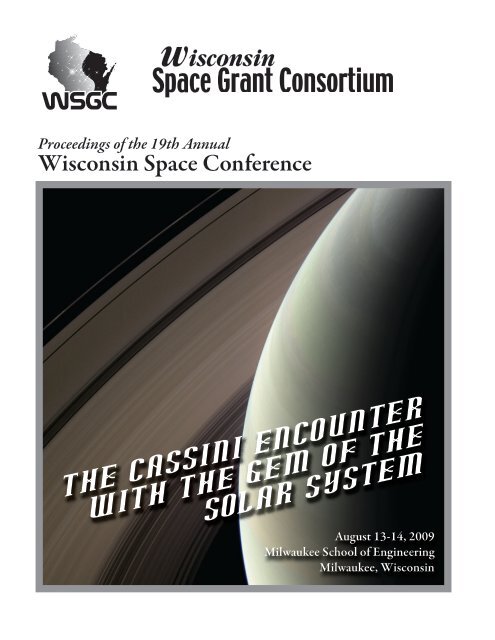
<strong>Space</strong> <strong>Grant</strong> <strong>Consortium</strong><br />
wisconsin<br />
UNIVERSITY OF WISCONSIN-GREEN BAY<br />
Proceedings <strong>of</strong> the 19th Annual<br />
<strong>Wisconsin</strong> <strong>Space</strong> Conference<br />
The Cassini Encounter<br />
with the Gem <strong>of</strong> the<br />
Solar System<br />
August 13-14, 2009<br />
Milwaukee School <strong>of</strong> Engineering<br />
Milwaukee, <strong>Wisconsin</strong>
For information about the programs <strong>of</strong> the <strong>Wisconsin</strong> <strong>Space</strong> <strong>Grant</strong> <strong>Consortium</strong>,<br />
contact the Program Office or any <strong>of</strong> the following individuals:<br />
<strong>Wisconsin</strong> <strong>Space</strong> <strong>Grant</strong> <strong>Consortium</strong><br />
<strong>University</strong> <strong>of</strong> <strong>Wisconsin</strong>-<strong>Green</strong> <strong>Bay</strong><br />
2420 Nicolet Drive<br />
<strong>Green</strong> <strong>Bay</strong>, WI 54311-7001<br />
Tel: (920)465-2108; Fax: (920)465-2376<br />
www.uwgb.edu/wsgc<br />
Director<br />
R. Aileen Yingst<br />
<strong>University</strong> <strong>of</strong> <strong>Wisconsin</strong>-<strong>Green</strong> <strong>Bay</strong><br />
(920)465-2327; yingsta@uwgb.edu<br />
Program Manager/Associate Director for Outreach<br />
Sharon D. Brandt<br />
<strong>University</strong> <strong>of</strong> <strong>Wisconsin</strong>-<strong>Green</strong> <strong>Bay</strong><br />
(920)465-2941; brandts@uwgb.edu<br />
Chair, WSGC Advisory Council and Institutional Representative<br />
Karen Valley<br />
<strong>Wisconsin</strong> Department <strong>of</strong> Transportation<br />
(608)266-8166; karen.valley@dot.state.wi.us<br />
WSGC Associate Director for Scholarships/Fellowships<br />
Steven Dutch<br />
<strong>University</strong> <strong>of</strong> <strong>Wisconsin</strong>-<strong>Green</strong> <strong>Bay</strong><br />
(920)465-2246; dutchs@uwgb.edu<br />
WSGC Associate Director for Student Satellite Programs<br />
William Farrow<br />
Milwaukee School <strong>of</strong> Engineering<br />
(414)277-2241; farroww@msoe.edu<br />
WSGC Associate Director for Research Infrastructure<br />
Gubbi R. Sudhakaran<br />
<strong>University</strong> <strong>of</strong> <strong>Wisconsin</strong>-La Crosse<br />
(608)785-8431; sudhakar.gubb@uwlax.edu<br />
WSGC Associate Director for Higher Education<br />
John Borg<br />
Marquette <strong>University</strong><br />
(414)288-7519; john.borg@marquette.edu<br />
WSGC Associate Director for Special Initiatives<br />
Thomas Bray<br />
Milwaukee School <strong>of</strong> Engineering<br />
(414)277-7416; brayt@msoe.edu<br />
WSGC Associate Director for Industry Program<br />
Eric Rice<br />
Orbital Technologies Corporation<br />
(608)827-5000; ricee@orbitec.com
THE CASSINI ENCOUNTER WITH<br />
THE GEM OF THE SOLAR SYSTEM<br />
19 th Annual <strong>Wisconsin</strong> <strong>Space</strong> Conference<br />
August 13-14, 2009<br />
Host: Milwaukee School <strong>of</strong> Engineering<br />
Milwaukee, <strong>Wisconsin</strong><br />
Edited by: R. Aileen Yingst, Director, <strong>Wisconsin</strong> <strong>Space</strong> <strong>Grant</strong> <strong>Consortium</strong><br />
Sharon D. Brandt, Program Manager, <strong>Wisconsin</strong> <strong>Space</strong> <strong>Grant</strong> <strong>Consortium</strong><br />
Martin Rudd, Assistant Pr<strong>of</strong>essor <strong>of</strong> Chemistry, UW-Fox Valley<br />
Nadejda Kaltcheva, Department <strong>of</strong> Physics & Astronomy, UW-Oshkosh<br />
Cover by: Jonathan Carlson, Student Assistant, <strong>Wisconsin</strong> <strong>Space</strong> <strong>Grant</strong> <strong>Consortium</strong><br />
Layout by: Sue Weiler, Office Coordinator, <strong>Wisconsin</strong> <strong>Space</strong> <strong>Grant</strong> <strong>Consortium</strong><br />
Published by: <strong>Wisconsin</strong> <strong>Space</strong> <strong>Grant</strong> <strong>Consortium</strong><br />
<strong>University</strong> <strong>of</strong> <strong>Wisconsin</strong>-<strong>Green</strong> <strong>Bay</strong>
��������������������������������������������������<br />
���������������������������������<br />
������������������������������������<br />
���������������������<br />
�<br />
������������5�������������<br />
�<br />
������������<br />
�<br />
���
Th he proceedinngs<br />
<strong>of</strong> our 199th<br />
Annual W<strong>Wisconsin</strong><br />
S<strong>Space</strong><br />
Confeerence<br />
comess<br />
in a<br />
mo omentous yeear.<br />
In 20099<br />
we celebrated<br />
the moost<br />
amazing, , most increedible<br />
thi ing that humman<br />
beings hhave<br />
ever doone<br />
— 40 yeears<br />
ago hummans<br />
for thee<br />
first<br />
tim me broke thee<br />
gravitationnal<br />
pull <strong>of</strong> thheir<br />
own plannet<br />
and livedd<br />
on anotherr<br />
one.<br />
Th his year hhas<br />
seen wwonderful,<br />
meaningful, , and sommetimes<br />
excciting<br />
celebbrations<br />
<strong>of</strong> th his event! UUnfortunatelyy,<br />
at the samme<br />
time, we aalso<br />
were suubjected<br />
thiss<br />
year<br />
to rerruns<br />
and new w productioons<br />
<strong>of</strong> slicklyy-produced<br />
television sppecials<br />
"sugggesting"<br />
thaat<br />
the<br />
entiree<br />
Moon land ding was a hooax.<br />
We live in n a time whhere<br />
technoloogy<br />
has madde<br />
it easier thhan<br />
ever to be fooled — and<br />
paraddoxically,<br />
wh here less andd<br />
less <strong>of</strong> a prremium<br />
seemms<br />
to be put on the criticcal<br />
thinking skills<br />
that wwould<br />
best protect p us fr from being ffooled.<br />
As eeducators<br />
(thhose<br />
<strong>of</strong> us wwho<br />
are) wee<br />
talk<br />
aboutt<br />
the importa ance <strong>of</strong> Scieence,<br />
Technoology,<br />
Enginneering<br />
and Mathematiccs<br />
(STEM) ffields.<br />
As wwe<br />
all know, however, leearning<br />
youur<br />
multiplicaation<br />
tables sso<br />
you can ppass<br />
a test iis<br />
not<br />
why STEM is so o important. . No, it's beecause<br />
to truuly<br />
be able to understand<br />
the ruless<br />
that<br />
underrlie<br />
the work kings <strong>of</strong> the universe — that is, phyysics,<br />
chemistry,<br />
mathemmatics,<br />
and sso<br />
on<br />
— yoou<br />
must have e critical thinnking<br />
skills. You must bbe<br />
able to appproach<br />
a prooblem<br />
from mmany<br />
anglees,<br />
embrace e multiple, sometimes conflicting hypothesess,<br />
apply creative<br />
soluttions,<br />
perseevere<br />
throug gh dead endss<br />
and failed experimentts<br />
and your own fatiguee<br />
and frustraation,<br />
and mmost<br />
importa antly, to let tthe<br />
universe teach you, rrather<br />
than trrying<br />
to molld<br />
the univerrse<br />
to<br />
what you want it t to be. Youu<br />
must not oonly<br />
be objecctive,<br />
but bee<br />
willing to be convinceed<br />
by<br />
superrior<br />
evidence e, especiallyy<br />
when that eevidence<br />
poinnts<br />
in a direcction<br />
you doon't<br />
want to ggo.<br />
This is why<br />
STEM fiields<br />
are releevant<br />
to all ccitizens,<br />
andd<br />
why spacee<br />
fields especcially<br />
are reelevant.<br />
Spac ce and aerosspace<br />
represeent<br />
the very edge <strong>of</strong> the envelope, annd<br />
thus the ffields<br />
where<br />
these critic cal thinking skills are mmost<br />
essentiall.<br />
This is whhy<br />
the work published heere<br />
is<br />
relevant<br />
to Wisco onsin and thhe<br />
country — because byy<br />
the very nature<br />
<strong>of</strong> whaat<br />
we are strriving<br />
for inn<br />
aerospace pursuits, p thee<br />
very best iss<br />
demanded <strong>of</strong> us. We cannot<br />
be lazzy<br />
in our thinnking<br />
or ouur<br />
work; we cannot c settlee,<br />
we cannot "make do." We must exxcel.<br />
Acknnowledgeme<br />
ents<br />
I have bee en privilegedd<br />
to review the work puublished<br />
heree,<br />
where I seee<br />
that excellence<br />
manifested.<br />
I'm grateful g to eeach<br />
person who made the 19th AAnnual<br />
Confe ference and these<br />
Proceeedings<br />
poss sible. The W<strong>Wisconsin</strong><br />
Sppace<br />
<strong>Grant</strong> C<strong>Consortium</strong><br />
especially eextends<br />
thannks<br />
to<br />
our hhost,<br />
the Mil lwaukee Schhool<br />
<strong>of</strong> Enginneering,<br />
andd<br />
WSGC Exxecutive<br />
Commmittee<br />
memmbers<br />
Tom Bray, Will liam Farroww,<br />
and especcially<br />
Loretta<br />
Krenitskyy<br />
for all thheir<br />
assistancce<br />
in<br />
runniing<br />
a beautif ful conferennce.<br />
We alsoo<br />
thank Dr. Ellis Minerr,<br />
who serveed<br />
as the Science<br />
Manaager<br />
for the NASA N Cassini-Huygenss<br />
Saturn Orbbiter<br />
and Titaan<br />
Probe for 12 years (ammong<br />
his mmany<br />
accolad des) for giviing<br />
keynote presentationns:<br />
The Casssini<br />
Encountter<br />
with the Gem<br />
<strong>of</strong> thee<br />
Solar System<br />
I & II. Dr. Minerr<br />
spoke to mmembers<br />
<strong>of</strong>f<br />
the 1997 W<strong>Wisconsin</strong><br />
S<strong>Space</strong><br />
Confference<br />
at MS SOE on the Cassini Mission<br />
before llaunch<br />
and tthis<br />
brought us full-circle.<br />
Our ssession<br />
mod derators are all volunteeers<br />
and we aare<br />
grateful for their geenerous<br />
efforrts<br />
in<br />
ensurring<br />
our ses ssions run ssmoothly.<br />
Finally,<br />
as aalways,<br />
we wwould<br />
like to thank alll<br />
the<br />
scienntists,<br />
engine eers, studentss,<br />
educators and others, wwho<br />
contribuuted<br />
papers to this volumme.<br />
Forwward!<br />
Pr reface<br />
R. Aiileen<br />
Yingst,<br />
Ph.D.<br />
Direcctor<br />
iii
Student Programs<br />
<strong>Wisconsin</strong> <strong>Space</strong> <strong>Grant</strong> <strong>Consortium</strong><br />
• Undergraduate Scholarship<br />
• Undergraduate Research<br />
• Graduate Fellowship<br />
• Dr. Laurel Salton Clark Memorial Graduate Fellowship<br />
• <strong>University</strong> Sounding Rocket Team Competition<br />
• Student High-Altitude Balloon Launch<br />
• Student High-Altitude Balloon Payload<br />
• Student High-Altitude Balloon Instrument Development<br />
• Industry Member Internships<br />
• NASA ESMD Internships<br />
• NASA Academy Leadership Internships<br />
• NASA Centers/JPL Internships<br />
• NASA Reduced/Gravity Team Launches<br />
• Relevant Student Travel<br />
(see detailed descriptions on next page)<br />
Research<br />
The Research Infrastructure Program provides<br />
Research Seed <strong>Grant</strong> Awards to faculty and staff from<br />
WSGC Member and Affi liate Member colleges and<br />
universities to support individuals interested in starting<br />
or enhancing space- or aerospace-related research<br />
program(s).<br />
Higher Education<br />
The Higher Education Incentives Program is a seedgrant<br />
program inviting proposals for innovative,<br />
value-added, higher education teaching/training<br />
projects related to space science, space engineering,<br />
and other space- or aerospace-related disciplines. The<br />
Student Satellite Program including Balloon and Rocket<br />
programs is also administered under this program.<br />
Industry Program<br />
The WSGC Industry Program is designed to meet the<br />
needs <strong>of</strong> <strong>Wisconsin</strong> Industry member institutions in<br />
multiple ways including:<br />
1) the Industry Member Internships (listed under<br />
students above),<br />
2) the Industry/Academic Research Seed Program<br />
designed to provide funding and open an avenue for<br />
member academia and industry researchers to work<br />
together on a space-related project, and<br />
3) the Industrial Education and Training Program<br />
designed to provide funding for industry staff members<br />
to keep up-to-date in NASA-relevant fi elds.<br />
Programs for 2009<br />
v<br />
Aerospace Outreach Program<br />
The Aerospace Outreach Program provides grant<br />
monies to promote outreach programs and projects that<br />
disseminate aerospace and space-related information to<br />
the general public, and support the development and<br />
implementation <strong>of</strong> aerospace and space-related curricula<br />
in <strong>Wisconsin</strong> classrooms. In addition, this program<br />
supports NASA-trained educators in teacher training<br />
programs.<br />
Special Initiatives<br />
The Special Initiatives Program is designed to provide<br />
planning grants and program supplement grants<br />
for ongoing or new programs which have space or<br />
aerospace content and are intended to encourage,<br />
attract, and retain under-represented groups, especially<br />
women, minorities and the developmentally challenged,<br />
in careers in space- or aerospace-related fields.<br />
<strong>Wisconsin</strong> <strong>Space</strong> Conference<br />
The <strong>Wisconsin</strong> <strong>Space</strong> Conference is an annual conference<br />
featuring presentations <strong>of</strong> students, faculty, K-12<br />
educators and others who have received grants from<br />
WSGC over the past year. The Conference allows all to<br />
share their work with others interested in <strong>Space</strong>. It also<br />
includes keynote addresses, and the announcement <strong>of</strong><br />
award recipients for the next year.<br />
Regional Consortia<br />
WSGC is a founding member <strong>of</strong> the Great Midwest<br />
Regional <strong>Space</strong> <strong>Grant</strong> Consortia. The Consortia consists<br />
<strong>of</strong> eight members, all <strong>Space</strong> <strong>Grant</strong>s from Midwest and<br />
Great Lakes States.<br />
Communications<br />
WSGC web site www.uwgb.edu/wsgc provides<br />
information about WSGC, its members and programs,<br />
and links to NASA and other sites.<br />
Contact Us<br />
<strong>Wisconsin</strong> <strong>Space</strong> <strong>Grant</strong> <strong>Consortium</strong><br />
<strong>University</strong> <strong>of</strong> <strong>Wisconsin</strong>–<strong>Green</strong> <strong>Bay</strong><br />
2420 Nicolet Drive, ES 301<br />
<strong>Green</strong> <strong>Bay</strong>, <strong>Wisconsin</strong> 54311-7001<br />
Phone: (920) 465-2108<br />
Fax: (920) 465-2376<br />
E-mail: wsgc@uwgb.edu<br />
Website: www.uwgb.edu/wsgc
<strong>Wisconsin</strong> <strong>Space</strong> <strong>Grant</strong> <strong>Consortium</strong><br />
Undergraduate Scholarship Program<br />
Supports outstanding undergraduate students pursuing<br />
aerospace, space science, or other space-related studies<br />
or research.<br />
Undergraduate Research Awards<br />
Supports qualifi ed students to create and implement<br />
a small research study <strong>of</strong> their own design during the<br />
summer or academic year that is directly related to<br />
their interests and career objectives in space science,<br />
aerospace, or space-related studies.<br />
Graduate Fellowships<br />
Support outstanding graduate students pursuing<br />
aerospace, space science, or other interdisciplinary<br />
space-related graduate research.<br />
Dr. Laurel Salton Clark Memorial<br />
Graduate Fellowship<br />
In honor <strong>of</strong> Dr. Clark, Columbia <strong>Space</strong> Shuttle<br />
astronaut and resident <strong>of</strong> <strong>Wisconsin</strong>, this award<br />
supports a graduate student pursuing studies in the<br />
fi elds <strong>of</strong> environmental or life sciences, whose research<br />
has an aerospace component.<br />
<strong>University</strong> Sounding Rocket Team<br />
Competition<br />
Provides an opportunity and funding for student teams<br />
to design and fl y a rocket that excels at a specifi c goal<br />
that is changed annually.<br />
High School Sounding Rocket Team<br />
Competition<br />
For high school students. This program is in its initial<br />
stages. It mimics the university competition.<br />
Student High-Altitude Balloon<br />
Instrument Development<br />
Students participate in this instrument development<br />
program through engineering or science teams.<br />
Working models created by the students will be fl own<br />
on high-altitude balloons.<br />
Student Programs for 2009<br />
vi<br />
Student High-Altitude Balloon Payload/<br />
Launch Program<br />
The Elijah Project is a high-altitude balloon program in<br />
which science and engineering students work in integrated<br />
science and engineering teams, to design, construct,<br />
launch, recover and analyze data from a high-altitude<br />
balloon payload. These balloons travel up to 100,000 ft.,<br />
considered “the edge <strong>of</strong> space.” Selected students will<br />
join either a launch team or a payload design team.<br />
Industry Member Internships<br />
Supports student internships in space science or<br />
engineering for the summer or academic year at WSGC<br />
Industry members co-sponsored by WSGC and Industry<br />
partners.<br />
NASA ESMD Internships<br />
Supports student internships at NASA centers or WSGC<br />
industry members that tie into NASA’s Exploration<br />
Systems Mission Directorates.<br />
NASA Academy Leadership Internships<br />
This summer internship program at NASA Centers<br />
promotes leadership internships for college juniors, seniors<br />
and fi rst-year graduate students and is co-sponsored by<br />
participating state <strong>Space</strong> <strong>Grant</strong> Consortia.<br />
NASA Centers/JPL Internships<br />
Supports WSGC students for research internships at<br />
NASA Centers or JPL.<br />
NASA Reduced Gravity Program<br />
Operated by the NASA Johnson <strong>Space</strong> Center, this<br />
program provides the unique “weightless” environment<br />
<strong>of</strong> space fl ight for test and training purposes. WSGC<br />
student teams submit reduced gravity experiments to<br />
NASA and, if selected, get to perform their experiments<br />
during a weightless environment fl ight with the support<br />
<strong>of</strong> WSGC.<br />
Relevant Student Travel<br />
Supports student travel to present their WSGC-funded<br />
research.
Preface<br />
19th Annual Conference<br />
TABLE OF CONTENTS<br />
Part 1: Student Satellite Program: High Altitude Balloon<br />
Balloon Launch Team:<br />
Eric Deering, Milwaukee School <strong>of</strong> Engineering<br />
Brian Nguyen, Milwaukee School <strong>of</strong> Engineering<br />
Nathan Sward, Milwaukee School <strong>of</strong> Engineering<br />
Balloon Payload Team:<br />
Antonio Castillo, <strong>University</strong> <strong>of</strong> <strong>Wisconsin</strong>-Madison<br />
Brittany Hauser, Milwaukee School <strong>of</strong> Engineering<br />
Zachary Parsons, Milwaukee School <strong>of</strong> Engineering<br />
Chris Reichard, Milwaukee School <strong>of</strong> Engineering<br />
Victorialynn Salas, Marquette <strong>University</strong><br />
Max Witte, Milwaukee School <strong>of</strong> Engineering<br />
Part 2: Student Satellite Program: Rocket Design Competition<br />
1 st Place – Non Engineering<br />
Schmitt Triggers<br />
Brad Hartl, <strong>University</strong> <strong>of</strong> <strong>Wisconsin</strong>-La Crosse<br />
Jacob Wardon, <strong>University</strong> <strong>of</strong> <strong>Wisconsin</strong>-La Crosse<br />
Steven Welter, Western Technical College<br />
Mark Witte, <strong>University</strong> <strong>of</strong> <strong>Wisconsin</strong>-La Crosse<br />
1 st Place – Engineering<br />
Team Narwhal, Milwaukee School <strong>of</strong> Engineering<br />
Neal Bitter, Team Leader<br />
Adam Harden<br />
Chelsey Jelinski<br />
2 nd Place - Engineering<br />
Team Drew and Crew - Milwaukee School <strong>of</strong> Engineering<br />
Drew Falkenburg, Team Leader<br />
Wes Larrabee<br />
Caleb Varner<br />
3rd Place - Engineering<br />
Rocky Mountain Miners - Milwaukee School <strong>of</strong> Engineering<br />
Brian Mortensen, Team Leader<br />
Ryan May<br />
Jon Neujahr<br />
vii
Part 3: NASA Reduced Gravity Programs<br />
Part 4: Engineering<br />
Repose Angles <strong>of</strong> Lunar Mare Simulants in Microgravity, Isa Fritz, Erin Martin,<br />
Samantha Kreppel, Brad Frye, and Caitlin Pennington, Undergraduate Students,<br />
Carthage College<br />
Dynamics Characterization <strong>of</strong> the Electron Beam Freeform Fabrication System<br />
Matthew Kallerud, Undergraduate Student, Milwaukee School <strong>of</strong> Engineering<br />
Analysis <strong>of</strong> Circulation Properties in Wake Vortices, Vanessa Peterson,<br />
Undergraduate Student, <strong>University</strong> <strong>of</strong> <strong>Wisconsin</strong>-Madison<br />
Validation <strong>of</strong> Novel Rigid Body Frictional Contact Algorithms using Tracked<br />
Vehicle, Simulation: A Stepping Stone for Billion Body Dynamics, Justin<br />
Madsen, Graduate Student, <strong>University</strong> <strong>of</strong> <strong>Wisconsin</strong>-Madison<br />
Modeling and Optimization <strong>of</strong> a Two Stage Mixed Gas Joule-Thomson<br />
Cryocooler, Harrison Skye, Graduate Student, <strong>University</strong> <strong>of</strong> <strong>Wisconsin</strong>-Madison<br />
ECLSS Vapor Compression Distillation System and Brine Processing, Cheryl<br />
Perich, Undergraduate Student, Marquette <strong>University</strong><br />
Phaeton Mast Dynamics Mechanical Systems, Adam Harden, Undergraduate<br />
Student, Milwaukee School <strong>of</strong> Engineering<br />
Risk Mitigation Study for ISIM Systems Engineering, Code 443, Aaron Olson,<br />
Undergraduate Student, <strong>University</strong> <strong>of</strong> <strong>Wisconsin</strong>-Madison<br />
Part 5: Atmospheric Science<br />
Part 6: Astronomy<br />
Is Lake Superior a Significant Source <strong>of</strong> Atmospheric Carbon Dioxide?, Val<br />
Bennington, Graduate Student, <strong>University</strong> <strong>of</strong> <strong>Wisconsin</strong>-Madison<br />
Realizing a Better Hydrostatic Response in NWP with MODIS Products, Jordan<br />
Gerth, Undergraduate Student, <strong>University</strong> <strong>of</strong> <strong>Wisconsin</strong>-Madison<br />
A Comparative Study <strong>of</strong> Type IIb Supernovae, Bradley Rentz, Cyrus Vandrevala<br />
and Michael Heim, Undergraduate Students, Marquette <strong>University</strong><br />
Gravitational Heating and Evolution <strong>of</strong> Galaxy Groups, Melania Riabokin,<br />
Undergraduate Student, <strong>University</strong> <strong>of</strong> <strong>Wisconsin</strong>-Madison<br />
viii
Part 7: Physics<br />
Understanding the Evolution <strong>of</strong> Supernova Progenitors, Cyrus Vandrevala and<br />
Bradley Rentz, Undergraduate Students, Marquette <strong>University</strong><br />
Computational Fluid Dynamical Model <strong>of</strong> a Cyclone Separator in Microgravity,<br />
Brad Frye, Undergraduate Student, Department <strong>of</strong> Physics, Carthage College<br />
Simulation <strong>of</strong> Fast Magnetic Reconnection using a Two-Fluid Model <strong>of</strong><br />
Collisionless Pair Plasma without Anomalous Resistivity, E. Alec Johnson,<br />
Graduate Student, Department <strong>of</strong> Mathematics, <strong>University</strong> <strong>of</strong> <strong>Wisconsin</strong>-Madison<br />
Part 8: Biological Science<br />
Part 9: Chemistry<br />
Reflection and Refraction <strong>of</strong> Vortex Rings, Kerry Kuehn, Associate Pr<strong>of</strong>essor,<br />
Department <strong>of</strong> Physical Sciences, <strong>Wisconsin</strong> Lutheran College<br />
Understanding Risk Determinants <strong>of</strong> Chagas Disease in Peri-urban Peru,<br />
Megan Christenson, Graduate Student, <strong>University</strong> <strong>of</strong> <strong>Wisconsin</strong>-Madison<br />
Astronaut Advanced Life Support: Engineering Extra Terrestrial Extremophile<br />
Plants, Dan Hawk, Undergraduate Student, College <strong>of</strong> Menominee Nation<br />
Toxic Offgassing Analysis at Marshall <strong>Space</strong> Flight Center, Kenion Blakeman,<br />
Undergraduate Student, Department <strong>of</strong> Chemistry, Carthage College<br />
Preparation and Characterization <strong>of</strong> Platinized Electrodes for Use in Oxygen<br />
Extraction from Lunar Regolith, Nathan Wong, Undergraduate Student,<br />
<strong>University</strong> <strong>of</strong> <strong>Wisconsin</strong>-Madison<br />
New Initiatives in the Project on Fossilization via Silicification, Vera Kolb,<br />
Pr<strong>of</strong>essor, Department <strong>of</strong> Chemistry, <strong>University</strong> <strong>of</strong> <strong>Wisconsin</strong>-Parkside and<br />
Patrick Liesch, Department <strong>of</strong> Entomology, <strong>University</strong> <strong>of</strong> <strong>Wisconsin</strong>-Madison<br />
Part 10: Education and Public Outreach<br />
Combining Writing Across the Curriculum Strategies in Community-Based<br />
Programs to Teach Core Scientific Concepts, James Kramer, Executive Director,<br />
Simpson Street Free Press<br />
Educators’ Aerospace Workshop for the 21 st Century, Jake W. Blake, 8 th Grade<br />
Science Teacher, Brookwood Middle School<br />
Teaching the Teachers, Coggin Heeringa, Director, Crossroads at Big Creek<br />
Environmental Learning Preserve<br />
ix
EAA Women Soar – You Soar, Lee Siudzinski, Manager, Education<br />
Relationships, Experimental Aircraft Association (EAA)<br />
EAA <strong>Space</strong> Week 2008, Lee Siudzinski, Manager, Education Relationships,<br />
Experimental Aircraft Association (EAA) and Chrissy Paape, Vice President,<br />
<strong>Space</strong> Explorers, Inc.<br />
<strong>Space</strong> Travel Simplified – Part 1, Bradley J. Staats, President, <strong>Space</strong>flight<br />
Fundamentals, LLC<br />
Expanding GIS Across the Curriculum, Jennifer Johanson, Associate Pr<strong>of</strong>essor,<br />
Physical Science Department, Alverno College<br />
Astronautics Course, Harald Schenk, Associate Lecturer, Physics/Astronomy<br />
Department, <strong>University</strong> <strong>of</strong> <strong>Wisconsin</strong>-Sheboygan<br />
New Directions in Astrobiology Education, Vera Kolb, Pr<strong>of</strong>essor, Department <strong>of</strong><br />
Chemistry, <strong>University</strong> <strong>of</strong> <strong>Wisconsin</strong>-Parkside<br />
Providing High School Students with Earth Imaging Tools, Thomas Jeffery,<br />
Assistant Pr<strong>of</strong>essor, Geography and Geology Department, <strong>University</strong> <strong>of</strong><br />
<strong>Wisconsin</strong>-Whitewater<br />
Appendix A: 19 th Annual Conference 2009 Program<br />
x
19th Annual Conference<br />
Part One<br />
Student Satellite Program<br />
High Altitude Balloon
Elijah High Altitude Balloon Project Launch Team<br />
Eric Deering from Milwaukee School <strong>of</strong> Engineering; Brian Nguyen from Milwaukee School <strong>of</strong><br />
Engineering; and Nathan Sward from Milwaukee School <strong>of</strong> Engineering.<br />
Please note: Due to the deadline for this report, it will primarily be about the first launch <strong>of</strong> 2009. The<br />
responsibilities <strong>of</strong> the Launch Team extend through the summer and the following academic year, and<br />
accommodate both the Payload Team and the Instrumentation Team. Multiple future launches are<br />
planned, therefore, which are not covered in this report.<br />
Members and Roles<br />
Because the Launch Team has only three members this year, each member is involved with all aspects <strong>of</strong><br />
the project. However, Eric Deering served as the primary liaison in communications with WSGC and<br />
StratoStar. All members bring some experience to the table, since Brian Nguyen and Nathan Sward<br />
were on the Payload Team last year, and Eric Deering was on the HALO II project.<br />
Equipment<br />
Overview<br />
The 2009 Launch Team is again using the StratoSat complete flight package, by StratoStar Systems. This<br />
system was first used by the 2008 team and was found to be an excellent tool. The system contains<br />
everything necessary to plan, launch, and remotely track the payload. The following components are<br />
included:<br />
• Command pod with GPS and data<br />
transmitter<br />
• Three payload pods<br />
• Two 900 Mhz Modules and antennae<br />
• StratoStar s<strong>of</strong>tware, which interacts<br />
with Micros<strong>of</strong>t MapPoint<br />
• Battery chargers for the pods<br />
• Parachute<br />
• Cables and tethering<br />
Figure 1: StratoSat System<br />
In addition to the StratoStar package, the launch team acquired high altitude weather balloons, helium,<br />
and the payload to be carried, which was supplied by the payload team.<br />
Balloons<br />
The Elijah launch team began the season using a 1200 gram balloon that was left over from last season.<br />
After witnessing the performance <strong>of</strong> the first balloon and after talking with the company who sells the<br />
balloons (Kaymont), the decision was made to purchase two more 1200 gram balloons for future flights.<br />
1
From some <strong>of</strong> the information Kaymont had on their website regarding balloon performance we were<br />
able to get a better idea <strong>of</strong> how our balloons should be performing. The 1200 gram balloons we<br />
purchased had an average ascent rate <strong>of</strong> 1050 feet per minute with an average bursting altitude <strong>of</strong> a<br />
little over 30 kilometers. This now gave us some ground statistics which would allow us to better predict<br />
landing locations for future launches.<br />
Command and Payload Pods<br />
The StratoSat system comes with one command pod and three payload pods. The command pod is<br />
responsible for flight data acquisition such as position, altitude, speed, and heading while the payload<br />
pods can be set up with other sensors to collect data such as temperature and pressure. The payload<br />
pods can communicate wirelessly with the command pod which sends all <strong>of</strong> the information gathered by<br />
both the command pod and the payload pod back to the tracking s<strong>of</strong>tware. Once tracking is complete<br />
the data can be simply exported into an excel file and analyzed even without the recovery <strong>of</strong> the system.<br />
Equipment Testing<br />
Since the tracking <strong>of</strong> our balloons was to be done with StartoStar Systems StratoSat setup, we began by<br />
installing Micros<strong>of</strong>t MapPoint and the StratoStar s<strong>of</strong>tware. The new StratoStar s<strong>of</strong>tware conveniently<br />
interfaced with Micros<strong>of</strong>t MapPoint which allowed for easy geographical location <strong>of</strong> the balloon. Before<br />
our first launch we took all <strong>of</strong> the StratoSat equipment outside to verify it was working properly. After<br />
overcoming a few obstacles with the USB to serial converters, we were able to locate the command pod<br />
on our computers. After tracking one <strong>of</strong> our team members driving around Milwaukee we concluded<br />
that the equipment was working properly.<br />
Our team quickly noticed that the command pods transmitter needed to be directionally positioned to<br />
the antenna receiver. For example, when the transmitter was pointed away from the antenna, the GPS<br />
transmitter on the command pod could not communicate with the receiver. While this remains an issue<br />
once the balloon is on the ground, this problem is diminished when the balloon is high above the GPS<br />
receiver.<br />
High Altitude Launch Opportunity (HALO) II<br />
The <strong>Wisconsin</strong> <strong>Space</strong> <strong>Grant</strong> Balloon Launch Team began its annual duties in the 2009-2010 season by<br />
participating in the High Altitude Launch Opportunity (HALO II) this spring. The HALO II project consisted<br />
<strong>of</strong> the simultaneous launching <strong>of</strong> 15 high altitude balloons from 15 universities in 9 different states. The<br />
purpose <strong>of</strong> the HALO II launch was to set up a high altitude communications network along with<br />
collecting temperature, humidity, pressure, altitude, CO2, rate, and radiation data. By having each<br />
payload transmit a radio frequency, the different balloons could link together through the radio<br />
transmissions and share data. Taylor <strong>University</strong> in Indiana served as the mission control for the project<br />
and through the communication network created, could receive data in real time. This eliminated the<br />
need for a sometimes unsuccessful recovery <strong>of</strong> the balloon.<br />
2
Our experience with the HALO II launch<br />
went well and was a good starting point<br />
for the rest <strong>of</strong> the season. We were able<br />
to experience some <strong>of</strong> the basic<br />
procedures such as caring for and filling<br />
the balloon along with practicing with the<br />
s<strong>of</strong>tware and the payload unit that was<br />
sent to us from StratoStar. While the<br />
procedures <strong>of</strong> the launch and actually<br />
launching the balloon went well, tracking<br />
and recovering the balloon was a different<br />
story. Up to about half way through the<br />
balloons flight, the tracking s<strong>of</strong>tware was<br />
working well and was transmitting GPS<br />
points back to our s<strong>of</strong>tware. However,<br />
shortly after the balloon reached Figure 2: HALO II Network Coverage<br />
approximately 100,000ft we stopped<br />
receiving GPS and data packages. After driving around for about four hours trying to pick up a signal on<br />
the payload, our team was forced to abort the recovery mission.<br />
A few weeks ago our team contacted Jason Krueger from StratoStar to try and figure out the reason for<br />
the GPS failure. His conclusion was that the payloads aerodynamic design caused it to twist and turn,<br />
eventually becoming tangled in the cord, causing the antenna to break <strong>of</strong>f. We were not the only team<br />
to have trouble with tracking and data transmission so hopefully these problems will be corrected for<br />
the next team that decides to partake in the continuing HALO project.<br />
For more information on the HALO II launch you can go to the following website<br />
http://www.nearspacenetwork.com/group/halo2project<br />
Launch Planning<br />
Balloon Choice<br />
As stated above our team chose to use 1200 gram balloons for our launches. 1200 gram balloons are<br />
relatively small so they allow us to maximize our use <strong>of</strong> helium while still providing ample lift for any<br />
payload the team may choose to send up. 1200 gram balloons also have similar maximum height and<br />
ascent rate characteristics when compared with larger balloons.<br />
Location Choice<br />
An optimal location for a launch is dependent upon 1) the ideal location <strong>of</strong> landing, 2) weather<br />
conditions, and 3) risk factors in the area. The ideal location <strong>of</strong> a landing would be in a rural location,<br />
away from power lines and heavy traffic. Further, it would be someplace that is not heavily wooded,<br />
since this makes retrieval difficult. The location for which we aimed for our first launch was near<br />
Monroe, <strong>Wisconsin</strong>. This is a rural, sparsely populated area, with less trees and hills than Western<br />
<strong>Wisconsin</strong>.<br />
3
Prediction S<strong>of</strong>tware<br />
To be able to accurately predict where a high altitude balloon will land is next to impossible unless you<br />
are able to consider all <strong>of</strong> the variables that come into play. Fortunately, flight prediction s<strong>of</strong>tware<br />
based online at (www.nearspaceventures.com) is able to consider all <strong>of</strong> these variables and put them to<br />
use. This s<strong>of</strong>tware takes into account the weather predictions for the area in question and plots take<br />
<strong>of</strong>f, landing, and balloon burst points on a map.<br />
In days leading up to the launch, flight prediction s<strong>of</strong>tware was used to predict the course <strong>of</strong> the flight<br />
using weather forecast details from the closest weather station and details about ascent and descent<br />
rate which we obtained from the balloon manufacturer. This tool was first used to predict the flight<br />
path from Boscobel, WI. The s<strong>of</strong>tware predicted that the payload would land near Dubuque, Iowa,<br />
which was unacceptable. Mt. Horeb, WI was finally decided on as the most convenient site that would<br />
result in a landing location around Monroe, WI.<br />
For the second launch the same prediction s<strong>of</strong>tware from (www.nearspaceventures.com) was used to<br />
again try and find an optimal landing zone as discussed above. Below is a figure showing the results <strong>of</strong><br />
the prediction for the second launch.<br />
Figure 3: Flight Prediction for Launch 2<br />
Launch Day<br />
Launch<br />
On Saturday July 18 th , the launch team and 4 members <strong>of</strong> the payload team headed to Mt. Horeb to<br />
execute the first launch <strong>of</strong> the 2009-2010 season. The first task for making our first launch successful<br />
was finding a safe place to launch the balloon. By using the satellite view on Google maps we were able<br />
to find a nearby football field. The launch site worked well due to the fact that it had no trees or power<br />
lines in the immediate area and the site was elevated relative to the surroundings.<br />
After finding the site we brought out all <strong>of</strong> our gear and laid out everything we would need on the grass.<br />
A tarp was laid on the ground so the balloon could be filled without causing any damage to it. Rubber<br />
gloves were worn by the launch team members when handling the balloon to avoid getting skin oil on<br />
the balloon which can hamper the balloons expansion at high altitudes. The balloon was then filled<br />
4
which had been a problem in the past due to a check valve in the connection fitting to the helium tank.<br />
After unsuccessfully looking for a new tank fitting without a check valve, the decision was made to<br />
simply drill out the check valve to provide better air flow. This decision proved to be a success as the fill<br />
time <strong>of</strong> the balloon went from about 2 hours to 15 minutes. While the fitting now doesn’t have a check<br />
valve it is still safe since the flow <strong>of</strong> helium can be regulated by the tanks<br />
valve.<br />
At approximately 11:00AM the balloon and the payloads underwent a final<br />
check along with turning the GPS system on and checking to see how it was<br />
performing. A few minutes later the balloon was released and instantly we<br />
knew something wasn’t right. The balloon slowly began ascending and then<br />
started descending. The members present rushed to grab the balloon and it<br />
was brought back to the launch pad. An oversight had been made while<br />
reading the scale which measured the amount <strong>of</strong> lift the balloon was<br />
providing. Since the wind was blowing the balloon sideways while the lift<br />
was being measured, the wind added on to the amount <strong>of</strong> lift significantly.<br />
After holding the balloon steady we were able to get the lift up to around<br />
6lbs, about 3/2 the weight <strong>of</strong> our payload.<br />
The balloon was released a second time, this time with much better results.<br />
The members present watch the balloon rise away and then proceeded to<br />
pick up all <strong>of</strong> the gear and<br />
begin tracking the balloon.<br />
Figure 5: GPS Generated Track <strong>of</strong> Balloon Flight<br />
Figure 4: Balloon and Payload<br />
Tracking<br />
Possibly the most fun part <strong>of</strong> being a member <strong>of</strong> the<br />
balloon launch team is tracking the balloons.<br />
Following the balloon on our laptops, our convoy <strong>of</strong><br />
three vehicles drove around back roads trying to stay<br />
close to the balloon. We had set up two laptops in<br />
separate cars, both tracking the balloon. This reduced<br />
the risk <strong>of</strong> losing the balloon due to computer<br />
problems. We tracked the balloon from Mt. Horeb,<br />
WI to just north <strong>of</strong> Monroe, WI. The StratoSat<br />
tracking system preformed well and got us to the<br />
landing point.<br />
5
Local Search<br />
While we were right under the balloon when it came down we were unable to see it. This began a long<br />
process <strong>of</strong> trying to find the balloon in a wooded area. We knew the balloon was close but we were<br />
unable to obtain a final landing point from the tracking system. Due to the directional nature <strong>of</strong> the<br />
antenna and transmitter as discussed above, it is very have to obtain tracking information once the<br />
balloon is on the ground. Once the search area was narrowed down using our GPS systems, we began<br />
to look in a limited area for the balloon. After talking with the landowner, he volunteered to help us try<br />
and find the balloon. Following about four hours <strong>of</strong> searching the woods with trucks, an ATV, and on<br />
foot, we had to call it a day. We were not able to find the unit even though the system had worked<br />
perfectly.<br />
Ideas for Future Launches<br />
The largest problem with the current system is the directional nature <strong>of</strong> the antenna and transmitter.<br />
Once the balloon is on the ground the only way to find it is to get a final landing point and then go to<br />
that point and search the area. Sometimes the final point is obtained while the balloon is still in the air,<br />
allowing the balloon to drift an unpredictable distance before landing. A solution to this came in the<br />
form <strong>of</strong> a radio tracking system that the launch team had purchased previously. The system was in need<br />
<strong>of</strong> a new tracking collar and so one was purchased and the system was tested. With an ideal range <strong>of</strong> up<br />
to seven miles the new secondary tracking system seemed ideal for short range tracking.<br />
Another idea to try and locate the payload once the balloon was on the ground came in the form <strong>of</strong> a<br />
loud beeper. This beeper made a sound similar to that <strong>of</strong> a truck back up alarm. This would allow us to<br />
audibly locate the payload from well over 100 yard away.<br />
Lastly, since we had determined the parachute had not opened in our first launch due to our high<br />
decent rate data, we wanted to find a way to more consistently have the parachute open. We<br />
determined that making the cord from the top <strong>of</strong> the parachute to the balloon slightly longer would give<br />
the parachute more time to fill with air after the balloon had popped.<br />
Second Launch<br />
Armed with our new secondary tracking system and the loud beeper we were confident we would<br />
retrieve the payload after our second launch. After running the prediction s<strong>of</strong>tware each day the<br />
previous week, Mt. Horeb was again determined as an ideal launch site. The prediction for this flight<br />
(Figure 3 ) told us the balloon would travel north east, landing in south central <strong>Wisconsin</strong>. After getting<br />
everything unpacked some weather began to roll in, threatening our ability to launch. With still an hour<br />
before the storm hit we decided to launch the balloon. This time the balloon was carrying the payload<br />
team’s experiments, a secondary radio tracking device, the StratoStar command pod, and a very loud<br />
beeper.<br />
After tracking the balloon for a little over an hour the balloon hovered over the Horicon marsh for 30<br />
minutes at an approximate altitude <strong>of</strong> 25 kilometers. While the balloon remained in the same position<br />
horizontally, it slowly climbed in altitude where it finally popped at around 30 kilometers. The balloon<br />
again began traveling northeast during its descent. Staying just ahead <strong>of</strong> the looming storm we tracked<br />
the balloon across highway 41 where it landed just east <strong>of</strong> Lomira.<br />
6
Figure 6: 3-D GPS Generated Track <strong>of</strong> Balloon Flight<br />
Using our secondary tracking device we were able to locate a general area in which we thought the<br />
balloon had landed. Heading in on foot with the radio tracking device we continued in the direction <strong>of</strong><br />
the strongest signal until we heard a noise. It was the beeper on the payload which seemed to be just<br />
beyond a patch <strong>of</strong> woods. When we arrived at the payload we were both excited to have found the<br />
system, and disappointed to see that it was stuck 60 feet up in a tree. With no means <strong>of</strong> retrieving the<br />
payload from the tree we were forced to temporarily abandon our payload.<br />
Conclusion<br />
The launch team has identified some problems with the system <strong>of</strong> launching and retrieving the balloons<br />
but has also come up with solutions to many <strong>of</strong> those problems. The solution to finding the balloon<br />
after it was on the ground came in two separate systems. The radio collar tracking system and the loud<br />
beeper that was placed on the payload for easier short range recovery. The radio tracking system led us<br />
to the payload where we were then able to hear the alarm and locate the payload in a tree. Also,<br />
adding a few feet to the tether between the balloon and the parachute solved the problem <strong>of</strong> the chute<br />
not opening.<br />
These additional systems have greatly increased the percentage <strong>of</strong> balloon recovery. While our first<br />
launch recovery was unsuccessful even with the StratoSat system performing well, our team was able to<br />
come up with secondary systems to aid in the recovery <strong>of</strong> the balloons. With multiple launches in the<br />
team’s future, we plan to further refine the system <strong>of</strong> launching and recovering high altitude balloons to<br />
make it easier on teams in the future.<br />
7
2009 Elijah Summer Payload Team<br />
Antonio Castillo, <strong>University</strong> <strong>of</strong> <strong>Wisconsin</strong>-Madison<br />
Brittany Hauser, Milwaukee School <strong>of</strong> Engineering<br />
Zachary Parsons, Milwaukee School <strong>of</strong> Engineering<br />
Chris Reichard, Milwaukee School <strong>of</strong> Engineering<br />
Victoria Salas, Marquette <strong>University</strong><br />
Max Witte, Milwaukee School <strong>of</strong> Engineering<br />
Project Synopsis<br />
The Elijah Payload Project is an opportunity for science and engineering students to research,<br />
design, develop, and implement their own experiments. A high altitude weather balloon is<br />
launched into the stratosphere with the students’ designed payload attached. There are no limits<br />
other than weight as to what can be included in this payload; the students are encouraged to<br />
develop their own ideas over the course <strong>of</strong> the 10-week program. Through weekly meetings and<br />
brainstorming sessions, four separate experiments were designed and constructed. The first<br />
payload was lost and the second has not been launched as <strong>of</strong> the writing <strong>of</strong> this paper, but what<br />
follows is a detailed summary <strong>of</strong> the projects <strong>of</strong> the 2009 Elijah Payload Team.<br />
Seed Germination<br />
Abstract The purpose <strong>of</strong> the watermelon seed experiment is to determine if the near space<br />
environment at 100,000 feet has an effect on the seeds. This was tested by first growing the seeds<br />
and then comparing the growth <strong>of</strong> the experimental seeds to the growth <strong>of</strong> the control seeds.<br />
Background Everything on earth is exposed to small amounts <strong>of</strong> natural radiation (Health<br />
Physics Society, 2001). Exposing seeds to higher amounts <strong>of</strong> radiation can cause inhibited<br />
sprouting, slow seedling growth, reduced plant fertility, and chromosome alterations.<br />
Watermelon seeds were chosen because they have a fast germination <strong>of</strong> three to seven days and<br />
do not require a special environment for growth.<br />
Methodology Four bottles with approximately 15 seeds in each bottle were created. Two bottles<br />
with seeds were sent up with the balloon; one insulated and the other not insulated. The other<br />
two bottles were used as controls; one staying at MSOE and the other traveling with the<br />
experimental seeds until the launch. Since the payload was not recovered, the seeds were tested<br />
in the lab with a bell jar and dry ice.<br />
The three packs <strong>of</strong> seeds purchased are Sugar Baby Watermelon Seeds, packed in 4g packages<br />
by the Livingston Seed Co. All three packages <strong>of</strong> seeds were labeled 2009 Run B, sell by 10/09.<br />
The seeds were planted in a 72 cell seed insert with Stein seed starter mix. The seed tray was<br />
placed in an 11” x 22” base tray and covered with a two inch tall humidity dome. The seed tray<br />
was then placed on a Hydr<strong>of</strong>arm heated germination station that uses 120V and 17W. Two 13W<br />
Ott lights, model # OTL13BPB, were placed above the seeds to provide light and approximately<br />
three ml <strong>of</strong> distilled water has been given to each seed daily.<br />
9
Results The seeds tested in the lab were planted on 08/05/09 and have not germinated yet. A<br />
photo <strong>of</strong> the setup for planting and the reference plants can be seen in Figure 1. Control seeds<br />
were planted on 07/27/09 for reference and are growing well. Four experimental groups were<br />
tested in the lab with fifteen seeds in each new group; control seeds, seeds exposed to the dry ice<br />
for an hour, seeds exposed to the vacuum for an hour, and seeds exposed to both the dry ice and<br />
the vacuum for an hour<br />
each.<br />
Figure 1: Watermelon seed germination container<br />
Conclusion Due to the fact that we could not retrieve the payload a conclusive decision about<br />
this experiments success or failure could not be made at this time.<br />
References "Answer to Question #1280 Submitted to "Ask the Experts"." Health Physics Society<br />
Radiation Effects — Biological Effects <strong>of</strong> Radiation 18 OCT 2001 Web.10 June 2009.<br />
.<br />
C<strong>of</strong>fee Taste<br />
Abstract The c<strong>of</strong>fee experiment was based on how the atmosphere at 100,000 feet would affect<br />
the taste <strong>of</strong> the c<strong>of</strong>fee in a near space environment, with interest developing from how<br />
microgravity affects the taste <strong>of</strong> food for astronauts. Four samples <strong>of</strong> c<strong>of</strong>fee beans were prepared<br />
and the difference in taste were compared with the sample being subjected to extreme cold<br />
having the best taste and the control sample having the worst taste.<br />
Background Motivation for this experiment developed with the team members interest in how<br />
different types <strong>of</strong> foods and beverages taste differently in space. This was later narrowed down to<br />
how the flavor <strong>of</strong> c<strong>of</strong>fee will be affected once placed into near space conditions. The genuine<br />
10
taste <strong>of</strong> c<strong>of</strong>fee and the fresh aroma are commonplace here on earth but becomes a luxury up in<br />
space for those serving on a space mission or living aboard the international space station. Food<br />
as well as c<strong>of</strong>fee is known to taste different in space according to the astronauts conducting their<br />
missions. Most <strong>of</strong> this difference can be attributed to physical effects faced by the astronaut’s<br />
body once in microgravity conditions such as nasal congestion due to upper-body swelling which<br />
reduces the sense <strong>of</strong> smell causing a reduction in taste. Since an experiment could not be<br />
performed in space, an examination <strong>of</strong> how the near space conditions could play a role in altering<br />
the flavor <strong>of</strong> the c<strong>of</strong>fee became the central part <strong>of</strong> this experiment. C<strong>of</strong>fee freshness is affected<br />
by three major elements: oxygen, moisture, and temperature. Oxygen is the primary enemy that<br />
reduces the flavor <strong>of</strong> the c<strong>of</strong>fee. This resulting loss <strong>of</strong> flavor is due to oxidation, which attacks<br />
the aromatic volatile compounds within the c<strong>of</strong>fee beans. Moisture will degrade the flavor when<br />
it is absorbed into the c<strong>of</strong>fee bean by depleting the flavorful oils. Moisture and oxygen also link<br />
in with temperature, because the cooler temperatures cause water vapor to condensate, c<strong>of</strong>fee<br />
beans will experience excess moisture formation furthering the reduction <strong>of</strong> the flavor and during<br />
warmer temperatures there is a higher thermal energy that spurs on the staling effect which<br />
increases the solubility <strong>of</strong> any oxygen that is present. Thus c<strong>of</strong>fee beans should only be subjected<br />
to these temperature extremes at a minimum, usually once is alright.<br />
Methodology A basic c<strong>of</strong>fee was purchased from Starbucks, whole bean Komodo Dragon<br />
Blend, and used for this experiment so a better understanding <strong>of</strong> the effect on the flavor could be<br />
established. The experiment consisted <strong>of</strong> four bottles <strong>of</strong> c<strong>of</strong>fee beans, two <strong>of</strong> which were sent up<br />
with the payload and the other two remained on the ground. One container was insulated from<br />
the cosmic radiation and part <strong>of</strong> the extreme weather and the other was left out so it can be<br />
affected by the extreme conditions. Of the two samples left on the ground one was left in the<br />
science laboratory and the other was carried along to the launch. The payload was launched on<br />
the high altitude balloon, however it<br />
was unable to be recovered.<br />
Therefore ground analogs <strong>of</strong> the<br />
effects due to the pressure and<br />
temperature drop were performed in<br />
the laboratory in order to gain a<br />
prediction <strong>of</strong> the results being<br />
explored in the near space<br />
environment. One sample <strong>of</strong> c<strong>of</strong>fee<br />
was left as a control, one was<br />
subjected to a temperature <strong>of</strong><br />
negative thirty degrees, one was<br />
subjected to a pressure drop, and the<br />
last sample was subjected to the<br />
temperature drop <strong>of</strong> negative thirty<br />
degrees as well as the pressure drop.<br />
To simulate the drop in pressure a<br />
bell jar was used and to cool the<br />
samples to negative thirty degrees, dry ice was Figure 2: Example <strong>of</strong> C<strong>of</strong>fee Survey<br />
placed in a cooler. Each <strong>of</strong> the samples being<br />
placed in a different temperature and pressure were subjected to these differences for exactly one<br />
11
hour as we assumed the flight in the atmosphere would be approximately this amount <strong>of</strong> time.<br />
After the appropriate tests the c<strong>of</strong>fee beans were grounded in four different grinders to prevent<br />
contamination <strong>of</strong> the samples. The samples were brewed just using a separate filter for each, with<br />
hot water being poured through it. A double-blind test was performed by surveying the public, to<br />
evaluate the flavor difference <strong>of</strong> the samples and not telling the test facilitator which c<strong>of</strong>fee was<br />
which. A survey asking a few questions and a rating <strong>of</strong> the c<strong>of</strong>fee is shown in Figure 2.<br />
Results The c<strong>of</strong>fee beans were tested in a ground analog experiment due to the failure to find the<br />
original payload. The c<strong>of</strong>fee beans were prepared as described in the methodology and served to<br />
eight random people with in MSOE’s Fluid Power Institute. Info gathered from the survey<br />
showed all but one person likes c<strong>of</strong>fee and the majority preferred a dark roast c<strong>of</strong>fee which<br />
coincides with the type <strong>of</strong> c<strong>of</strong>fee used for this experiment. The rubric for the double blind<br />
experiment was as follows: c<strong>of</strong>fee A was the cold and pressure, c<strong>of</strong>fee B was only subjected to<br />
the cold, c<strong>of</strong>fee C was only subjected to pressure, and c<strong>of</strong>fee D was the control. The results <strong>of</strong><br />
the test based on the differences in taste obtained from the survey are shown in Table 1.<br />
1 2 3 4<br />
C<strong>of</strong>fee A 1 1 4 2<br />
C<strong>of</strong>fee B 5 3 0 0<br />
C<strong>of</strong>fee C 2 3 3 0<br />
C<strong>of</strong>fee D 2 1 0 5<br />
Table 1: Results organized by frequency <strong>of</strong> the rank for each <strong>of</strong> the four samples<br />
Table 1 shows that the test subjects preferred the taste <strong>of</strong> c<strong>of</strong>fee B which was subjected to the<br />
cold the most and preferred c<strong>of</strong>fee D, the control, the least out <strong>of</strong> the four samples.<br />
Conclusion We are still optimistic <strong>of</strong> finding the original payload in order to perform a more<br />
exact analysis to gain better results. However based on the results from the ground analog the<br />
beans subjected to the cold turned out the best which can be based on the cold keeping the beans<br />
the freshest, however with repeated cycles <strong>of</strong> the extreme cold and room temperature the results<br />
are expected to be different with more <strong>of</strong> a flavor loss being experienced due to excess moisture<br />
buildup.<br />
References Roman<strong>of</strong>f, Jim. "When it comes to living in space it's a matter <strong>of</strong> taste."<br />
Scientific American 10 Mar 2009 Web.17 June 2009.<br />
.<br />
"Storage & Packaging." The QARR c<strong>of</strong>fee. 2006. 17 June 2009<br />
.<br />
Watch Functionality<br />
Abstract The watch functionality experiment is designed to study the effectiveness <strong>of</strong> different<br />
types <strong>of</strong> watches when exposed to low temperatures and pressure. The expected results include<br />
the glass/plastic covers either cracking <strong>of</strong> breaking <strong>of</strong>f due to the lower pressure, and a slower<br />
watch due to the lower temperature.<br />
12
Background The idea behind the watches experiment started with Atomic Watches. Atomic<br />
watches are the most accurate watch as <strong>of</strong> current because every day they receive a signal that<br />
adjusts the hands to read the exact time. Atomic watches are essentially quartz watches, only<br />
they automatically adjust themselves every day.<br />
The team wanted to experiment<br />
with the radio signal that the watches<br />
receive daily. Would the altitude<br />
have any effect on the watches ability<br />
to receive the signal properly? This<br />
was to be our initial experiment. It<br />
then became apparent that the<br />
Atomic watches only receive their<br />
signal twice a day at most, one <strong>of</strong><br />
which is around 2am. In order to<br />
fully study how altitude affects the<br />
radio signal we would need a<br />
constant stream. However the only<br />
receiver we could obtain was one<br />
from Europe which uses a different<br />
frequency for their Atomic watches<br />
than in the US.<br />
This led the team to the current<br />
experiment <strong>of</strong> using basic quartz<br />
watches <strong>of</strong> different values and<br />
comparing how they are affected by<br />
reduced pressure, temperature, and<br />
the miniscule amounts <strong>of</strong> radiation<br />
they are to be exposed to.<br />
Methodology The setup for this<br />
experiment is fairly simple. The watches are mounted on a single foam core board using Velcro<br />
straps. (As seen in Figure 3) A video camera is setup a small distance away and will be<br />
recording the watches the entire time during the flight. To ensure that the camcorder records the<br />
entire flight an external battery pack will be used along with a large enough SIM card to hold the<br />
video file. A basic LED from a small flashlight is mounted with a disperser to provide light<br />
inside the payload. A control setup was also constructed to record at the exact same time as the<br />
payload.<br />
Results<br />
Figure 3: Set up <strong>of</strong> the watches and camera inside the payload<br />
13
Experimental Results There are two specific results that are to be expected from this<br />
experiment. The first is how the glass/plastic covers <strong>of</strong> the watches will either crack or pop out<br />
from their holders due to the lower pressure. Standard watches are designed to withstand the<br />
reduced pressure inside <strong>of</strong> airplanes, which is usually around 2000 feet. The high altitude<br />
balloon is expected to reach at most 100,000 feet. The difference in pressure at the altitudes is<br />
immense and therefore a result is expected. The second is that the clocks will slow down or<br />
possibly stop due to the decreased temperature. Most basic materials contract a small amount<br />
when exposed to cold temperatures. Due to this the gears in the watch will become smaller and<br />
more rigged thus reducing the speed in which they take time. If the gears shrink small enough<br />
they will no longer mesh with each other resulting in the hands not moving at all.<br />
Testing Results The watch experiment was pressure testing using a vacuum bell jar. It is<br />
unknown how low the pressure dropped to however nothing happened to the watches and the<br />
camera operated normally.<br />
Conclusion Conclusions for this experiment are still pending; the expected launch is scheduled<br />
for 08/09/09<br />
Sound Transmission<br />
Abstract This experiment deals with sound as it travels through air. The qualities <strong>of</strong> the air will<br />
affect the manner with which the sound travels. Using basic electronics equipment and<br />
MATLAB for analysis, we hope to see these factors effect sound, namely its speed as it moves<br />
through air. We have identified two factors that will be relevant: colder temperature, which will<br />
slow the speed <strong>of</strong> sound, and reduced pressure, which will increase it. We hope to<br />
experimentally verify these theories.<br />
Background This particular experiment was based on the McNeese LA-ACES Group Sound<br />
Experiment (McNeese) done in 2007. Our goal was to measure the speed <strong>of</strong> sound relative to its<br />
altitude. We planned on attempting to replicate their findings, in order to compare their results to<br />
ours. We were very curious about what would happen to sound when subjected to the extreme<br />
cold and high altitude pressures provided by the stratosphere.<br />
Methodology A simple 4000 hertz buzzer was used to broadcast a continuous tone throughout<br />
the experiment. This tone was picked up by two microphones a fixed distance apart. Two noise<br />
cancelling mics were used to cut down on the wind noise sure to be encountered during the<br />
flight. The sound data was recorded in stereo onto an SD card by a digital voice recorder with a<br />
high sampling rate. The basic setup shown in Figure 4:<br />
Buzzer<br />
Fixed<br />
Distance<br />
Mic 1<br />
14<br />
Mic 2<br />
DVR
Figure 4: Sound Apparatus<br />
An MP3 reading program was downloaded for MATLAB,<br />
storing the data from each mic separately. The sound<br />
appears as a sine wave. In a program we wrote, the data was<br />
grouped, peaks were found, and the time separation between<br />
these peaks determined. Knowing the amount <strong>of</strong> time it<br />
took the sound to cover the fixed distance, speed can be<br />
easily calculated. An apparatus was designed to hold the<br />
buzzer and mics stationary. The mics had to be securely<br />
fixed, and positioned in a way that would not block or<br />
interfere with the sound in any way. Figure 5 shows a CAD<br />
model <strong>of</strong> the designed and constructed setup for the<br />
experiment, with the mics and buzzer included:<br />
The wires from the mics to the DVR and from the buzzer to<br />
the 9V battery will run inside our insulated foam box, so the<br />
conditions <strong>of</strong> the stratosphere don’t interfere with<br />
functionality or battery life. The holder was constructed out<br />
<strong>of</strong> wood in MSOE’s machine shop.<br />
Mic 2<br />
Mic 1<br />
Buzzer<br />
Results With the setup constructed as shown and the<br />
program written, several tests were run under different<br />
Figure 5: Experimental Apparatus<br />
conditions. One such test was made at 23.3°C in dry air. The<br />
speed returned was 374.85 meters per second. This is fairly close to the accepted value for the<br />
speed <strong>of</strong> sound under standard conditions, 343 meters per second. The difference can be<br />
accounted for by the difficulty <strong>of</strong> getting the microphones an exact distance apart; even with<br />
calipers, there is bound to be some difference. The plot generated by the test, for one<br />
millisecond <strong>of</strong> recording, is shown in Figure 6. The mic nearest the buzzer is shown with greater<br />
amplitude, and the farther mic is shown with lesser amplitude:<br />
15
A series <strong>of</strong> tests were done in a cooler with dry ice to examine the effects <strong>of</strong> temperature on<br />
Figure 6: Normal Conditions<br />
sound. The program output a speed <strong>of</strong> 340.77<br />
meters per second at a temperature <strong>of</strong> -28.1°C.<br />
This is significantly slower than the control test, and in the plot, attenuation can be seen, shown<br />
in<br />
0.4<br />
0.3<br />
0.2<br />
0.1<br />
0<br />
-0.1<br />
-0.2<br />
-0.3<br />
Figure 7:<br />
-0.4<br />
5 5.0001 5.0002 5.0003 5.0004 5.0005 5.0006 5.0007 5.0008 5.0009 5.001<br />
Figure 7: Cold Conditions<br />
In the control, the peaks <strong>of</strong> the far mic (lower peaks) are slightly behind those <strong>of</strong> the near mic<br />
(higher peaks). In the cold test, the far mic peaks are shifted to the right. The slower speed<br />
16
agrees with the accepted model for sound transmission. Tests were also done in a bell jar to<br />
analyze the effects <strong>of</strong> air pressure on<br />
sound. Figure 8 shows the tests being<br />
done:<br />
The program output a speed <strong>of</strong> 454.38<br />
meters per second. Again, note the<br />
attenuation from the control case, shown<br />
below in Figure 9:<br />
0.5<br />
0.4<br />
0.3<br />
0.2<br />
0.1<br />
0<br />
-0.1<br />
-0.2<br />
-0.3<br />
-0.4<br />
-0.5<br />
5 5.0001 5.0002 5.0003 5.0004 5.0005 5.0006 5.0007 5.0008 5.0009 5.001<br />
Figure 9: Low Pressure Conditions<br />
This time, the low peaks are shifted to the left. The calculated increase in speed also agrees with<br />
the accepted system for analyzing sound transmission.<br />
A second experimental apparatus <strong>of</strong> identical dimensions that returns the same numbers as the<br />
flight apparatus was constructed. This setup will run under normal, dry air conditions during the<br />
flight. This will serve as the control and basis for comparison <strong>of</strong> the flight data.<br />
Table 2 shows additional results from the cold tests:<br />
17<br />
Figure 8: Bell Jar Testing
380<br />
360<br />
340<br />
320<br />
23.3<br />
Temp. (Celsius) Sound Speed (Meters Per Second)<br />
Control 23.3 374.85<br />
Trial 1 -18.1 358.22<br />
Trial 2 -19.6 361.71<br />
Trial 3 -22.9 360.23<br />
Trial 4 -27.2 351.63<br />
Trial 5 -28.1 340.77<br />
Table 2: Cold Test Results<br />
Figure 10 shows these results plotted. Note the obvious downward trend:<br />
-18.1<br />
-19.6<br />
-22.9<br />
Figure 10: Temperature and Speed<br />
-27.2<br />
Table 3<br />
shows additional results <strong>of</strong> the pressure tests and demonstrates the consistency:<br />
Trial 1<br />
Sound Speed (Meters Per Second)<br />
454.38<br />
Trial 2 468.56<br />
Trial 3 416.5<br />
Table 3: Pressure Test Results<br />
Conclusion As <strong>of</strong> now, the launch has not yet occurred. With the ground tests as indicators, we<br />
would expect to see significant differences in the way sound travels relative to altitude,<br />
according to the effects <strong>of</strong> cold and pressure. It would be interesting to see how the combined<br />
conditions <strong>of</strong> both colder air and lower pressure would interact in manipulating sound. With a<br />
working system in place to compare how quickly sound travels in specific conditions, we hope to<br />
have the chance to analyze flight data eventually.<br />
References Townsend, Tate, et al. "McNeese LA-ACES Group Sound Experiment 2007."<br />
Columbia Scientific Balloon Facility. 10 June 2009 <br />
18<br />
-28.1
19th Annual Conference<br />
Part Two<br />
Student Satellite Program<br />
Rocket Design Competition
First Place, Non-Engineering: Schmitt Triggers<br />
2009 WSGC Intercollegiate Rocket Competition<br />
Brad Hartl, Jacob Wardon, Steve Welter, Mark Witte, Michael LeDocq<br />
<strong>University</strong> <strong>of</strong> <strong>Wisconsin</strong>-La Crosse & Western Technical College<br />
Synopsis<br />
Plan <strong>of</strong> action. Prior to making any major design plans or ideas, a precise plan <strong>of</strong> action<br />
was created for attacking this problem. The first step was to find out what the ideal shape <strong>of</strong> the<br />
dart and booster stage should be. There were a few specific restrictions that had to be accounted<br />
for, such as motor and altimeter size, but beyond that, the options were wide open. The first thing<br />
considered was the drag equation (equation 1), which is the force <strong>of</strong> air resistance on the rocket<br />
and ultimately the most important concern.<br />
(1)<br />
The first two variables <strong>of</strong> the equation are ρ, which represents the air density, and u, which<br />
represents the velocity at which the object is traveling at. Both <strong>of</strong> these variables can not be<br />
controlled directly by the shape <strong>of</strong> the rocket. The last two variables, CD (coefficient <strong>of</strong> drag) and<br />
A (cross-sectional surface area), can be controlled by the shape <strong>of</strong> the rocket. In order to decrease<br />
the air resistance on the rocket, both <strong>of</strong> these terms should be minimized. The cross-sectional<br />
surface area is basically the surface area you would see, as if you were looking at the rocket from<br />
above it. Since there was a four inch required diameter on the lower stage, there really wasn’t<br />
much control over this. However, the width <strong>of</strong> the fins would contribute slightly and thus their<br />
thickness and length was kept to a minimum.<br />
The drag coefficient is a measure <strong>of</strong> how smoothly and easily air can pass around the object. The<br />
more streamlined the object, the less turbulent flow there will be, and thus the less resistance.<br />
The pr<strong>of</strong>ile shape with the lowest drag coefficient is a tear drop shape. [4] Thus, an ideal shape<br />
was found to model the rocket after. While not directly related to the drag equation, the next<br />
most important variable to calculate was the ideal masses <strong>of</strong> the rocket stages. Newton’s second<br />
law states that<br />
Net Forces = Mass x Acceleration (2)<br />
When the motor is firing, it is the primary force on the rocket, thus it would be ideal to keep<br />
mass minimized in order to allow the acceleration to be maximized. Integrating acceleration<br />
twice will give distance. Hence, the less mass during take<strong>of</strong>f, the higher the rocket will go.<br />
However, after the motor has shut <strong>of</strong>f, the dominant force term is the air drag. In this case, the<br />
rocket will actually be decelerating from its maximum velocity. Now, the mass should be<br />
maximized in order to reduce the deceleration <strong>of</strong> the rocket. In conclusion, the mass <strong>of</strong> the rocket<br />
will have to be precisely calculated and will need to account for both <strong>of</strong> these time frames.<br />
Now that there is an understanding <strong>of</strong> what the rocket should ideally look like, it is now time to<br />
find the appropriate parts in order to build a structure that resembled that shape. Obviously<br />
certain design problems would be met, and only so much <strong>of</strong> the rocket could be built as<br />
specified. One important part <strong>of</strong> this process was watching where the weight was being<br />
distributed throughout the rocket. Ultimately the main concern was with where the center <strong>of</strong><br />
1
mass (CM) was along the rocket. The CM is a mathematical representation <strong>of</strong> all <strong>of</strong> the mass <strong>of</strong><br />
the object, such that the total mass <strong>of</strong> the rocket could be placed as a point mass at the CM.<br />
Along with this, the center <strong>of</strong> pressure (CP) was <strong>of</strong> concern. The CP in generic terms, is the point<br />
where half <strong>of</strong> the pr<strong>of</strong>ile surface area is above the point and half is below. Thus for a cylinder, it<br />
would be exactly in the middle. However, if you added a set <strong>of</strong> fins to one end, the CP would be<br />
shifted towards the fins.<br />
The reason why the CP and CM are so important is that the distance between them is directly<br />
proportional to how stable the rocket is during flight. The CP is related to where the net air<br />
resistance will occur on the rocket if it tilts <strong>of</strong>f its velocity axis. The CM is related to the inertial<br />
momentum that the rocket carries. In order to keep the nose <strong>of</strong> the rocket as close to the velocity<br />
axis as possible, it is ideal to have the CM as close to the nose as possible, and the CP as close to<br />
the tail as possible. It is recommended that there be at least one to two body diameters between<br />
the CM and the CP. [1] Thus, as parts were being placed for the rocket, a close watch had to be<br />
kept in order to ensure that these two points stayed appropriately apart from each other.<br />
The last part <strong>of</strong> design was integrating electronics and other accessories to the rocket. This<br />
involved finding appropriate altimeters, parachutes, etc. while at the same time adhering to the<br />
above specifications. The final step in the plan <strong>of</strong> action was to run a practice launch. This would<br />
give us an excellent idea <strong>of</strong> the rocket’s performance and would remove a lot <strong>of</strong> the guess work<br />
and calculations involved in its predicted altitude and acceleration.<br />
Wiki. In order to facilitate the communication <strong>of</strong> information throughout the team, a very<br />
reliable system was needed. Because <strong>of</strong> the extremely busy schedules <strong>of</strong> everyone on the team,<br />
having weekly meetings was deemed impossible to plan for and make happen. It was thus<br />
decided to use an online wiki. Through www.pbwiki.com, the team was able to create a personal<br />
small wiki that each member could post information in the form <strong>of</strong> web pages, links to sites, or<br />
actual files they found useful so that the entire team could read them. The wiki also served as a<br />
basis for important information regarding upcoming meetings and events. Most importantly, the<br />
wiki housed the specifications for the rocket as it progressed from a rough sketch, to a CAD<br />
design, to a parts list, and finally, a completed rocket. After the launch, the wiki will be available<br />
for public viewing.<br />
Design Features <strong>of</strong> Rocket<br />
Aerodynamics.<br />
Dart. The only constraint that existed was that the inner diameter had to be at least 29mm<br />
wide in order to accommodate the WSGC altimeter in it. The ideal shape <strong>of</strong> the nose cone was<br />
determined by running various simulations on RockSim. Because <strong>of</strong> the relatively low velocities<br />
<strong>of</strong> the rocket, an elliptical or parabolic shape would perform just as well as a more complicated<br />
Haack series. The length to diameter ratio was also found to not make a very large effect. Thus, a<br />
4:1 ratio was chosen as ideal. The length <strong>of</strong> the body section should be kept to a minimum.<br />
Obviously this is taking away from the tear drop shape and only adding resistance to the shape <strong>of</strong><br />
the dart.<br />
The ideal shape for the tail cone would be to match the tail end <strong>of</strong> a tear drop. Simulations<br />
showed that a roughly 6:1 length to diameter ratio provided the least amount <strong>of</strong> resistance. Most<br />
2
<strong>of</strong> the basis for fin designs came from the Handbook <strong>of</strong> Model Rocketry [1]. It suggests that the<br />
most aerodynamic fin shape is the “clipped delta.” The ideal dimensions <strong>of</strong> this being a root cord<br />
length <strong>of</strong> 2D, a tip cord length <strong>of</strong> D, a span <strong>of</strong> 2D, a leading edge cord <strong>of</strong> D, and a thickness <strong>of</strong><br />
0.2D (where D is the diameter <strong>of</strong> the body <strong>of</strong> the rocket). The ideal pr<strong>of</strong>ile would be a<br />
teardrop/airfoil. The fins should be located as far back on the rocket as possible, as to provide the<br />
most CP benefit. Obviously, a minimum <strong>of</strong> three fins should be used.<br />
Booster. There were three constraints that had to be considered when designing the<br />
booster stage. The first and most important was the four inch diameter that was required by the<br />
competition. Another constraint was the length <strong>of</strong> the motor. The booster had to be long enough<br />
to fit the entire motor in it. The last concern was the transition area. The booster had to have the<br />
ability to accept a tail cone from the dart stage. The Haack series determines the shape that gives<br />
the least amount <strong>of</strong> drag for the transition cone is to be a raindrop [5]. Thus, this would be the<br />
ideal shape <strong>of</strong> the cone. The value <strong>of</strong> C used in the Haack to find the ideal length <strong>of</strong> the cone is 0<br />
[5]. A length to diameter ratio <strong>of</strong> roughly 5:1 was found to be the most ideal. However, RockSim<br />
simulations showed that the additional weight <strong>of</strong> the cone added reduced the positive benefits <strong>of</strong><br />
the cone. Thus, a 1:1 ratio was used for the transition cone.<br />
The length <strong>of</strong> the body section should be kept to a minimum. This section is only increasing drag<br />
by taking away from the tear drop shape. The tail cone shape came from trying to maintain the<br />
tear drop shape as much as possible. Ideally, the cone should be as long as possible, but it was<br />
limited to the length <strong>of</strong> the motor as to not add unnecessary weight. Because <strong>of</strong> the motor that<br />
needed to be placed in the tail cone, it would have to end flat instead <strong>of</strong> coming to a point, as<br />
would be ideal. The design <strong>of</strong> the booster fins was nearly identical to those <strong>of</strong> the dart, with a<br />
couple <strong>of</strong> differences. The location <strong>of</strong> the fins was chose such that they extended past the end the<br />
rocket. Thinking ahead, this would help keep the CP towards the tail end <strong>of</strong> the rocket. However,<br />
this then required that small triangles be cut from the inside corners to prevent the motors hot<br />
gasses form damaging he fins. Lastly, the fin size was also scaled as to provide appropriate CP<br />
assistance. The air flow inside <strong>of</strong> the four inch diameter is very turbulent [1], hence it is<br />
suggested to have fins that extend past this area. For this rocket, the fins extend a whole body<br />
diameter past the perimeter <strong>of</strong> the four inch diameter body.<br />
Structure<br />
Dart. The ideal mass <strong>of</strong> the dart was quite difficult to calculate as described earlier. A<br />
known booster stage mass had to be used and was plugged into the methods described later on.<br />
The small diameter <strong>of</strong> the body limited the usable shapes for the cone. The nose cone was<br />
purchased through Public Missiles Ltd., as a solid composite cone. However, the material was<br />
carefully drilled out, so that a large brass weight could be placed in the cone. Brass was chosen<br />
as the weight, because it is more dense than steel and there was easy, free access to it. This extra<br />
mass was used to keep the CM closer to the nose <strong>of</strong> the rocket. Phenolic tubing was used for the<br />
body <strong>of</strong> the dart stage. This kind <strong>of</strong> tubing had the lowest density for a reasonable price.<br />
Additionally, the strength likely exceeds the needs for the rocket.<br />
A custom wooden bulkhead was used to separate the electronics bay from the parachute bay and<br />
to give the parachute a solid attachment point. The bulkhead was kept in place by using a dowel<br />
that was placed perpendicularly through the body and bulkhead. It was friction fit in place.<br />
3
Additionally, two holes needed to be drilled vertically through it in order to allow the wires from<br />
the altimeter to enter into the parachute bay. An eye bolt was installed vertically through the<br />
bulkhead to provide the parachute cord with an attachment point. The last modification made<br />
was a small narrow slot cut in the top <strong>of</strong> the bulkhead. With the use <strong>of</strong> a long screwdriver, this<br />
allows the rocketeer to orient the bulkhead so that the holes matched up and the wooden dowel<br />
could be placed through the part.<br />
A hollow fiberglass tail cone was purchased through Wildman Rocketry. A hollow cone was<br />
chosen to help keep the CM towards the front <strong>of</strong> the dart and also provide a location for the<br />
transmitter to sit in. The fins were designed to be constructed with 1/16” G-10 fiberglass.<br />
However, Wildman Rocketry shipped the order to the wrong address. Due to shortage <strong>of</strong> time<br />
ABS was used as a substitute. “Clipped delta” fins were custom cut from 3/32” ABS sheet. The<br />
“clipped delta” shape was per recommendations by [1].<br />
In order to prevent the electronics from compressing into each other during take<strong>of</strong>f, a simple<br />
electronics mount was built using ABS plastic. The simplest way to protect all three devices<br />
(WSGC altimeter, team altimeter, transmitter) was to build a mount for the middle device (team<br />
altimeter). This way, the WSGC altimeter couldn’t run into the other altimeter and the<br />
transmitter had no danger <strong>of</strong> running into the center altimeter either. In addition to the four<br />
mounting holes for the altimeter to be mounted with, several air holes were created to allow air<br />
to freely flow into the upper area around the WSGC altimeter. The last modifications made were<br />
two holes for wires to pass through and an antenna mount for the transmitter’s antenna. 30<br />
minute epoxy was used for every connection point in the dart stage to provide necessary<br />
structural integrity.<br />
ABS altimeter mount, ABS darts fins, Bulkhead and dart body tube<br />
Booster. The ideal mass <strong>of</strong> the lower stage is fairly obvious, it should be as light as<br />
possible. This is because the mass <strong>of</strong> the lower stage is a concern only during the phase when the<br />
motor is firing. After motor burns out, the two stages will separate and there will no longer be a<br />
concern regarding the fate <strong>of</strong> the booster. As described in the Executive Summary, the rocket<br />
should be as light as possible for this period, as to allow the maximum acceleration <strong>of</strong> the rocket.<br />
The transition cone, which is possibly the most important element to the rocket, was produced<br />
using a custom prototyping machine at WTC. The prototyper created the hollow part using ABS<br />
plastic. After completion, the cone had to be manually sanded down to remove all <strong>of</strong> the<br />
roughness and to ensure perfect fitting. The transition cone must be able to hold the dart<br />
extremely firmly yet release it as soon as the motor burns out. This was accomplished by letting<br />
the dart essentially sit on its fins while inside the holes <strong>of</strong> the transition cone. The upper hole was<br />
hand sanded to match the size <strong>of</strong> the tail <strong>of</strong> the dart exactly. A second hole on the bottom <strong>of</strong> the<br />
cone was placed to help stabilize the dart from rocking side to side. Additionally, the transition<br />
cone must fit extremely firmly into the body <strong>of</strong> the booster, yet be able to easily slip <strong>of</strong>f when the<br />
4
ejection charge from the motor fires. This was accomplished by hand sanding both the inside <strong>of</strong><br />
the body and the shoulders <strong>of</strong> the cone.<br />
Top and bottom <strong>of</strong> transition cone, prototyper machine<br />
Phenolic tubing was used for the body <strong>of</strong> the booster stage. For a rational as to why this was<br />
chosen please see the “Body” paragraph <strong>of</strong> section 2.2.2.<br />
The fins were custom built by Giant Leap Rocketry using G-10 fiberglass. The fins were beveled<br />
on both the leading and trailing edges in order to provide better aerodynamics. A thickness <strong>of</strong><br />
3/32” was used per recommendations by Giant Leap. 1/8” could have been used; however, a<br />
thicker material was used to err on the safer side. The fins were in the “clipped delta” shape as<br />
per recommendations by [1]. The G-10 fiberglass was chosen as the construction material<br />
because is has been widely used and tested in the HPR field. It is lighter and cheaper than almost<br />
any feasible metal to be used. Additionally, it can be easily epoxyed to the body <strong>of</strong> the rocket, as<br />
opposed to needing to weld or rivet metal fins. In the rare case that it would crack, it could also<br />
be repaired quickly and easily with epoxy.<br />
Custom G-10 fiberglass fins<br />
A custom tail-cone was purchased through Public Missiles Limited. The tail-cone, or boat-tail,<br />
that PMI sells happened to fit the rocket design perfectly. It was rough 12 inches long and went<br />
from a four inch diameter to a one and a half inch diameter. The only custom parts <strong>of</strong> the cone<br />
were the three slots that were cut for the fins to fit in. This was extremely helpful as there was<br />
much less work needed when trying to epoxy the fins in place and one could assume that they<br />
would be almost exactly straight.<br />
A combination <strong>of</strong> friction fitting and a simple screw and washer will hold the motor in place<br />
during ejection charge firing. The design for this was found in the motor retention device FAQ<br />
found here [2]. In order to increase the strength <strong>of</strong> the entire booster stage, the lower half <strong>of</strong> the<br />
transition cone was filled with a two part expanding foam. This provided exceptional rigidity to<br />
the already strengthened lower section that was fortified with 30 minute epoxy. The surface <strong>of</strong><br />
the entire rocket was sanded down using 600 grit sand paper. Adding a paint coat to the rocket<br />
would only add extra unnecessary weight. Ultimately, the surface is still extremely smooth<br />
without a paint coating.<br />
5
Electronics and accessories<br />
Altimeter. Per recommendation by Frank Nobile, an altimeter was purchased from Adept<br />
Rocketry to be used in the dart stage <strong>of</strong> the rocket. At the time <strong>of</strong> purchase it was not decided<br />
whether the parachute would be deployed at apogee or at 750 feet above ground. Hence, a model<br />
was chosen with the options for dual deployment. Weighing in at only 26 grams, the ALTS2 is a<br />
very bare minimum altimeter. It reports maximum altitude, but not accelerometry data. This is<br />
acceptable because the only function really required by this device is the ability to deploy the<br />
parachute at the proper time. The altimeter is connected to e-matches from Wildman Rocketry.<br />
Black powder is then used as the propellant for ejection, as it is the generally accepted standard.<br />
Locating beacon. Being able to track the rocket was an extremely important objective.<br />
GPS systems would be ideal. However, they are also bulky and expensive, and if there is trouble<br />
making contact with the satellites, they can be completely useless. An alternative to GPS is radio<br />
tracking, similar to how one would track wildlife or hunting dogs. It works by having a very<br />
small radio transmitter on the rocket that transmits a radio signal. Then a radio receiver listens to<br />
that signal using a directional antenna. By waving the antenna in various directions, one can<br />
easily tell where the signal is coming from and thus where the rocket is.<br />
Only a few models could actually be found on the internet. The smallest and cheapest were<br />
found at Adept Rocketry. Weighing in at only 14 grams and a receivable range <strong>of</strong> over one mile<br />
on the ground, it was the obvious choice to go with. A directional antenna was also purchased<br />
from Adept Rocketry to go with a receiver purchased from the Ham Radio Outlet. An important<br />
note here is that to purchase this equipment, an FCC amateur radio license needed to be obtained.<br />
This involved taking an FCC test and paying a small fee.<br />
Booster parachute. A parachute was chosen from Public Missiles Ltd. that was 30 inches<br />
in diameter. This parachute was chosen because there was already going to be an order placed at<br />
PMI and it would save on shipping to order through them. The size was chose based on a target<br />
falling weight <strong>of</strong> 1 Kg. Using their weight to parachute diameter chart PDF found here [2], the<br />
smallest parachute that would still hold 1 Kg was chosen. Additional tests using RockSim<br />
ensured that the rocket would not be falling at a speed greater than 20 feet per second.<br />
To attach the parachute to the booster, an 11 foot section <strong>of</strong> 3/8” nylon tubular webbing was<br />
used. This webbing was chosen because the stretch <strong>of</strong> it would decrease the stress on the booster<br />
when the parachute opened up. The width <strong>of</strong> the webbing provides more strength than is really<br />
needed, but this allows room for error in case part <strong>of</strong> the webbing is melted during the ejection<br />
charge. The length <strong>of</strong> webbing was chosen to allow more stretch and also to prevent the webbing<br />
from ripping a hole down the side <strong>of</strong> the body tubing. [2] A parachute “slider” was also rigged<br />
up for the parachute to slow the opening <strong>of</strong> the parachute. The idea from this comes from BASE<br />
jumping parachutes, which use a similar mechanism to prevent the parachute from opening too<br />
quickly [3].<br />
Dart parachute. This parachute was chosen in a similar fashion the booster’s parachute.<br />
However, because PMI only carried an 18 drogue chute and not a normal chute, an order had to<br />
be placed through Madcow Rocketry. This chute was <strong>of</strong> similar construction to the PMI one<br />
6
using rip-stop nylon cloth. To attach the parachute to the dart, firepro<strong>of</strong> cord/string was also<br />
purchased through Madcow rocketry. Estes model rocketry wadding will be used in order to<br />
protect the parachute from the heat <strong>of</strong> the ejection charge. This parachute also utilizes a small<br />
parachute “slider.”<br />
Construction <strong>of</strong> Rocket<br />
Obstacles. The largest obstacle in building the rocket was trying not to add too much<br />
weight via adhesives. A certain amount <strong>of</strong> adhesive weight was calculated into the rocket, and it<br />
was important to adhere to that while at the same time not compromising the strength <strong>of</strong> the<br />
rocket. Fitting most <strong>of</strong> the parts together was actually very easy as most <strong>of</strong> the parts were custom<br />
build to exact specifications. The only other problem that was encountered was the time that it<br />
took to complete some <strong>of</strong> the custom parts. The most notable obstacle was the time that it took to<br />
create the custom transition cone. That being said, every custom part was more than worth the<br />
money and wait.<br />
Completed rocket photo<br />
Testing<br />
Altimeter ejection charge ignition. The altimeter was tested using a bell jar vacuum in a<br />
campus lab. The altimeter was connected to a flashbulb in order to simulate an ejection charge/ematch.<br />
After a minimum pressure was reached, the pressure valve was slowly opened and as<br />
expected, the flashbulb ignited. Using a pressure sensor and an altitude vs. pressure chart, an<br />
approximate altitude was calculated. This calculated altitude matched closely to the altitude that<br />
the altimeter recorded. Thus, the altimeter was working properly.<br />
Practice launch. It would have been ideal to be able to practice launch the rocket at least<br />
once. This would give us three really important pieces <strong>of</strong> information. First, what the maximum<br />
altitude that the rocket would achieve. Second, what the acceleration <strong>of</strong> the rocket would be like.<br />
And third, it would test the structural integrity <strong>of</strong> the rocket and make sure that all <strong>of</strong> the<br />
mechanisms worked properly in it.<br />
Two attempts were make at this. One at the Bong Recreation Area on April 18 th and the second<br />
on April 25 th near Rochester, Minnesota. Both <strong>of</strong> these involved extensive communications to<br />
ensure that an unlicensed rocket could be launched and also that a motor could be purchased.<br />
Unfortunately both <strong>of</strong> these dates were rained out and the rocket was never practice launched.<br />
However, the rocket was thrown <strong>of</strong>f <strong>of</strong> a high building with its parachute open in order to ensure<br />
that it fell at an appropriate decent rate.<br />
Budget<br />
7
Dividing up the budget. After performing a bit <strong>of</strong> searching it was found that building<br />
an entirely custom rocket would be more than the budget could handle. However, it could easily<br />
afford buying a lot <strong>of</strong> “semi custom” parts and then assembling them together. Thus, just over a<br />
third <strong>of</strong> the budget was designated for major structural parts for the rocket. The next part that was<br />
considered was electronics. The first was an altimeter that would deploy the upper stage, and the<br />
other electronics were tracking devices for the rockets. Both <strong>of</strong> these were deemed extremely<br />
critical, therefore almost half <strong>of</strong> the budget was allotted to these parts. This left over a decent<br />
amount <strong>of</strong> budget to use on a practice launch and various other miscellaneous parts and tools<br />
needed.<br />
Predicted Performance<br />
Maximum altitude. Maximum altitude: 7730 Feet<br />
Maximum acceleration. Maximum acceleration: 1490 Feet/Second/Second<br />
Acceleration versus Time:<br />
Methods used to calculate above. In order to make the above calculations three major<br />
methods were used. The first involved using RockSim to automatically calculate the above<br />
predictions. The second involved finding an exact analytical solution, using Mathematica, to<br />
solve the differential equation modeling the forces on the rocket after maximum velocity was<br />
achieved. Inputs to the model consisted <strong>of</strong> the rocket’s CD and its maximum velocity just after<br />
motor burn out. Both <strong>of</strong> these variables were taken from the RockSim program. The last<br />
calculation made was using MATLAB. A small program, based on an open source code, was<br />
written to simulate the rocket’s flight computationally. Each <strong>of</strong> the different methods produced<br />
slightly different flight paths. Ultimately a weighted average was taken <strong>of</strong> the three to use as the<br />
predicted maximum altitude and acceleration noted in sections 5.1 and 5.2.<br />
Post Flight Evaluation<br />
Verified Launch Events.<br />
Flight. The following is an account <strong>of</strong> the launch to the best <strong>of</strong> the team’s knowledge:<br />
The rocket launched from the pad extremely straight and perpendicular to the ground. The dart<br />
separated correctly, immediately after motor burnout. The parachute opened almost instantly<br />
after motor burnout. The dart disappeared out <strong>of</strong> sight less than a second after separation. The<br />
parachute separated from the booster body. All three fins could be seen falling separately from<br />
the body. A radio tracking signal was heard as parts <strong>of</strong> the booster were falling to the ground.<br />
After two minutes, no radio tracking signals were ever heard again.<br />
8
Post-flight recovery. A field search returned the following parts <strong>of</strong> the rocket: The<br />
booster was the first object to hit the ground and be recovered. On the actual body, the centering<br />
ring (which the parachute cord was attached to) was fractured in half as seen in<br />
figure 2a. On the inside <strong>of</strong> the body tubing, the epoxy fillet was completely missing. Part <strong>of</strong> the<br />
inside wall <strong>of</strong> the body tubing, which likely stuck to the part <strong>of</strong> the centering ring when it was<br />
broken from the rocket was also gone. The upper lip <strong>of</strong> the body tubing was also partly fractured.<br />
The radio transmitter retaining system was found intact, but no transmitter was recovered.<br />
The one intact fin slot (figure 1b) contains remnants <strong>of</strong> the external epoxy fillet used to attach the<br />
fin to the tail cone. The one edge <strong>of</strong> the slot (denoted with the red arrow in figure 1b) has been<br />
deformed and rolled out from the center <strong>of</strong> the slot. On the other side <strong>of</strong> the slot, the expanded<br />
foam below the surface has also been compressed. On the other side <strong>of</strong> the tail cone, a large<br />
section was missing between the two remaining slots (shown in figure 1a). The plastic was torn<br />
along the top and bottom and the expanded foam was sheared in many places. The exposed<br />
motor mount contained thick amounts <strong>of</strong> foam attached to it in the center and large chunks <strong>of</strong> the<br />
tubing itself had been chipped <strong>of</strong>f near the fin attachment locations. Both <strong>of</strong> the remaining<br />
outside edges <strong>of</strong> the two fin slots had deformed edges, to a larger extent than the first edge<br />
described in the previous paragraph.<br />
Figure 1. (a) Top, damaged side <strong>of</strong> tail cone; (b) bottom, reverse side <strong>of</strong> tail cone.<br />
Only one <strong>of</strong> the three fins could be found. The fin itself was completely intact; there were no<br />
chips, dents, or bends in the G-10 fiberglass. The inside edge (facing down in figure 2) contains<br />
fragments <strong>of</strong> the motor mount tubing, <strong>of</strong> which it was epoxied to. It also has a thin layer <strong>of</strong><br />
sheared expanded foam on the surfaces <strong>of</strong> it that were inside <strong>of</strong> the tail cone. The epoxy fillet,<br />
placed on the outside <strong>of</strong> the fin/tail cone, was intact in some places and broken <strong>of</strong>f in others. The<br />
upper part <strong>of</strong> the transition cone was recovered completely intact cosmetically and structurally.<br />
However, the bottom <strong>of</strong> the transition cone was completely broke <strong>of</strong>f, as visible in<br />
figure 2c. The break was very clean around the entire circumference <strong>of</strong> the shoulder <strong>of</strong> the cone.<br />
Figure 2. (a) Left, top <strong>of</strong> booster body; (b) middle, booster fin; (c) right, transition cone.<br />
9
The parachute was found fully intact with the full length <strong>of</strong> the parachute cord webbing used to<br />
attach the transition cone and booster body to it. No part <strong>of</strong> the booster body was attached to the<br />
webbing; however, a section <strong>of</strong> the transition cone bottom was still tied to it. As is visible in<br />
figure 3, the parachute traveled the farthest <strong>of</strong> all the parts. Using Google Maps and making a<br />
few calculations, gives an estimate <strong>of</strong> 0.52 miles for the traveled distance by the parachute from<br />
the launch site. The parts fell in a very linear fashion along the direction <strong>of</strong> the wind. Evidence <strong>of</strong><br />
this is shown in figure 3, which shows a mapping <strong>of</strong> how the different parts fell over the marsh<br />
area. No sign <strong>of</strong> the dart was seen or heard after it separated from the booster stage during<br />
take<strong>of</strong>f.<br />
Figure 3. Areal overview <strong>of</strong> recovered parts: launch site (1), booster body (2), booster fin (3),<br />
booster transition cone (4), booster parachute (5).<br />
Unverified launch events. There was no quantitative data that could be collected for the<br />
dart’s flight; however, it is known that it had an almost perfect take<strong>of</strong>f. Using updated mass<br />
values for the dart and booster (due to small modifications made in the field) a new maximum<br />
altitude <strong>of</strong> 7600 feet is expected. Conservative estimates still put the dart going at least 6500 feet.<br />
According to internet weather sources, checked the evening <strong>of</strong> the flight, winds were estimated at<br />
roughly 20 mph (~30 ft/s) with gusts up to 30 mph. This means that if the parachute deployed<br />
and the dart fell at the calculated 20 ft/s, it could be around two miles from the launch site. If the<br />
parachute didn’t deploy, it would have taken just over 20 seconds to fall, giving an approximate<br />
radius <strong>of</strong> 1/8 th <strong>of</strong> a mile. This would place it roughly at the same location where the booster fin<br />
was found; an area that was scrutinized heavily in attempt to find the remaining fins. Since the<br />
entire debris field—from launch to the parachute—was walked and the sky was watched for the<br />
first few minutes after the launch, it is very unlikely that the dart’s parachute did not deploy.<br />
Causes <strong>of</strong> shortcomings<br />
Booster. The rocket likely experienced an incredible maximum acceleration <strong>of</strong> ~420<br />
m/s/s (43 G) and a maximum velocity <strong>of</strong> ~305 m/s (0.9 mach). Despite these incredible numbers,<br />
these two factors are not the likely causes for the structural failures. Had acceleration caused the<br />
problems, they would have likely occurred within 20 meters <strong>of</strong> leaving the ground, when the<br />
acceleration was maximized. Also, the fins would have likely pulled out much cleaner and not<br />
deformed just one single edge on each <strong>of</strong> the slots. Had the vibrations from velocity been the<br />
cause, the fins would have again likely been pulled out cleaner. It is important to also remember<br />
that the CM and CP were still intact for the booster, even after the dart separated. The booster<br />
itself, with an empty motor casing, was still stable by a factor <strong>of</strong> 2.5 body diameters.<br />
Additionally, none <strong>of</strong> the above factors explain why the parachute exited from the body just after<br />
separation.<br />
10
Thus, it is believed that the main contributor to the shortcomings was a premature ejection<br />
charge from the motor. This seems to best explain the events that happened during launch. The<br />
motor was supposed to come with an ejection charge delay that allows the rocket to slow down,<br />
and in most cases reach apogee, before the parachute is deployed. Hence, the rocket was<br />
designed to open up its parachute at speeds at or less than its terminal velocity but certainly not<br />
at 0.9 mach. Structurally, it was not designed to handle those forces.<br />
Using all <strong>of</strong> the information above, the team’s best theory <strong>of</strong> events is as follows:<br />
-The ejection charge fires very shortly after separation<br />
-The transition cone and parachute are exposed to ~305 m/s air speeds<br />
The cone experiences a drag force <strong>of</strong> ~375 Newtons<br />
The fully deployed parachute experiences a drag force <strong>of</strong> ~7500 Newtons<br />
The body without the transition cone experiences a drag force <strong>of</strong> ~230 Netwons<br />
-The parachute accelerates from the body and transition cone extremely quickly<br />
-The transition cone, with a shorter length <strong>of</strong> webbing, breaks <strong>of</strong>f first<br />
-The body, with a slightly longer length <strong>of</strong> webbing, breaks apart next<br />
-The force <strong>of</strong> the parachute on the body turns the body sideways<br />
Each fin experiences a force <strong>of</strong> 660•Sinθ Newtons, where θ is its angle <strong>of</strong> attack<br />
The two unrecovered fins face upwind and break <strong>of</strong>f<br />
They “pry out” part <strong>of</strong> the tail cone as they exit<br />
-The body rotates and the last fin is ripped from the tail cone<br />
Dart. Ultimately the high winds caused the dart to fall so far away. Because there was<br />
only one deployed parachute at apogee, the distance it would fall from the launch would be a<br />
function <strong>of</strong> the wind speed. The team was expecting much calmer winds (watching wind speed<br />
weather reports periodically during the months before the launch). Also, the fact that wind<br />
speeds increase as altitude increases was not accounted for. The rocket likely fell so far away,<br />
that the radio tracking system was pushed past its maximum use on land, which was roughly a<br />
mile and a half.<br />
Improvements to be made<br />
Booster. Assuming a normal ejection charge from the motor, the only modification that<br />
would be made to the booster would be the removal <strong>of</strong> its radio transmitter. The booster and its<br />
parachute are large enough that they are easily visible in the sky and in the field when on the<br />
ground. Another option would be to try and purchase a transmitter from a different company.<br />
This would only work if it broadcast at a frequency far enough away from the dart’s, such that<br />
they could be tracked separately. If it would be possible to not have an ejection charge on the<br />
motor at all, it might be worth it to have an entirely separate altimeter on the booster that would<br />
deploy the parachute. Thus the booster would not have to rely on the motor’s ejection charge.<br />
However, if the rocket was to be rebuilt to be able to withstand a deployed parachute at<br />
maximum velocity, many modifications would need to be made. Every part used on the tail cone,<br />
except the fins, failed structurally. The plastic tail cone tore, the expanded foam sheared, the<br />
motor mount tubing chipped apart, and the epoxy held in only some cases. Additionally, the fins<br />
cannot be reduced in size very much, as this causes a dramatic reduction in the CM/CP stability<br />
factor. Rough calculations show that the body tube, transition cone, and centering ring could be<br />
11
made out <strong>of</strong> fiberglass. Although, the centering ring would need to be mounted to the outer body<br />
tube and motor mount tubing with metal corner braces and appropriate hardware, in addition<br />
excessive amounts <strong>of</strong> epoxy. The fins and the tail cone however, would almost certainly need to<br />
be made from carbon fiber and would have to be a solid one piece custom design.<br />
Dart. A solution for the dart is a fairly obvious one. The use <strong>of</strong> a dual deployment<br />
tether/parachute system could have allowed the dart to fall much faster and could have likely<br />
kept it within a half mile radius <strong>of</strong> the launch. This would have added significant amounts <strong>of</strong><br />
weight to the dart, but now knowing that Tripoli will launch under almost any wind conditions, it<br />
would obviously be worth it. A practice launch, as was attempted twice, would have also alerted<br />
the team <strong>of</strong> this. Lastly, as mentioned above, if there was not a radio transmitter in the booster,<br />
the dart could easily be tracked as it fell. If nothing else, the rough direction <strong>of</strong> its location could<br />
be known.<br />
Conclusion. Maybe the hardest part <strong>of</strong> this project is just not knowing what happened to<br />
the dart. With school now over, a more intensive and comprehensive search will be made. Using<br />
GPS, a metal detector, and all the information from this report, the team will spend one or two<br />
days attempting to locate the dart in the weeks ahead.<br />
It is the team’s hope that this report illustrates that the rocket was still designed particularly well<br />
and most <strong>of</strong> the missed objectives came—not from a lack <strong>of</strong> engineering—but due to random<br />
events out <strong>of</strong> the team’s control. Had the parachute been deployed even a few seconds after<br />
motor burnout, the booster would have likely came down intact and the team could have spent<br />
more time looking for the dart. Without the high winds and premature ejection, there is a very<br />
good chance that it would have been a very successful flight. Furthermore, a successful flight<br />
would likely have produced a maximum altitude anywhere between 50 and 100 percent higher<br />
than any other rocket launched that day.<br />
The problems that did occur, were never read about or came up in conversations with any<br />
experts. Furthermore, it would have been a poor use <strong>of</strong> resources to even try and account for<br />
such a rare occurring event. Except for the modification <strong>of</strong> the transmitter in the booster and the<br />
use <strong>of</strong> dual deployment in the dart, no other modifications would be made. Ultimately, the team<br />
still feels that that the rocket was designed extremely well.<br />
In addition to all <strong>of</strong> the work that the team put in, this project could not have been complete<br />
without the help <strong>of</strong> many people and organizations. The team would gratefully like to express out<br />
thanks to the following: The National <strong>Space</strong> <strong>Grant</strong> College and Fellowship Program and the<br />
<strong>Wisconsin</strong> <strong>Space</strong> Grand and <strong>Consortium</strong> for providing all <strong>of</strong> the funding for this project. Western<br />
Technical College for providing use to their custom prototyping machine at an extremely<br />
discounted rate. Jim Connors, a Mechanical Design Technology student from WTC, who helped<br />
with the operation <strong>of</strong> the custom prototyping machine. The <strong>University</strong> <strong>of</strong> <strong>Wisconsin</strong>-La Crosse<br />
Physics Department for providing a location to have meetings and store the rocket.<br />
References<br />
[1] Stine, G.H. 2004. Handbook <strong>of</strong> Model Rocketry. Wiley, <strong>University</strong> <strong>of</strong> Michigan.<br />
12
[2] Public Missiles Ltd. Frequently Asked Questions. 2007.<br />
. Accessed 15 March 2009.<br />
[3] Parachute 2009. . Accessed 25 March 2009.<br />
[4] Drag Coefficient 2009. .<br />
Accessed 26 February 2009.<br />
[5] Nose Cone Design 2009. .<br />
Accessed 28 February 2009.<br />
13
Student Rocket Design Competition<br />
Team Narwhal<br />
Neal Bitter, Chelsey Jelinski, Adam Harden<br />
Milwaukee School <strong>of</strong> Engineering<br />
Milwaukee, WI<br />
Abstract<br />
The goal <strong>of</strong> this year’s <strong>Wisconsin</strong> <strong>Space</strong> <strong>Grant</strong> <strong>Consortium</strong> Collegiate Rocket Design Contest was to develop, build,<br />
and fly a boosted dart rocket. Designs were constrained to using a minimum 4 inch outer diameter airframe for the<br />
booster and an Aerotech I435 rocket motor. The criteria for a successful flight were as follows: successful<br />
separation <strong>of</strong> the dart from the booster, the dart coasting to an apogee higher than the booster’s apogee, and the safe<br />
recovery <strong>of</strong> all rocket components.<br />
Team Narwhal focused on two critical design areas: the stability <strong>of</strong> the rocket and drag. Significant analysis and a<br />
number <strong>of</strong> design iterations yielded a configuration in which both the booster-dart stack and the dart itself were both<br />
aerodynamically stable. Drag was reduced by using the smallest feasible airframe size <strong>of</strong> the dart, 1.5 inches, and by<br />
placing boattails on both the booster and the dart.<br />
Three test flights were conducted prior to the competition launch. The first test flight proved that the basic design<br />
concept is sound. However, this flight suffered from over-stability and altitude was severely reduced. The second<br />
test aimed to determine the drag coefficient <strong>of</strong> the booster and dart assembly by screwing the two bodies together.<br />
Because the dart was unable to rotate and self-align, the flight was slightly unstable and poor quality <strong>of</strong> data was<br />
obtained. The third test flight featured a 1.5-inch dart and shortened booster section. Due to an insufficient venting<br />
<strong>of</strong> the parachute chamber, the pressure trapped in the airframe prematurely pushed the parachute out <strong>of</strong> the rocket,<br />
resulting in a loss <strong>of</strong> the dart. However, the booster was recovered in reusable condition.<br />
The competition launch was entirely successful. Launch, separation, deployment, and recovery all went without a<br />
hitch. The peak altitude was 3600 ft, the highest flight <strong>of</strong> the day. The actual flight was much lower than the<br />
predicted altitude <strong>of</strong> 5500 ft. However, post-flight analysis yielded the explanation. First, our predictions neglected<br />
the effects <strong>of</strong> the fillets which hold the fins in place—these significantly increased the cross sectional area <strong>of</strong> the<br />
rocket and boosted its drag. Secondly, our estimate <strong>of</strong> drag coefficient was too low. Finally, launch rail friction is<br />
known to reduce altitude by several hundred feet.<br />
15
Design Features<br />
The chief requirements <strong>of</strong> this design problem were to optimize the weight <strong>of</strong> the dart and to<br />
ensure a stable flight. These design efforts, among others, are detailed in this report.<br />
Booster A layout showing the features and components <strong>of</strong> the booster and dart is shown in<br />
Figure 1.<br />
Figure 1: Layout <strong>of</strong> Sounding Rocket, showing internal components<br />
All kinetic energy imparted to the booster is wasted energy as far as the final altitude <strong>of</strong> the dart<br />
is concerned. Thus the primary goal in the design and construction <strong>of</strong> the booster was to keep its<br />
weight to a minimum, allowing the transmission <strong>of</strong> a maximal fraction <strong>of</strong> the motor’s energy to<br />
the dart. This goal was accomplished by using clean fillets to reduce epoxy use, installing the<br />
smallest safe size <strong>of</strong> hardware, and minimizing the length <strong>of</strong> the body tube. The fully loaded<br />
weight <strong>of</strong> the booster was 4.3 lbf.<br />
Dart The primary design objective for the dart was to minimize drag and ensure stable flight.<br />
Each <strong>of</strong> these design efforts is explained in turn.<br />
The drag coefficient is minimized primarily by streamlining the shape <strong>of</strong> the dart. The principle<br />
sources <strong>of</strong> drag are friction drag and pressure drag, but since rockets are <strong>of</strong> fairly blunt shape and<br />
fly at very high Reynolds numbers, pressure drag is the dominant drag source. Pressure drag is<br />
generated by flow separation at the rear <strong>of</strong> an object. Thus the best way reduce pressure drag is<br />
to prevent flow separation by installing a boattail.<br />
The second geometric feature that affects drag is the cross sectional area <strong>of</strong> the dart. Although it<br />
is clear that the area should be minimized, an additional design constraint is present—a certain<br />
volume <strong>of</strong> components (parachute, shock chord, fire blanket, and electronics) must be contained<br />
within the body. At first, we built a 2.1-inch (54mm) diameter dart to ensure that all these<br />
components would fit. After successfully constructing and flying the 2.1-inch dart, we<br />
endeavored to further reduce the diameter to 1.5 inches (38mm). This diameter change reduced<br />
the cross sectional area by a factor <strong>of</strong> 2.0. Since drag force is directly proportional to cross<br />
sectional area, the diameter reduction cut the dart’s drag exactly in half! We were able to<br />
16
successfully fit the necessary components inside this size dart, but concluded the further<br />
reductions in size were not practical.<br />
The second major design objective for the dart was to ensure stability. Stability is <strong>of</strong> major<br />
importance in rocketry. As a rocket flies, all the drag forces and wind forces effectively act as<br />
though a single force is applied at one location—the center <strong>of</strong> pressure (CP). If the CP does not<br />
exactly coincide with the center <strong>of</strong> gravity (CG), then the resultant force causes rotation <strong>of</strong> the<br />
rocket about the CG. Three classes <strong>of</strong> flight stability depend on the relative positions <strong>of</strong> the CG<br />
and CP:<br />
1) CP is in front <strong>of</strong> CG: Rocket is unstable.<br />
2) CP is just behind the CG: Rocket is stable.<br />
3) CP is far behind CG: Rocket is over-stable.<br />
It is clear that case 2 is the most desirable. As a rule <strong>of</strong> thumb, a rocket with a CP that is located<br />
between 1 and 2 rocket diameters behind the CG falls into this category. Barrowman’s theory<br />
was used to approximate the CP <strong>of</strong> the rocket. This theory was submitted by James Barrowman<br />
as a practical means to compute a slender rocket’s center <strong>of</strong> pressure under general<br />
considerations (most prior theories involved detailed assumptions that made them invalid for the<br />
majority <strong>of</strong> applications). Avoiding such limiting assumptions, Barrowman’s theory applies to<br />
most slender rockets flying at subsonic speeds and low angles <strong>of</strong> attack. Barrowman found his<br />
theory’s predictions to be within 10% agreement <strong>of</strong> wind tunnel testing in most cases.<br />
The following scale drawings show the CPs and CGs <strong>of</strong> the dart. Note that the rocket falls in the<br />
stable range, where the CP is 1-2 calibers behind the CG.<br />
CG CP<br />
Figure 2: Scale drawing <strong>of</strong> 1.5 inch diameter dart showing CP and CG<br />
Entire Assembly The booster and dart cannot be designed individually; rather, they must<br />
operate in tandem and be designed with compatibility in mind. For the interface between the dart<br />
and booster, two design features are <strong>of</strong> great importance: the method <strong>of</strong> joining/separating, and<br />
the stability <strong>of</strong> the assembly.<br />
17
The joint between the dart and the booster must accomplish four tasks:<br />
1. Maintain alignment between the booster and dart along the axis <strong>of</strong> the dart<br />
2. Allow the dart to rotate about its axis <strong>of</strong> length<br />
3. Support the force necessary to accelerate the dart<br />
4. Cleanly separate with minimal friction<br />
Longitudinal alignment between the booster and dart is required for a straight flight.<br />
Misalignment would cause both flight instability and a large bending moment at the joint, which<br />
could fracture the airframe. To prevent misalignment, two points <strong>of</strong> contact between the booster<br />
and dart are required. The chosen contact points were a sliding “sleeve” fit between the transition<br />
and the dart’s airframe, and a concentric pin-hole fit at the base <strong>of</strong> the dart, as shown in Fig. 3.<br />
Sliding<br />
“Sleeve”<br />
Joint<br />
“Pin” Joint<br />
Figure 3: Method <strong>of</strong> Joining Booster and Dart<br />
This joint type maintains sufficient longitudinal alignment, as was verified test launches.<br />
The chosen joint also allows the dart to rotate relative to the booster along its longitudinal axis.<br />
This is important for stability. If the booster and dart are not aligned, center <strong>of</strong> pressure <strong>of</strong> the<br />
rocket will not be located in the predicted location. Moreover, asymmetrical forces will act on<br />
the dart, promoting unusual behavior. Conversely, if the dart is able to rotate, then it will<br />
naturally self-align in the proper orientation as the rocket flies.<br />
The third critical feature <strong>of</strong> the junction is that it must be able to support the inertia force <strong>of</strong> the<br />
dart. The predicted peak acceleration <strong>of</strong> the rocket is approximately 850 ft/s 2 . The force required<br />
to accelerate the dart at this rate is:<br />
� � �<br />
2.1 ���<br />
���� � �� �<br />
��<br />
32.174 ��<br />
�� 18<br />
� 850 ��<br />
� 55 ���<br />
��
To accommodate this load, a double bulkhead was installed as a support for the dart. This<br />
bulkhead was reinforced with a 4-inch long section <strong>of</strong> coupler tubing epoxied into the booster’s<br />
airframe. By our estimation, the strength <strong>of</strong> the bulkhead and the shear strength <strong>of</strong> the epoxy<br />
applied over the area <strong>of</strong> the coupler are sufficient to carry the load. Thus this type <strong>of</strong> junction<br />
adequately meets the design criteria.<br />
The second design feature <strong>of</strong> great importance when considering the booster and dart assembly is<br />
stability, because these components must fly stably both together and separately. Thus two sets<br />
<strong>of</strong> CPs and CGs must be placed, both <strong>of</strong> which influence one another. The problem is magnified<br />
because the CG cannot be found until the fins are already attached (this is particularly true for<br />
the case <strong>of</strong> the booster, for which fin attachment adds significant weight)<br />
To solve this problem, the fins on the dart were slightly oversized to begin with (based on rough<br />
estimates). This way, the assembly could be built and then material could be cut away from the<br />
dart’s fins until the optimal fin area is achieved. A Matlab script which applies Barrowman’s<br />
equations to the rocket was written to facilitate these calculations. An algorithm was also written<br />
to numerically integrate over fins <strong>of</strong> non-standard shapes and compute the CP. Parameter input<br />
was streamlined so that various rocket configurations could be analyzed within seconds.<br />
Because <strong>of</strong> this streamlined process, an iterative approach could be quickly used to optimize the<br />
CP <strong>of</strong> the booster and dart. During these iterations, the booster fins were kept constant and the<br />
dart fins were modified. Once the optimal dart fin size and shape was found, the dart’s fins were<br />
cut down to size. Since the material removed from the dart was minimal, the CG was not<br />
significantly affected.<br />
The following figure shows the locations <strong>of</strong> the CPs and CGs <strong>of</strong> the dart + booster assembly.<br />
Figure 4: Drawing <strong>of</strong> booster + 1.5-inch diameter dart showing overall CP and CG<br />
It is noteworthy that the contribution <strong>of</strong> the booster’s fins to the CP is slightly uncertain. Because<br />
the fins are mounted on a boattail, the flow over a large portion <strong>of</strong> the fin area is under influence<br />
<strong>of</strong> the body, as shown in Figure 5.<br />
19<br />
CG<br />
CP
Area dramatically<br />
influenced by flow<br />
over body<br />
Figure 5: Model <strong>of</strong> Booster Boattail showing fin areas under significant influence <strong>of</strong> flow over the body.<br />
Although Barrowman’s theory accounts for the effects <strong>of</strong> fin-to-body interference, it provides no<br />
concession for the effects <strong>of</strong> fin-to-boattail interference. As a result, the predicted center <strong>of</strong><br />
pressure is probably closer to the nose <strong>of</strong> the rocket than the actual CP is. However, this effect is<br />
not expected to be large enough to push the rocket into a state <strong>of</strong> instability.<br />
One additional stability concern was considered: As the motor burns, the center <strong>of</strong> gravity <strong>of</strong> the<br />
rocket assembly moves forward. It is likely that this effect will couple with the boattailinterference<br />
effect, resulting in a stable flight until the dart separates.<br />
Optimization<br />
There is an optimal mass <strong>of</strong> the dart for which the dart reaches the greatest altitude. In order to<br />
find this mass, the differential equations governing flight were derived and a MATLAB script<br />
was written to integrate these equations <strong>of</strong> motion. The numerical method accounted for the<br />
varying mass <strong>of</strong> the rocket as fuel is burned. The following chart shows the predicted maximum<br />
altitudes for different dart weights.<br />
Maximum Altitude <strong>of</strong> Dart [ft]<br />
6000<br />
5500<br />
5000<br />
4500<br />
4000<br />
3500<br />
3000<br />
2500<br />
2000<br />
0 1 2 3 4 5<br />
Weight <strong>of</strong> Dart [lbf]<br />
Figure 6: Maximum Altitude <strong>of</strong> the dart for various dart weights. The drag coefficient <strong>of</strong> the dart was<br />
assumed to be 0.3 and the weight <strong>of</strong> the booster was 4.3 lbf. The booster + dart assembly’s Cd was 0.35.<br />
20
As this plot shows, the optimal weight <strong>of</strong> the dart is 1.6 lbf. We weighted the dart to match this<br />
optimal value.<br />
One major concern about the numerical model was the accuracy <strong>of</strong> the assumed drag<br />
coefficients. Flight data was available for two rockets that were similar to ours in shape, so<br />
parameters from these rockets (such as weight, cross sectional area, and motor) were used to<br />
numerically predict the altitude <strong>of</strong> the rocket as a function <strong>of</strong> time. The Cd was then adjusted<br />
until the predicted velocity-vs-time curve matched the experimental data. For both <strong>of</strong> these<br />
rockets, the Cd was almost exactly 0.30. Because our rocket was similarly shaped, we chose to<br />
use a Cd <strong>of</strong> 0.30 to model our dart as well. A Cd <strong>of</strong> 0.35 was used for the dart + booster<br />
assembly.<br />
Anticipated Performance<br />
The following figures show the anticipated performance <strong>of</strong> the boosted dart under the optimal<br />
weighting <strong>of</strong> 1.6 lbf for the dart.<br />
Velocity [ft/s]<br />
800<br />
700<br />
600<br />
500<br />
400<br />
300<br />
200<br />
100<br />
0<br />
0 5 10 15 20<br />
Time [sec]<br />
Figure 7: Anticipated Velocity <strong>of</strong> Dart<br />
21
Altitude [ft]<br />
6000<br />
5000<br />
4000<br />
3000<br />
2000<br />
1000<br />
0<br />
0 5 10 15 20<br />
Time [sec]<br />
Figure 8: Anticipated Altitude for Dart<br />
Design Versions<br />
The following sections describe in detail the development <strong>of</strong> our competition entry. Our rocket<br />
went through four revisions to accomplish the following tasks:<br />
1) Pro<strong>of</strong> <strong>of</strong> viability <strong>of</strong> concept<br />
2) Gather Drag Coefficient data<br />
3) Pro<strong>of</strong> <strong>of</strong> viability <strong>of</strong> small diameter (1.5-inch) dart<br />
4) Competition Entry<br />
These four versions are discussed in the following sections.<br />
Version I: “<strong>Green</strong> Bean” Based on preliminary estimations, this version was designed in<br />
September 2009. Eventually nicknamed “<strong>Green</strong> Bean”, this iteration <strong>of</strong> the boosted dart was<br />
expected to serve as a pro<strong>of</strong> <strong>of</strong> concept, verify the mathematical models, and gather performance<br />
data. In order to cut costs and reserve a larger portion <strong>of</strong> the budget for the final design and any<br />
contingencies, some elements <strong>of</strong> “<strong>Green</strong> Bean”, such as the dart fins, were taken from currently<br />
available supplies instead <strong>of</strong> purchasing their optimized equivalents.<br />
The dart itself was designed around a 2.1-inch (54mm) airframe. At the time, it was felt that this<br />
diameter would provide a good balance between low drag and ease <strong>of</strong> flight preparation (the<br />
loading <strong>of</strong> parachutes, etc).<br />
This version <strong>of</strong> the boosted dart was flown at the Midwest Power rocket launch in October, 2008.<br />
During testing, flight instability was discovered. Because the dart’s fins were from existing<br />
supplies (to avoid purchasing them), they were larger than necessary, and as a result CP <strong>of</strong> the<br />
22
entire rocket assembly was too far forward. In order to compensate, weight was placed in<br />
nosecone, around the threaded rod. This stabilized the fully assembled stack, but over-stabilized<br />
the dart. In spite <strong>of</strong> this, the decision was made to fly in this configuration and the launch was a<br />
success. However, the dart noticeably arced into the wind and considerable altitude was lost.<br />
Nevertheless, the basic concept was proven to be viable: the booster-dart junction provided clean<br />
separation and recovery devices deployed properly.<br />
Version II: Drag Coefficient Test Flight Because <strong>of</strong> the overstability <strong>of</strong> “<strong>Green</strong> Bean,” the<br />
drag coefficient <strong>of</strong> the rocket could not be determined from the Midwest Power flight. Version II<br />
was built as a second attempt to gather data. This version focused on the drag coefficient <strong>of</strong> the<br />
booster and dart while they remain in contact.<br />
To get the data, the booster and dart from <strong>Green</strong> Bean were simply screwed together at the joint<br />
between the two. Recovery devices were deployed with motor ejection only, and the flight<br />
computer was used only for gathering data. The flight was technically a success because the<br />
rocket was recovered with no damage. However, a spiraling flight path (caused by the dart’s<br />
inability to rotate) rendered the data useless for the purposes <strong>of</strong> finding the drag coefficient.<br />
Version III: 1.5-inch (38mm) Dart Following the drag coefficient test flight, it was decided that<br />
we should attempt to fly with a smaller diameter dart. Due to the decreased cross sectional area,<br />
a dart <strong>of</strong> this diameter was expected to gain about 1200 feet <strong>of</strong> altitude.<br />
Similar in many respects to the 2.1-inch dart, the 1.5-inch dart included a number <strong>of</strong> changes and<br />
improvements. The stability problem from Version I was corrected by re-evaluating the fin size.<br />
The booster was also rebuilt and reduced in size to minimize its weight. The airframe was also<br />
lengthened in order to provide the necessary volume to store a small parachute and the necessary<br />
fire blanket and shock cord.<br />
The booster was designed so that either dart (2.1-inch or 1.5-inch) could be flown<br />
interchangeably. Changing darts only requires that the transition section be removed and the<br />
alternative size <strong>of</strong> transition be riveted on.<br />
Unfortunately, the test flight <strong>of</strong> this design was not successful. A major malfunction occurred at<br />
approximately 500 feet, immediately following powered flight, and resulted in the loss <strong>of</strong> the<br />
rocket. The cause <strong>of</strong> the failure was insufficient venting <strong>of</strong> the parachute chamber. As the dart<br />
flew higher into the air, the pressure outside the rocket dropped while the pressure inside<br />
remained constant. The pressure difference was sufficient to push the nosecone out <strong>of</strong> the<br />
airframe, deploying the parachute. The parachute deployed while the rocket was moving at<br />
maximum velocity and was immediately torn <strong>of</strong>f. The damage to the dart was irreparable.<br />
However, the booster was recovered in fair condition and both the fin can and transition were reuseable.<br />
Despite this failure, it should be noted that the flight was aerodynamically stable even<br />
23
though a strong crosswind was present during the launch. This verified that the CP and CG<br />
calculations were accurate.<br />
Competition Flight<br />
Team Narwhal’s competition launch was, in most respects, very successful. The flight was<br />
extremely straight and stable, in spite <strong>of</strong> the high wind speeds. Both sections separated and<br />
deployed according to plan, descended safely to the ground at a near-perfect rate, and were<br />
recovered with no damage. The only unfavorable outcome from the competition was that our<br />
achieved altitude (3600 ft) was drastically lower than the expected altitude (5500 ft). However,<br />
analysis <strong>of</strong> the flight data demonstrated that two primary factors caused this discrepancy.<br />
First <strong>of</strong> all, the cross sectional area <strong>of</strong> the dart that was used for altitude predictions was too<br />
small. The outer diameter <strong>of</strong> the dart was used to compute the cross sectional area, which failed<br />
to account for the area <strong>of</strong> the substantial fillets at the roots <strong>of</strong> the fins. Out post-flight analysis<br />
indicated that the fillets add 25% to the cross sectional area <strong>of</strong> the dart. Accounting for the actual<br />
cross sectional area brings the predicted altitude much closer to the actual altitude.<br />
Secondly, we were unable to accurately predict the drag coefficient <strong>of</strong> the rocket. For our<br />
prediction, we used a value <strong>of</strong> 0.3 for the dart and 0.35 for the dart + booster assembly. Analysis<br />
<strong>of</strong> the flight data indicated that the actual drag coefficient on the dart is 0.45. When the<br />
numerical simulation was re-run with the updated cross sectional area and drag coefficients, the<br />
predicted altitude was within 400 ft <strong>of</strong> the actual altitude. The remaining difference can be<br />
explained by launch rail friction.<br />
The results <strong>of</strong> this competition highlighted one key principle—the importance <strong>of</strong> obtaining good<br />
test data. At the level <strong>of</strong> sophistication <strong>of</strong> which we are capable, we were unable to accurately<br />
predict the flight performance. Had our attempts to take data earlier in the year been more<br />
successful, we would certainly have come much closer to correctly predicting the peak altitude.<br />
Conclusion<br />
The goal <strong>of</strong> this year’s <strong>Wisconsin</strong> <strong>Space</strong> <strong>Grant</strong> <strong>Consortium</strong> Collegiate Rocket Design Contest<br />
was to develop, build, and fly a boosted dart rocket. Our team met these goals with a solution<br />
that was robust yet nearly optimized. Our entry flew safely and successfully, and logged the<br />
highest flight <strong>of</strong> the day at 3600 ft. Although this altitude fell short <strong>of</strong> our predictions, post-flight<br />
analyses indicated that the cause was a poor estimate <strong>of</strong> drag coefficient.<br />
We feel that this competition was quite successful for team Narwhal. We enjoyed seeing our<br />
hard work pay <strong>of</strong>f with a beautiful flight and a perfect recovery. As we designed, built, and tested<br />
our rocket, we learned valuable lessons about rocketry, testing, analysis, and teamwork.<br />
24
Student Rocket Design Competition<br />
“Drew and Crew”<br />
Drew Falkenburg, Wesley Larrabee, Caleb Varner<br />
Milwaukee School <strong>of</strong> Engineering<br />
Milwaukee, WI<br />
Our Story<br />
A mutual friend <strong>of</strong> all <strong>of</strong> us, Steve Bothe, had competed in the WSGC’s rocket completion for<br />
two years prior to our entry. Not being members <strong>of</strong> the team, we watched and sometimes helped Steve<br />
with his rockets. We were all interested in how rockets worked and the design problem each year. With<br />
a basic understanding <strong>of</strong> the components and basic idea <strong>of</strong> how a rocket works we decided to start our<br />
own rocket team.<br />
At the beginning <strong>of</strong> last school year the email came out announcing the WSGC rocket design<br />
and build competition. Drew again talked to Caleb and Wes to make sure we all were going to go<br />
through with it. We decided to go for it. After getting the papers in order and attending the first<br />
meeting we ordered our parts. As a safety we had Steve Bothe, our self proclaimed advisor and now<br />
MSOE alumni, present as to make sure that one we order everything we need and two that we order the<br />
right sizes <strong>of</strong> everything.<br />
Roughly two weeks later our parts arrived. This was particularly interesting as Drew tried to<br />
explain why we were receiving a package for “Public Missiles Unlimited” at the MSOE Residence<br />
Halls. It was that very next weekend that our rocket started to take shape. Early Saturday morning<br />
began with a trip to ACE Hardware, which lead to a sponsorship by them, to get the miscellaneous nuts<br />
and bolts needed for the rocket. Within the next few hours we worked to build our rocket. We had<br />
made all basic design decisions prior and so our only task was to get the framework together. After a<br />
few bottles <strong>of</strong> epoxy and several mounds <strong>of</strong> sawdust combined with plastic shavings our rocket looked<br />
like a rocket. Around nine at night we called it quits and started to clean up. Unfortunately, due to our<br />
busy schedules we were not able to get together for several weeks.<br />
Realizing that the competition was a week away we decided that it was in our best interest to<br />
finish our rocket. We got together yet again to finish the building <strong>of</strong> our rocket and to tweak it as<br />
necessary. After many trips to the Science building on MSOE’s campus we had our rocket completely<br />
built. All it needed was some paint. It was quite a task to try to find a spot to paint our rocket in<br />
downtown Milwaukee, but the next day we managed. At that point our rocket was completed. And just<br />
in time, the next day was our design presentation.<br />
Our presentation went well. We had a well planned out design and conveyed our ideas<br />
effectively. We were also well prepared for the day <strong>of</strong> the launch. Day <strong>of</strong> all we had to do we tie our<br />
parachute on and wire up our electronics. Our first launch went <strong>of</strong>f so well in fact that after we had our<br />
data analyzed we did a second launch. It did not count for the competition, but we wanted to just for<br />
fun. All <strong>of</strong> us enjoyed the competition so much that we will be competing again next year.<br />
25
Our Design<br />
Our rocket uses the basic laws <strong>of</strong> physics in concept and design. The booster is simply meant to<br />
push the dart upwards. Knowing this we wanted to design it as aerodynamically and light as possible.<br />
We decided to use a boattail on the booster because this makes the booster, and the rocket in its<br />
entirety, more aerodynamic. It does this by minimizing the disturbance as the air comes back together<br />
at the end <strong>of</strong> the rocket. In keeping with the light design we went with a plastic boattail instead <strong>of</strong> a<br />
fiberglass one. We believe that it will be strong enough. At the end <strong>of</strong> the boattail we have a threaded<br />
cap for motor retention. It allows for easy retention without having to deal with threaded rod through<br />
the boattail going to nuts holding a washer.<br />
The body is the required 4” body tube. We choose a phenolic airframe. This again is because we want a<br />
very light design and believe that a phenolic tube will still be strong enough. We cut the tube very<br />
short, roughly a foot; to make the booster light. More importantly however is the aerodynamics <strong>of</strong> the<br />
design. We want the booster to create as little drag as possible thus making it short. Simply put, drag is<br />
directly proportional to surface area; the more surface area the more drag. Within the body <strong>of</strong> booster<br />
we used as few centering rings and bulk plates as possible. This reduces weight. We will be using<br />
motor eject for the booster. This is because it is the simplest and is all we need for the booster.<br />
The nosecone for the booster is different from most rockets. Because the rocket has a dart<br />
coming out <strong>of</strong> it we decided to turn a plastic nosecone into a custom boattail. What this allows us to do<br />
is to recede the dart into the nosecone making the overlap length longer. Having a longer overlapping<br />
length makes the rocket less flimsy where the dart comes out. Having the rocket less flimsy reduces the<br />
amount <strong>of</strong> energy lost when the rocket ascends.<br />
The dart consists <strong>of</strong> a plastic nosecone on each end. This is for the same reason as the boattail<br />
on the booster. It makes the dart more aerodynamic. The airframe is made <strong>of</strong> phenolic tube same as the<br />
booster; this is due to the weight advantage. We made the dart three feet long. Inside the airframe we<br />
have two electronics bays. The judges’ is in the back end <strong>of</strong> the dart, just in front <strong>of</strong> the fins. In the<br />
front <strong>of</strong> the dart are our electronics. We are using Missile Works’ RRC2-mini Rocket Recovery<br />
Controller 1.2 This will record altitude, but more importantly it will ignite the charges the blow the<br />
chute after apogee. Between the two electronics bays is a parachute connected by a shock cord. In the<br />
front is a plastic nosecone.<br />
The back nosecone was converted into a slight boattail. We cut <strong>of</strong>f the tip <strong>of</strong> the back nosecone,<br />
turning it into the slight boattail. We cut it so that the hole was just large enough for the brass tube to<br />
fit. The other end was secured by a bulk plate with a hole cut into the center. In the front boattail <strong>of</strong> the<br />
booster is a long nail, roughly ten inches long. This nail is held in the front bulk plate with epoxy. The<br />
brass tube slips over the nail. The rod will be used to guide the dart <strong>of</strong>f the booster. This allows for a<br />
relatively frictionless separation between the booster and the dart. This is key in our design.<br />
The difficult part <strong>of</strong> designing the rocket was to ensure balance the center <strong>of</strong> pressure and center <strong>of</strong><br />
gravity at specific ratios. It was calculated that for the utmost performance the center <strong>of</strong> pressure<br />
should be located 1.5 to 2 times the diameter behind the center <strong>of</strong> gravity. This will allow for the most<br />
efficient thrust and achieve the highest altitude/performance possible. The center <strong>of</strong> pressure is<br />
determined by the geometry <strong>of</strong> the rocket and was checked using the simulation program RockSim 8.<br />
The center <strong>of</strong> gravity; however, was found by locating the point on the rocket where it balanced on a<br />
fulcrum.<br />
26
In order for the rocket to achieve the best performance the Boosted Dart as a whole needed to<br />
have a difference in the center <strong>of</strong> gravity and center <strong>of</strong> pressure in respect to the booster. This means<br />
that the difference would need to be between 6 and 8 inches between the two points. A medium needed<br />
to be determined so that the boosted dart was set up as stated, but also have a certain difference<br />
between the center <strong>of</strong> pressure and gravity <strong>of</strong> the dart on its own. This is important because when the<br />
dart separates from the booster the momentum from the launch will act as the thrust even though the<br />
booster has separated. This means that the center <strong>of</strong> pressure for the dart will have to be behind center<br />
<strong>of</strong> gravity by around 3 inches. This was difficult as the weights in both the tip <strong>of</strong> the dart and the end <strong>of</strong><br />
the booster needed to be adjusted as well as the lengths <strong>of</strong> the phenolic tubing.<br />
The physics behind the boosted dart is explained by the law <strong>of</strong> conservation <strong>of</strong> momentum. This<br />
states that the total momentum <strong>of</strong> a system is constant, meaning that the center <strong>of</strong> mass <strong>of</strong> the system<br />
will continue with the same velocity unless acted on by an outside source. The momentum <strong>of</strong> the dart<br />
will continue on long after the booster separates gaining more altitude.<br />
Constructing Our Rocket<br />
We started construction with the dart. We arbitrarily made the dart three feet because that is the<br />
increment the airframe came in. We decided to have Public Missiles Ltd. Pre-cut fin slots in the<br />
airframe, that way we knew the fins would be square. The dart would need two electronic bays, one for<br />
our electronics, and one for the judge’s electronics. The nosecone that would be used for the boattail<br />
had to be modified. Because we were going to use a nail and brass tube to stabilize the dart as it left the<br />
booster we had to cut <strong>of</strong>f the end <strong>of</strong> the boattail so that the hole left was a snug fit for the brass tube.<br />
This brass tube acts as the receptor for a pin, or in this case, a nail that is on the booster. In the<br />
nosecone <strong>of</strong> the dart, there is a threaded rod that will be used when finding the perfect center <strong>of</strong> gravity.<br />
Fender washers and bolts will be used to shift the wait forward when needed.<br />
The booster design is unique because it’s composed <strong>of</strong> two boattails as opposed to having a nosecone<br />
and boattail. The front boattail was modified so that it would fit the 4 inch phenolic body tube and<br />
receive the 2.5 inch dart. A bulkhead with a large nail was fastened to the inside <strong>of</strong> the boattail. This<br />
nail will go inside <strong>of</strong> the dart and hold it in place until separation <strong>of</strong> the launch. The other boattail will<br />
act as a traditional boattail and receives the four inch phenolic body tube and then tappers down to 1.5<br />
inches where it will hold the motor housing. There is no need for electronics in the booster, so there<br />
will be a separation for when the motor eject separates the tube. The body tube is composed <strong>of</strong> two<br />
parts so that when the buttons are attached it will be easy to align when on the guide pole.<br />
As previously stated, the washers in the tip <strong>of</strong> the dart would be used to help find the center <strong>of</strong> gravity.<br />
The first step was to find the center <strong>of</strong> gravity <strong>of</strong> the boosted-dart with a booster body length <strong>of</strong> 12<br />
inches and a dart length <strong>of</strong> 48 inches. This showed to be a problem because the center <strong>of</strong> pressure and<br />
center <strong>of</strong> gravity are too close together. When the weight was shifted in dart to move the center <strong>of</strong><br />
gravity, the difference in points <strong>of</strong> the dart alone too close, making it unstable. In order to relieve this<br />
problem, the booster body tube was kept at 12 inches and the dart body was cut down to 36 inches. By<br />
doing this and adding some weight to the darts tip, the boosted dart’s center <strong>of</strong> gravity and pressure<br />
were within an acceptable distance apart, and then after separation the center <strong>of</strong> pressure and gravity<br />
were at the proper distance for the dart alone The final touches on the rocket are the paint job which<br />
gives it a sleek and pr<strong>of</strong>essional look. This was done by laying a solid silver coat, then taping over the<br />
fins so they would retain their color. From here, fishnet stockings were stretched over the pieces and<br />
bright orange was sprayed on. The paint scheme was selected that so when in the air the metallic silver<br />
would reflect the sun light and it would be easy to keep track <strong>of</strong>. The orange was used because it would<br />
27
e easily recovered. Bong recreation center has a very rough terrain, and the color alone may not be<br />
enough to find the booster and dart. In order to make this even easier to recover, panic alarms will be<br />
placed inside so that there will be a loud pitched noise coming from the landing site so that it will be<br />
easy to head in the correct direction.<br />
28
Flight Performance<br />
Table 1 Simulated and Actual altitudes<br />
versus time<br />
Time (s) Altitude<br />
Sim<br />
(ft/s/s)<br />
Altitude<br />
Act<br />
(ft/s/s)<br />
0 0 0<br />
0.5 93.96 61<br />
1 341.18 215<br />
1.5 657.86 523<br />
2 958.78 773<br />
2.5 1239.04 1024<br />
3 1500.28 1245<br />
3.5 1743.91 1436<br />
4 1971.17 1628<br />
4.5 2183.13 1788<br />
5 2380.71 1950<br />
5.5 2564.74 2112<br />
6 2735.93 2242<br />
6.5 2894.92 2373<br />
7 3042.28 2472<br />
7.5 3178.56 2571<br />
8 3304.06 2670<br />
8.5 3419.32 2769<br />
9 3524.64 2836<br />
9.5 3620.34 2902<br />
10 3756.69 2936<br />
11 3950 3036<br />
11.5 4100 3069<br />
12 4250 3103<br />
12.5 4300 3120<br />
13 4425 3136<br />
13.5 4500 3122<br />
14 3950 3036<br />
14.5 4600<br />
15 4625<br />
15.5 4657<br />
16 4670<br />
29<br />
Table 2 Simulates and Actual Accelerations<br />
versus time<br />
Time(s) Acceleration Acceleration<br />
Simulated (ft/s/s) Actual (ft/s/s)<br />
0 0 32.2<br />
0.005 954.66 1155.98<br />
0.015 937.03 1027.18<br />
0.025 919.32 953.12<br />
0.035 901.53 872.62<br />
0.045 883.67 821.1<br />
0.055 865.75 779.24<br />
0.065 847.77 750.26<br />
0.075 829.73 734.16<br />
0.085 811.61 721.28<br />
0.095 793.44 714.84<br />
0.1 784.33 705.18<br />
0.2 733.91 692.3<br />
0.3 697.22 660.1<br />
0.4 682.33 624.68<br />
0.5 670.78 576.38<br />
0.6 638.7 531.3<br />
0.7 560.7 489.44<br />
0.8 498.15 431.48<br />
0.9 434.53 386.4<br />
1 365.32 315.56<br />
1.1 203.5 35.42<br />
1.2 60.22 1.288<br />
1.3 59.98 38.64<br />
1.4 59.85 48.3<br />
1.5 58.16 48.3<br />
1.6 56.51 48.3<br />
1.7 54.92 48.3<br />
1.8 53.38 51.52<br />
1.9 51.89 51.52<br />
2 50.45 54.74
Performance Characteristics <strong>of</strong> Predicted and Actual<br />
Figure 1 Altitude <strong>of</strong> the simulated and actual flights versus time<br />
Figure 2 Acceleration <strong>of</strong> the simulated and actual flights versus time<br />
30
Discussion <strong>of</strong> Results<br />
Acceleration<br />
According to RockSim, based on the rocket geometry, weight, and motor thrust the anticipated<br />
acceleration was 1119 ft/sec squared. However, this is assuming perfect conditions. The actual<br />
acceleration was approximately 1156 ft/sec squared. This is most likely due to a loss in thrust<br />
provided by the motor, is due to several factors. For the actual launch, separation between the<br />
rocket and the launch rail is not frictionless, therefore acceleration is lost. The coefficient <strong>of</strong><br />
friction on the surface <strong>of</strong> the rocket was most likely higher than RockSim predicted. This would<br />
create more drag and reduce acceleration. The last contribution to acceleration loss is wind. On<br />
the day <strong>of</strong> the launch there was a strong wind. This affects the acceleration by altering the<br />
rockets orientation slightly. This changes the rockets momentum vector. By changing the vector<br />
some acceleration is lost. It is because <strong>of</strong> these factors that the actual acceleration was different<br />
from the predicted value.<br />
Altitude<br />
Our predicted altitude at apogee was 4670 feet according to RockSIm, found in table 1; however,<br />
the actual altitude reached was 3136 feet. The altitude is related to the acceleration in the way<br />
that the loss <strong>of</strong> the acceleration leads to the loss <strong>of</strong> altitude. If the acceleration is lowered then the<br />
momentum will also be lowered. With a lower momentum the dart will not travel as high after<br />
separation from the booster.With less momentum the dart will not travel as high.<br />
Wind will also affect the altitude. Since the center <strong>of</strong> gravity leads the center <strong>of</strong> pressure, the<br />
rocket will turn into the wind as it travels. Ascending at an angle lowers the altitude in respect to<br />
the vertical.<br />
When simulating the rocket in RockSim, only model the rocket as a whole instead <strong>of</strong> a booster<br />
and a dart. This would keep the drag the same from launch till apogee instead <strong>of</strong> the case <strong>of</strong> a<br />
dart, where the dart has less drag thereby ascending higher.<br />
There is also the friction when the dart separates from the booster. In our design we tried to<br />
minimize this amount <strong>of</strong> friction however there will always be some. Because <strong>of</strong> this amount <strong>of</strong><br />
friction some momentum is lost during the transfer between the entire rocket and the dart. These<br />
are the reasons for the difference between the predicted altitude and the actual altitude.<br />
Conclusion<br />
Ultimately, the boosted-dart rocket was a success in that it completed the primary goals <strong>of</strong> the<br />
competition. That is, to design, build, and simulate a boosted-dart rocket that would have the dart<br />
separate from the booster at motor burnout. The simulated values for the altitude proved to vary<br />
from the actual, with a percent error <strong>of</strong> 32.8%. The reasons for these differences were established<br />
in the discussion section <strong>of</strong> this report. The acceleration that was predicted showed to be close to<br />
the actual value, with only a 3.3% error. All in all, the launch and post flight analysis showed<br />
that results were collected and analyzed correctly.<br />
31
Background and Context:<br />
Student Rocket Design Competition<br />
“Rocky Mountain Miners”<br />
Brian Mortensen, Jon Neujahr, Ryan May<br />
Milwaukee School <strong>of</strong> Engineering<br />
Milwaukee, WI<br />
The rocket was designed for the 2009 <strong>Wisconsin</strong> <strong>Space</strong> Grand <strong>Consortium</strong> collegiate<br />
rocket competition. The objective <strong>of</strong> the competition is to construct a boosted dart rocket and<br />
attain the highest altitude. The boosted dart rocket consists <strong>of</strong> two parts. The first part is the<br />
booster, which is powered by an I-435 motor. Secondly, the dart is carried by the booster until<br />
the thrust from the motor ends. At this point, the dart flies as a projectile until apogee is<br />
achieved. There was no experience from any <strong>of</strong> the members <strong>of</strong> the team in rocketry.<br />
Procedure and Methods:<br />
The dart had three clipped delta<br />
fiberglass fins evenly spaced around the<br />
bottom <strong>of</strong> the dart’s airframe. The<br />
specific shape <strong>of</strong> the fins provide a<br />
reduction <strong>of</strong> any unnecessary drag on<br />
the dart while maintaining a stable flight<br />
with the CP lower than the CG.<br />
Recovery system <strong>of</strong> the dart<br />
A parachute with a diameter <strong>of</strong> 18 inches,<br />
0.5 inch wide climbing webbing, and a<br />
flame retardant cloth were used for the<br />
recovery <strong>of</strong> the dart. The flame retardant<br />
cloth served as a firewall. After apogee is<br />
achieved, the altimeter signals an explosive<br />
charge to separate the dart, and the<br />
parachute is deployed from the rocket.<br />
The dart is separated right above the<br />
electronics storage bay as shown in Figure<br />
2. One end <strong>of</strong> the webbing was attached to<br />
the top <strong>of</strong> the electronics bay; the other end<br />
was attached to the bottom <strong>of</strong> the nose<br />
cone.<br />
Figure 1: Dimensions <strong>of</strong> the Dart Fins<br />
Figure 2: Recovery for the Dart<br />
Funding for competition provided by: <strong>Wisconsin</strong> <strong>Space</strong> <strong>Grant</strong> <strong>Consortium</strong><br />
33<br />
Sweep = 3.5 in<br />
T.C = 2.5 in<br />
Span = 3.25 in
Electronics/ electronics storage<br />
The altimeter used in the dart was a PML<br />
AccuFire Staging timer. This altimeter and<br />
the altimeter used to record flight data were<br />
secured to a plexiglass sheet via zip-ties, and<br />
this was slid into the electronics storage bay.<br />
This was made out <strong>of</strong> plastic. This material<br />
provides a stronger airframe section than the<br />
phenolic tubing. A stronger electronics bay<br />
was necessary to protect the fragile<br />
altimeters. The electronic bay was capped<br />
on both ends by bulk plates, and the bulk<br />
plates were held to the electronic bay tube<br />
by threaded rods that ran the full length <strong>of</strong><br />
the bay.<br />
Center <strong>of</strong> pressure/ center <strong>of</strong> gravity<br />
The locations for the center <strong>of</strong> gravity and the center <strong>of</strong> pressure were determined. The CP and<br />
CG for the booster and dart together were determined for the thrust portion <strong>of</strong> the flight. The CP<br />
and CG <strong>of</strong> the dart by itself was determined for the dart’s solo flight. It was necessary to have a<br />
CP lower than the CG in order for the rocket to have a vertically straight and stable flight.<br />
Distance to CG = 30.5 in.<br />
Distance to CP = 20.9 in.<br />
Results<br />
Figure<br />
and<br />
4: Location<br />
Findings:<br />
<strong>of</strong> the CP and CG<br />
for the Booster and Dart Together<br />
34<br />
I-bolt to secure<br />
parachute webbing<br />
Figure 3: Electronics <strong>Bay</strong><br />
Threaded rods to<br />
secure bulk plate<br />
to the top <strong>of</strong> the<br />
electronics<br />
storage bay<br />
Distance to CG = 23.5 in.<br />
Distance to CP = 7.8 in.<br />
Figure 5: Location <strong>of</strong> the CP and CG<br />
for the Dart
The Rocky Mountain Miners’ competition flight was judged to be a successful flight. The rocket<br />
launched, the booster and dart separated, both parachutes deployed, and the rocket was recovered<br />
in flyable condition. The table and figures shown below compare the actual flight data to the<br />
predicted performance.<br />
Predicted Actual % Difference<br />
Maximum Acceleration (ft/s 2 ) 598.9 998.2 66.7 %<br />
Maximum Altitude (ft) 4524.9 2988 34.0 %<br />
Table 1: Comparison <strong>of</strong> Actual to Predicted Flight Performance<br />
Altitude (ft)<br />
Acceleration (ft/s^2)<br />
1200<br />
1000<br />
800<br />
600<br />
400<br />
200<br />
0<br />
Acceleration History<br />
-200<br />
0 5 10 15<br />
Time (s)<br />
Figure 6: Comparison <strong>of</strong> Actual to Predicted Flight Acceleration<br />
5000<br />
4000<br />
3000<br />
2000<br />
1000<br />
0<br />
-1000<br />
Altitude History<br />
0 5 10 15 20<br />
Figure 7: Comparison <strong>of</strong> Actual to Predicted Flight Altitude<br />
35<br />
Time (s)<br />
Actual<br />
Flight<br />
Predicted<br />
Flight<br />
Actual<br />
Flight<br />
Predicted<br />
Flight
Conclusion:<br />
The components for the rocket were selected in order to achieve a stable, high strength,<br />
and low weight design. Phenolic tubing was selected for the airframe to deliver a proper<br />
combination <strong>of</strong> high strength and low weight. Three clipped delta fiberglass fins were placed on<br />
the booster and the dart. The geometry <strong>of</strong> the fins was carefully selected to reduce excess drag<br />
on the rocket while maintaining a stable flight with the center <strong>of</strong> pressure below the center <strong>of</strong><br />
gravity. Also, the dart is equipped with an ogive shaped nose cone on top and a boat tail on the<br />
bottom. They contribute to a streamlined design that reduces flow separation and drag during the<br />
rocket’s flight. The transition from the dart to the booster was achieved be placing the boat tail<br />
<strong>of</strong> in the dart into the boat tail <strong>of</strong> the booster. The dart was held in place by a centering ring in<br />
the booster’s boat tail. The results <strong>of</strong> the competition were well favored by the Rocky Mountain<br />
Miners. A successful flight resulted in a third place outcome in the overall competition with a<br />
maximum altitude <strong>of</strong> 2988 ft. The knowledge gained from this experience will be useful for the<br />
team when competing in the 2009-2010 WSGC rocket competition.<br />
36
19th Annual Conference<br />
Part Three<br />
NASA Reduced Gravity Programs
Repose Angles <strong>of</strong> Lunar Mare Simulants in Microgravity<br />
Isa Fritz 1 , Samantha Kreppel 1 , Kevin M Crosby 1 , Erin Martin 1 ,<br />
Caitlin Pennington 1 , Bradley Frye 1 , Joe Monegato 1 , and Juan Agui 2<br />
1 Department <strong>of</strong> Physics, Carthage College, Kenosha, WI<br />
2 NASA Glenn Research Center, Cleveland OH<br />
Abstract<br />
Repose angles for lunar mare simulants were measured in rotating drum experiments aboard<br />
NASA’s microgravity aircraft, Weightless Wonder. We measured both the maximum critical angle<br />
<strong>of</strong> stability and the static angle <strong>of</strong> repose for simulants JSC-1A and GRC-3 as a function <strong>of</strong><br />
drum rotation rate. These measurements were conducted under vacuum to simulate conditions<br />
<strong>of</strong> the 1/6 − g lunar environment, and under standard atmospheric pressure to examine the effects<br />
<strong>of</strong> interstitial gasses on inter-particle cohesivity. We find no detectable difference in repose<br />
behavior between simulant flow at standard atmosphere and flow in a low pressure environment<br />
<strong>of</strong> 10 −2 Torr. We further investigate a plausible scaling relationship for the dependence <strong>of</strong> repose<br />
angles on effective gravitational acceleration. The relevant scaling parameter is √ Fr where<br />
Fr = ω 2 R/ge f f is the Froude Number, with ω the drum rotation rate, R the drum radius, and ge f f<br />
is the effective gravitational acceleration acting on the simulant. We find sufficient evidence in<br />
the data to support the scaling hypothesis.<br />
Introduction<br />
Lunar regolith is an unconsolidated aggregation <strong>of</strong> rock, mineral, and glass that extends from the<br />
lunar surface to depths ranging from centimeters to several hundred meters. Regolith in the mare<br />
regions <strong>of</strong> the moon is several meters thick on average, while the older highland regions have<br />
average regolith depths on the order <strong>of</strong> 10 m. Grain size in the regolith ranges from sub-micron<br />
particles near the surface, to larger, millimeter sized grains below the surface. The lunar regolith<br />
on the lit side <strong>of</strong> the Moon is subject to continual ultraviolet radiation and micrometeoroid bombardment.<br />
These processes have dramatically influenced the morphology and chemical structure<br />
<strong>of</strong> the surface regolith, leaving the lunar surface with a significant electrostatic charge, a rough,<br />
jagged microstructure, and high surface energy. As such, lunar regolith represents a unique and<br />
important granular material whose properties are little understood. In the experiments reported<br />
here, we consider one particular property <strong>of</strong> the lunar regolith relevant to engineering processes<br />
that may one day take place on the Moon.<br />
1
The angle <strong>of</strong> repose <strong>of</strong> a granular material refers to the maximum angle (as measured from the<br />
horizontal) at which the material will form a stable heap. In practice, two angles <strong>of</strong> repose are<br />
commonly defined. The dynamic angle <strong>of</strong> repose measures the steady state heap slope angle obtained<br />
while the heap grows by continuous deposition. The static angle <strong>of</strong> repose measures the<br />
angle achieved by the surface <strong>of</strong> a static pile relaxing after an avalanche event.<br />
The angles <strong>of</strong> repose characterize critical flow properties <strong>of</strong> granular materials. In particular,<br />
knowledge <strong>of</strong> repose angles is essential in establishing processes and guidelines for excavation<br />
depths and other engineering constraints on soil processing. However, neither the static nor the<br />
dynamic angle <strong>of</strong> repose is a fundamental material property. Instead these angles depend on experimental<br />
conditions. Therefore, useful engineering data on repose angles requires that the experimental<br />
conditions reproduce as closely as possible the anticipated engineering environment. Of<br />
particular concern for lunar In Situ Resource Utilization (ISRU) applications is a measurement <strong>of</strong><br />
dynamic repose angles <strong>of</strong> realistic lunar regolith simulants under vacuum conditions at 1/6 − g.<br />
We report here the results <strong>of</strong> an experiment to measure the range <strong>of</strong> repose angles for lunar mare<br />
soil simulants under variable gravitational forces and under vacuum conditions <strong>of</strong> near mTorr pressures<br />
as well as standard atmospheric pressure and temperature (STP). Gravity plays an integral<br />
role in granular flows and in the thermodynamics <strong>of</strong> granular media. Finding a relationship between<br />
gravity level and the angles <strong>of</strong> repose is an important step in establishing protocols and<br />
design specifications for civil engineering processes on the Moon. The angles <strong>of</strong> repose are key<br />
parameters in the characterization <strong>of</strong> the stability <strong>of</strong> heaps and piles, and their values in the vacuum<br />
and reduced gravity <strong>of</strong> the lunar environment are currently unknown for most materials including<br />
lunar regolith simulants.<br />
Sustained periods <strong>of</strong> microgravity are made possible by parabolic flights that <strong>of</strong>fer variable gravitational<br />
levels for periods <strong>of</strong> up to thirty seconds. Our experiments were conducted on NASA’s<br />
Weightless Wonder parabolic aircraft at Johnson <strong>Space</strong> Center, and made possible by the NASA<br />
Systems Engineering Educational Discovery (SEED) program.<br />
Overview and Background<br />
Dynamic angles <strong>of</strong> repose are most accurately determined using a rotating drum apparatus. In<br />
these experiments the material <strong>of</strong> interest is slowly rotated in a drum which is outfitted with a clear<br />
window for observing the granular flow. The drum is rotated around its principal symmetry axis<br />
at a rotation rate ω. Over a range <strong>of</strong> angular velocities, the granular material will exhibit constantangle<br />
flow as surface particles at the top <strong>of</strong> the heap slide down the heap, mix into the contact<br />
layer with the rotating wall, and are brought back up to the top by the rotating wall. By varying<br />
the rotation rate, the range <strong>of</strong> stable repose angles can be explored. The minimum and maximum<br />
angles obtained in this fashion are related to the static and dynamic repose angles <strong>of</strong> interest in<br />
engineering applications.<br />
Prior studies using a rotating drum-type apparatus have examined the influence <strong>of</strong> inter-particle<br />
forces on repose behavior in model granular materials [Forsythe et al., 2001]. These experiments<br />
2
were conducted under 1 − g conditions and standard atmospheric pressure. Iron spheres <strong>of</strong> 400<br />
micron diameter were used as the granular material. An induced magnetic field supplied by a pair<br />
<strong>of</strong> Helmholtz coils was used to simulate inter-particle forces. Both the static and dynamic angles<br />
<strong>of</strong> repose were found to increase approximately linearly with inter-particle force. This is important<br />
to the extent that lunar soils exhibit strong inter- particle forces due to their intrinsic charge from<br />
UV bombardment. Interstitial atmospheric gasses may serve to moderate inter-particle cohesive<br />
forces, potentially making measurements under standard atmospheric conditions less reliable as a<br />
predictor <strong>of</strong> flow behavior in the lunar environment.<br />
Other studies have examined fine powders whose flow properties might be more similar to lunar<br />
soils. Castellanos et al. studied the fluidized layer in fine powder flows in a rotating drum at the<br />
repose angle [Castellanos et al., 2001]. This work was also performed under constant 1 − g, STP<br />
conditions. We have used the results <strong>of</strong> the Castellanos work to estimate the flow properties and<br />
design specifications for the experiment proposed here.<br />
Recently, investigators have studied repose behavior in rotating drum experiments under both<br />
hyper- and reduced-gravity conditions. Brucks et al. examined the flow behavior <strong>of</strong> particles<br />
under effective gravitational accelerations between 1 − g and 25 − g [Brucks et al., 2007] under<br />
STP conditions. Their results were consistent with the work done by Klein and White on model<br />
granular materials under reduced gravity [Klein et al., 1990].<br />
In the analysis <strong>of</strong> Ref. [Brucks et al., 2007], in which repose behavior under hyper-gravity was<br />
studied, a phase diagram <strong>of</strong> flow behavior was obtained that appears to have universal applicability<br />
to repose measurements. Specifically, one can define the dimensionless Froude Number as the<br />
ratio <strong>of</strong> the centrifugal force acting on particles in the rotating drum to the effective gravitational<br />
force acting on the particles:<br />
Fr = ω2 R<br />
where ω is the angular rotation rate <strong>of</strong> the drum, R is the radius <strong>of</strong> the drum, and ge f f is the<br />
effective gravitational acceleration experienced by the particles. Values <strong>of</strong> Fr ≈ 10 −4 result in<br />
repose behavior across the range <strong>of</strong> ge f f explored in the work <strong>of</strong> Brucks et al.<br />
Regolith Simulants<br />
In the experiments reported here, two well-characterized lunar regolith simulants are used. JSC-<br />
1A, manufactured by Orbitec, Inc. [Orbitec, Inc.], is a dark, bulk mare simulant with grain sizes<br />
≤ 1mm. Production <strong>of</strong> GRC-3 was commissioned by NASA’s Glenn Research Center to simulate<br />
the geomechanical properties <strong>of</strong> lunar mare samples returned during the Apollo missions. GRC-3<br />
is less cohesive than JSC-1A, and has a larger average grain size.<br />
3<br />
ge f f<br />
(1)
Experiment Design<br />
The experiment consisted <strong>of</strong> three rotating drums mounted to a flight rig as illustrated in Fig. 1.<br />
Each drum was partially filled with a lunar regolith simulant and had its principal symmetry axis<br />
perpendicular to local gravity. Three video cameras, each centered on a drum viewing window,<br />
recorded the drums as they rotated. The rotation rates were adjusted using pulse-width modulation<br />
(PWM) controllers that allow precise control <strong>of</strong> rotation rates. To obtain repose behavior in<br />
our experiment under lunar gravity conditions, we have designed PWM-controlled, geared motor<br />
systems to drive the simulant drums in the 0.1-3.5 RPM regime.<br />
Figure 1: Experimental rig schematic and close-up <strong>of</strong> a simulant drum loaded with GRC-3 at a 30% fill.<br />
Each <strong>of</strong> the three drums has a video camera aligned with the drum view window to record simulant flow. The<br />
drums have vacuum flanged fittings and can be mounted to a diffusion pump for low pressure investigations.<br />
Each drum is 5.5” in length with a 3.5” inner diameter. The drums are milled from 6061 T6<br />
aluminum and each has a flange-mounted polycarbonate viewing window sealed by an O-ring and<br />
bolted circumferentially to one face <strong>of</strong> the drum. The drums were filled to 30% by volume with<br />
lunar soil simulants. Each drum contained one <strong>of</strong> two different lunar simulants, allowing us to<br />
make comparative measurements <strong>of</strong> repose angles in two different media under various pressure<br />
conditions. On the first flight day, JSC-1A and GRC-3 were under vacuum and the third drum<br />
contained GRC-3 at atmospheric pressure. Unfortunately, a pressure leak on one drum rendered<br />
vacuum data for GRC-3 unusable.<br />
For experiments on the second flight day, the first and second drums contained the lunar highlands<br />
simulants OB-1 and NU-LHT1. The third drum was once again under atmospheric pressure and<br />
filled with NU-LHT1. These simulants proved to be extremely cohesive, complicating the analysis<br />
<strong>of</strong> repose behavior. Analysis <strong>of</strong> the data from these simulants is ongoing and will not be discussed<br />
in this report.<br />
For experiments under vacuum, the drums were baked and pumped down prior to the flight using<br />
4
a diffusion pump, particle trap, and sub-micron particle filter. Pre-flight pressure measurements<br />
indicate that starting pressures were in the range <strong>of</strong> 10 −3 − 10 −2 Torr. We had hoped to achieve<br />
mTorr pressures, but trapped gasses within the simulant material made reductions in pressure below<br />
10 −2 Torr difficult to achieve. The drums retained sufficient vacuum for the duration <strong>of</strong> the flight.<br />
Given the small size <strong>of</strong> the drums, accurate, post-flight pressure measurements were not possible,<br />
but we estimate a diffusion rate <strong>of</strong> less than 0.5 micron (0.5 mTorr) per minute.<br />
Before the drums began to rotate, the simulant media lay flat in the drums due to the force <strong>of</strong><br />
gravity. As the drums began to rotate at a very low rotation rate, the simulant began to move with<br />
the drum. At a critical value <strong>of</strong> the rotation rate, the simulant achieved a constant, non-zero slope<br />
with respect to the horizontal. The rotation rate <strong>of</strong> each drum was adjusted to achieve the range <strong>of</strong><br />
repose angles as functions <strong>of</strong> rotation rate. Target rotation rates were calculated using the Froude<br />
number and the phase diagram developed in [Brucks et al., 2007].<br />
Three mini-DV cameras were aligned with the viewing windows <strong>of</strong> the drums for recording the<br />
motion <strong>of</strong> the simulants in the drums. The video from each camera was analyzed after the flights<br />
using the s<strong>of</strong>tware package imageJ [ImageJ, 2008]. The s<strong>of</strong>tware permits a frame-by-frame analysis<br />
<strong>of</strong> the video stream including surface angle measurements and rotation rate determinations. We<br />
anticipated that the 180 measurements (thirty parabolas × two flights × three cameras) would be<br />
sufficient to provide statistically useful results given our experimental protocol. An accelerometer<br />
mounted to the rig provided time- coded information about local acceleration for use in synchronizing<br />
with the video from the cameras.<br />
Video footage from the parabolas was correlated with accelerometer data to provide effective gravity<br />
vectors for each parabola. These vectors define the surface planes from which flow angles were<br />
measured in the drums. The accelerometer data is necessary because the flight trajectories do not<br />
always produce effective gravitational accelerations normal to the flight deck.<br />
Technical Results<br />
Our analysis <strong>of</strong> the flight data can be broadly divided into phenomenological observations concerning<br />
flow regimes and quantitative measurements <strong>of</strong> surface angle behavior as a function <strong>of</strong><br />
Fr.<br />
Phenomenology <strong>of</strong> Flow Regimes<br />
The behavior <strong>of</strong> the flowing granular media is a function <strong>of</strong> the rotation rate <strong>of</strong> the drum, the geometry<br />
<strong>of</strong> the drum, the effective gravitational acceleration acting on the drum, and the microstructure<br />
<strong>of</strong> the material. The primary experimental parameters in our studies are the drum rotation rate ω<br />
and the effective gravitational acceleration ge f f . Different microstructures are examined by studying<br />
a relatively cohesive simulant (JSC-1A) and a less cohesive simulant (GRC-3). The drum<br />
rotation rates can be varied over the range 0.1 ≤ ω ≤ 3.5 RPM. By conducting experiments<br />
5
on the ground and in the Weightless Wonder, we explored repose behavior for both simulants at<br />
ge f f /gs = 1/6, 1.0, and 2.0, where gs = 9.81m/s 2 is the surface gravitational acceleration.<br />
In general, we find that flow regimes for each simulant are well characterized by the Froude Number<br />
Fr (Eq. 1). We have identified three flow regimes in our ground and flight data.<br />
1. For JSC-1A, Fr < 10 −3 corresponds to an avalanching motion in which the surface angle <strong>of</strong><br />
the simulant builds up to the maximum angle <strong>of</strong> stability, β and then collapses to a smaller<br />
value deemed the static repose angle, α through avalanching. The simulant GRC-3 demonstrates<br />
similar behavior for Fr < 10 −4 .<br />
2. JSC-1A: 10 −3 < Fr < 10 −1 , GRC-3: 10 −4 < Fr < 10 −1 corresponds to rolling motion in<br />
which the surface angle <strong>of</strong> the simulant reaches a constant value which is identified as the<br />
dynamic angle <strong>of</strong> repose, θ.<br />
3. Fr > 10 −1 corresponds to a regime in which centrifugal effects cause the surface <strong>of</strong> the<br />
simulant to have a continuously changing angle resulting in an S-shaped surface. We did not<br />
explore this regime in our experiments.<br />
The relevant surface angles measured in our experiments are shown in Fig. 2.<br />
Figure 2: Surface angles measured in the the experiments. In regime 1, heap angle increases until the heap<br />
reaches the maximum stability angle β before collapsing to the static repose angle α. In regime 2, drum<br />
rotation rates are sufficient to keep the surface flowing freely at constant repose angle θ.<br />
Surface Angle Measurements <strong>of</strong> JSC-1A and GRC-3<br />
While no theoretical basis for a scaling hypothesis is known to the authors, computer simulations<br />
<strong>of</strong> granular flow in heaping experiments suggest that Fr 1/2 is a robust scaling parameter for the<br />
surface angle when the average grain size in the granular media d is much smaller than the drum<br />
6
adius R [Orpe et al., 2001, Walton et al., 2007]. In experiments where the condition R >> d is not<br />
met, surface angles do not exhibit universal scaling with Fr [Walton et al., 2007].<br />
In the experiments considered here, the R >> d criterion is satisfied. We anticipate that, if Fr 1/2<br />
is a true scaling parameter, we should expect that all surface-angle data for a given material at<br />
a fixed gas pressure should collapse onto a single scaling form for all gravity levels and angular<br />
velocities. In Fig. 3, measured surface angles for JSC-1A are plotted against the scaling parameter<br />
Fr 1/2 . The data includes all 1 − g experiments, a limited number <strong>of</strong> 1/6 − g experiments, and 2 − g<br />
measurements. The 2 − g measurements were obtained from the parabolic flights during the ascent<br />
portions immediately following the microgravity descent portions <strong>of</strong> the flights. Reported surface<br />
angles for Fr < 10 −3 are obtained by averaging the critical stability angle β and the static repose<br />
angle α: θ = (α + β)/2 [Liu et al., 2005].<br />
Average Surface Angle (°)<br />
60<br />
55<br />
50<br />
45<br />
40<br />
35<br />
JSC-1A Surface Angles<br />
1/6 g - 0.01 Torr<br />
1.0 g - 760 Torr<br />
1.0 g - 0.01 Torr<br />
0 0.01 0.02 0.03 0.04 0.05<br />
√Fr<br />
Figure 3: Measured surface angles for JSC-1A. Error bars indicate variance in the measurement sets.<br />
Uncertainty for most lunar (1/6 − g) data is not available because each data point represents only one or two<br />
angle measurements.<br />
Our JSC-1A data is suggestive <strong>of</strong> this scaling hypothesis, but given the large uncertainties in the<br />
measurement <strong>of</strong> surface angles, is ultimately non-conclusive with regard to scaling. Granular flow<br />
is an inherently chaotic process and is particularly difficult to reproduce consistently in Regime<br />
1. For this reason, each data point in Fig. 3 has a large statistical uncertainty associated with it<br />
represented by the error bars. Each error bar is the variance <strong>of</strong> the measurement over five or more<br />
7
measurements for the 1 − g data. Estimating uncertainties in lunar data is difficult due to the short<br />
time available for each measurement at 1/6 − g. Lunar data is typically limited to one or two<br />
surface angle measurements per Fr value.<br />
Fig. 4 shows the surface angle measurements for GRC-3. Again, uncertainties for lunar data are<br />
quite large given the relatively few rotations available at each rotation rate. The GRC-3 simulant is<br />
markedly less cohesive than the JSC-1A. The relatively low cohesivity results in more consistent<br />
and well-defined surfaces. The uncertainty in the data is thereby reduced relative to the surface<br />
angle measurements for JSC-1A. From the preliminary data including apparent trends in the 1 − g<br />
and 1/6 − g data in Fig. 4, we conclude that universal scaling with √ Fr is plausible. While our<br />
data is consistent with the hypothesis, more data is necessary to draw conclusive results.<br />
Average Rolling Angle (θ)<br />
60<br />
55<br />
50<br />
45<br />
40<br />
GRC-3 Surface Angles<br />
1/6 g - 760 Torr<br />
1.0 g - 760 Torr<br />
1.0 g - 0.01 Torr<br />
35<br />
0 0.01 0.02 0.03 0.04 0.05 0.06 0.07<br />
√Fr<br />
Figure 4: Measured surface angles for GRC-3. Error bars indicate variance in the measurement sets.<br />
Data for both simulants suggests that the presence <strong>of</strong> atmospheric gasses does not significantly<br />
affect the stability <strong>of</strong> heaps. While our experiments did not achieve the near perfect vacuum <strong>of</strong> the<br />
lunar surface, the independence <strong>of</strong> repose angle on pressure down to 10 −2 Torr suggests that future<br />
experiments can reliably be carried out under atmospheric conditions.<br />
Conclusions<br />
We have examined the repose behavior <strong>of</strong> two bulk lunar mare simulants under both standard atmospheric<br />
and vacuum conditions at 1/6, 1.0, and 2.0 gs. We find that surface flow is characterized<br />
8
y the Froude Number Fr = ω 2 R/ge f f . Three flow regimes, avalanching, cascading, and centrifuging<br />
were observed with transitions between regimes occurring at fixed values <strong>of</strong> Fr that is material<br />
dependent. For JSC-1A, the critical transition between regimes 1 and 2 occurs at Fr ≈ 10 −3 . For<br />
GRC-3, a much less cohesive simulant than JSC-1A, regime transition occurs at Fr ≈ 10 −4 , so that<br />
almost all measurements <strong>of</strong> GRC-3 take place in Regime 2.<br />
Surface angle measurements were made in the avalanching and cascading regimes. We find no<br />
detectable difference in surface angle behavior with ambient gas pressure in the range 10 −2 − 10 3<br />
Torr. This is contrary to the hypothesis that ambient gasses mediate (or moderate) a cohesive<br />
interaction between grain particles that raises (or lowers) the effective repose angle <strong>of</strong> the heap<br />
over its vacuum value.<br />
While our data is consistent with the scaling hypothesis θ ∝ √ Fr, the data is clearly incomplete<br />
with respect to definitively addressing the validity <strong>of</strong> the scaling hypothesis. The scaling hypothesis<br />
remains an intriguing possible interpretation for repose behavior under variable gravity. If such<br />
a relation was statistically tenable, it would provide useful estimates <strong>of</strong> repose angles under arbitrary<br />
gravitational acceleration. Such data will inform the design <strong>of</strong> a variety <strong>of</strong> lunar exploration<br />
technologies including hoppers, excavators, and structures. Further, reliable estimates <strong>of</strong> repose<br />
angles for Martian soils under appropriate gravitational and pressure conditions would be <strong>of</strong> great<br />
utility in understanding geological surface features on Mars.<br />
Given the potential for such measurements, it is important to obtain statistically significant data<br />
for surface angles under variable gravity. Further flight and ground data is needed to reduce the<br />
uncertainty in angle measurements, and allow the scaling hypothesis to be fully tested.<br />
Acknowledgments<br />
The authors gratefully acknowledge the <strong>Wisconsin</strong> <strong>Space</strong> <strong>Grant</strong> <strong>Consortium</strong> for financial support,<br />
and the Reduced Gravity Office at NASA Johnson <strong>Space</strong> Center for support <strong>of</strong> the Systems Engineering<br />
Educational Discovery (SEED) program.<br />
References<br />
[Brucks et al., 2007] Brucks, A., Arndt, T., Ottino, J., and Lueptow, R., Behavior <strong>of</strong> flowing granular materials<br />
under variable g., Physical Review 75.<br />
[Castellanos et al., 2001] Castellanos, A., Sanchez, M.A., and Valverde, J.M., The onset <strong>of</strong> fluidization <strong>of</strong><br />
fine powders in rotating drums Mater. Phys. Mech., 3.<br />
[Forsythe et al., 2001] Forsythe, A.J., Hutton, S.R., Rhodes, M.J., and Osborne, C.F., Effect <strong>of</strong> applied<br />
interparticle force on static and dynamic angles <strong>of</strong> repose <strong>of</strong> spherical granular material Phys. Rev. E,<br />
63.<br />
9
[ImageJ, 2008] Image Analysis S<strong>of</strong>tware in Java, http://rsbweb.nih.gov/ij/<br />
[Klein et al., 1990] Klein, S. P., and White, B.R., Dynamic shear <strong>of</strong> granular material under variable gravity<br />
conditions AIAA Ann. 28.<br />
[Liu et al., 2005] Liu, X. Y., Specht, E., and Mellmann, J., Experimental study <strong>of</strong> the lower and upper<br />
angles <strong>of</strong> repose <strong>of</strong> granular materials in rotating drums Powder Technology, 154.<br />
[Orbitec, Inc.] JSC-1AF lunar regolith dust simulant manufactured by Orbitec, Inc. and provided by Juan<br />
Agui, NASA Glenn Research Center.<br />
[Orpe et al., 2001] Orpe, A. and Khakhar, D. V., Scaling relations for granular flow in quasi-twodimensional<br />
rotating cylinders Phys. Rev. E, 64.<br />
[Walton et al., 2007] Walton, O., De Moor, C. P., and Gill, K. S., Effects <strong>of</strong> gravity on cohesive behavior <strong>of</strong><br />
fine powders: implications for processing Lunar regolith Granular Matter 9.<br />
10
19th Annual Conference<br />
Part Four<br />
Engineering
Dynamics Characterization <strong>of</strong> the Electron Beam Freeform Fabrication System<br />
Introduction<br />
Matthew Kallerud<br />
Milwaukee School <strong>of</strong> Engineering<br />
Abstract<br />
Electron beam freeform fabrication, a layer-additive manufacturing process, is a<br />
technology with promising applications in aerospace. The process melts metal<br />
wire with an electron beam and creates metallic parts. There are several<br />
parameters in this process that can affect build quality, including the system<br />
dynamics <strong>of</strong> a six axis robotic motion system. An understanding <strong>of</strong> the system<br />
dynamics was required to investigate its effect on build quality. High speed<br />
measurement equipment revealed that the robotic system consistently overshot its<br />
target velocity. This overshoot was reduced by one order <strong>of</strong> magnitude by<br />
utilizing existing commands within the control system.<br />
Electron b eam freeform fabrication (EBF 3 ) is a layer additive manufacturing process that uses<br />
wire feedstock to build metallic parts. The electron beam creates a m olten pool on a substrate,<br />
wire is fed into the molten pool, and the robotic system translates the molten pool to deposit the<br />
melted wire. This process is used to fabricate metallic parts and structures, <strong>of</strong> primarily titanium<br />
and a luminum, for a w ide v ariety o f aerospace applications. C ompared to c urrent me tallic<br />
fabrication methods, this process is more efficient in terms <strong>of</strong> energy, time, and material, which<br />
drives f urther r esearch <strong>of</strong> t he pr ocess. The p rocess, w hich o perates i n a v acuum, h as b een<br />
deployed in a portable system and proven to work in zero, Lunar, and Martian gravities. In the<br />
near future astronauts will be able to use it to construct structures in space or fabricate parts on<br />
the moon, Mars, or the International <strong>Space</strong> Station. It also has novel application in aeronautic<br />
structures; for ex ample, non-orthogonal structures ar e more eas ily built w ith E BF 3 than with<br />
conventional machining processes [1] [2] [3].<br />
EBF 3 Dynamics<br />
The EBF 3 system includes a robotics system that moves on six axes. In addition to normal x, y,<br />
and z m ovements, t he s ystem i s cap able o f tiltin g th e electron b eam gun, tiltin g th e ta ble on<br />
which the part lies, and rotating the table. Six degrees <strong>of</strong> freedom allows for unusual shapes and<br />
formations when building.<br />
The r obot i s c ontrolled through p rogrammed commands c alled G -code. These a re s equential<br />
commands that can control robot movements via time or distant constraints.<br />
1
Research Goals<br />
At this point in the research <strong>of</strong> the EBF 3 process, little information is known about the system’s<br />
dynamics. A n investigation and characterization <strong>of</strong> the dynamics <strong>of</strong> the system was needed to<br />
provide a de tailed und erstanding <strong>of</strong> t he m ovements <strong>of</strong> t he r obotic axes a nd t o pr ovide a<br />
necessary foundation for further research on the effect dynamics has on build quality.<br />
Additionally, better control <strong>of</strong> the EBF 3 process would help to simplify the requirements for an<br />
eventual closed loop control system. E xamining and changing the current control s ystem will<br />
lead to the development <strong>of</strong> programming methods that more fully control the system dynamics<br />
and will likely improve build quality.<br />
Once the dynamics are more fully understood and controlled, the knowledge can be coupled with<br />
knowledge <strong>of</strong> the wire dynamics to synchronize the wire and robot, which would be beneficial to<br />
beginning and ending a deposition.<br />
Research Methods<br />
To capture data about the system’s velocity, two methods were considered. Originally, a laser<br />
positioning s ystem th at had b een in tegrated in to th e s ystem w as te sted. T he la ser f ailed to<br />
produce reliable data at a high enough rate to capture the period <strong>of</strong> interest. S ince the robotics<br />
moved quickly, a high sample rate was needed to capture data in a short period <strong>of</strong> time. Instead,<br />
a l inear v ariable d ifferential t ransformer ( LVDT) w as c hosen be cause i t c ould s upport d ata<br />
collection at a higher rate. An LVDT is a device that measures linear displacement by moving a<br />
magnetic rod past an electrically charged coil. A current is induced into two surrounding coils,<br />
which produce a di fferential voltage that is proportional to the linear displacement <strong>of</strong> the rod.<br />
The LV DT c an be s et up t o m easure a ny axis <strong>of</strong> l inear m otion. N ational Instruments da ta<br />
acquisition hardware and s<strong>of</strong>tware reads the voltage data into a computer, where it was processed<br />
and analyzed by custom MATLAB scripts.<br />
In order to analyze velocity, the voltage data from the LVDT was converted into position data.<br />
A c alibration e quation w as pr oduced t o de scribe t he l inear r elationship be tween v oltage an d<br />
displacement, shown in Figure 1.<br />
2
Figure 1 - A calibration equation for the LVDT<br />
A calibration equation was produced by moving the robot in one-tenth <strong>of</strong> an inch increments and<br />
taking individual measurements from the LVDT. Figure 1 shows that the voltage reading <strong>of</strong> the<br />
LVDT and the linear displacement is linear, with R 2 = 1, affirming the quality <strong>of</strong> the linear fit.<br />
A MATLAB script imported the voltage data, converted it to position data using the calibration<br />
equation, di fferentiated t he pos ition da ta w ith r espect t o t ime, a nd ge nerated pl ots <strong>of</strong> velocity<br />
versus time.<br />
Results<br />
Distance (inches)<br />
LVDT Calibration<br />
1.5<br />
1<br />
0.5<br />
0<br />
-8 -6 -4 -2 0 2 4<br />
Voltage (volts)<br />
Linear (9-Jul)<br />
y = -0.1014x + 0.2466<br />
R² = 1<br />
Data w as collected f or a n ormal x -axis movement <strong>of</strong> one i nch. F igure 2 s hows t he up r amp,<br />
stabilization, and down ramp <strong>of</strong> a robotic move in the x direction.<br />
9-Jul<br />
Figure 2 - Ramp from 0 to 50 IPM and back to 0, X Axis, one inch move<br />
3
The system began movement at approximately 0.66 seconds. The target velocity <strong>of</strong> 50 i nches<br />
per minute was overshot by over 100%. It also overshot zero after beginning its down ramp at<br />
1.85 seconds, eventually stopping after 2.5 seconds.<br />
The velocity plot <strong>of</strong> a move in the x direction shows that the robotics system is under damped<br />
when ramping up to the target velocity and when ramping down to zero while stopping.<br />
Exploration <strong>of</strong> t he pr ogramming m anual r evealed a lternative c ommands f or c ontrolling t he<br />
movements. D ifferent combinations <strong>of</strong> ne w c ommands pr oduced uni que d ynamic responses.<br />
The overshoot <strong>of</strong> a normal move command can be eliminated using existing G-code commands<br />
that modify settings in the robotic control system. F igure 3 s hows velocity versus time <strong>of</strong> the<br />
same axis after new commands have been added to the programming.<br />
Figure 3 - Ramp from 0 to 50 IPM and back to 0, X Axis, one inch move, alternative commands<br />
Figure 3 shows that the percent overshoot has been reduced to under 10% from over 100%. The<br />
movement be gins a t 0.7 5 s econds and r eached target s peed i n unde r a qua rter <strong>of</strong> a s econd.<br />
However, this motion was much more controlled than the motion from the previous method.<br />
Testing t he y an d z ax es yielded similar r esults, an unde r damped motion that overshot target<br />
velocity. The less massive z axis had less overshoot because less mass is easier to control by the<br />
robot, while the more massive y axis (which consists <strong>of</strong> a table weighing nearly one thousand<br />
pounds) displayed a more erratic overshoot. Repeating the new programming method for the y<br />
and z axis yielded similar results, dampening the movement and reducing overshoot.<br />
4
Wire<br />
A secondary investigation into the dynamics <strong>of</strong> the wire feed was conducted, with the eventual<br />
goal o f s ynchronizing t he r obot m ovements w ith t he w ire w hen b eginning a nd ending a<br />
deposition. T he wire was fastened to the LVDT and a ramp up t o 100 inches per minute and<br />
ramp down to zero was recorded, shown in figure 4.<br />
Figure 4 - Wire feed, ramp to 100 IPM and back to 0<br />
Data collection was complicated by slippages between the LVDT-wire connection and between<br />
the wire and the drive wheels, which can occur during normal operation. F urther investigation<br />
into the wire dynamics is required.<br />
Combined<br />
To c apture a di fferential da ta s et o f t he s imultaneous m ovement <strong>of</strong> t he wire a nd t he r obot, a<br />
special set up was designed. First, the LVDT was mounted to the stationary table. The wire was<br />
fastened to the rod <strong>of</strong> the LVDT in the same way it was for the wire dynamics test. T he only<br />
difference between this test and the wire test was including the movement <strong>of</strong> the x axis.<br />
The wire fed in the negative x direction (by default), so by mounting the LVDT parallel to the x<br />
axis and moving the x axis in the positive direction, a d ifferential data s et was captured. T he<br />
wire was feeding, pushing into the LVDT at the same time the x axis was moving away from the<br />
5
LVDT (the w ire and r obot w ere m oving i n o pposite di rections). T his a llowed a w ay t o<br />
investigate the s ynchronization <strong>of</strong> the two simultaneous movements. The LVDT cap tured t he<br />
difference in position <strong>of</strong> the wire and the robot.<br />
Figure 5 s hows the ve locity di fference be tween t he w ire and t he robot a nd that th e tw o<br />
movements are not synchronized.<br />
Figure 5 - Differential Velocity between X Axis and Wire Feed, 50 IPM<br />
Figure 5 s hows m ovement be ginning at 0.75 s econds, w ith t he r obot s tarting b efore t he w ire<br />
(pulling away from the LVDT produces a positive velocity). From 1.25 to 2 seconds, the robot<br />
and the wire are traveling at the same speed (the LVDT is stationary). At 2 seconds the robot has<br />
stopped but the wire continues to feed (pushing into the LVDT produces a negative velocity).<br />
This plot shows that the movements are not synchronous but rather sequential.<br />
Conclusions/Further Research<br />
Dynamics characterization <strong>of</strong> the EBF3 system revealed the need for a better control method for<br />
the robotic movements. Better programming methods produced smoother dynamics, and more<br />
control ove r d ynamics s implifies t he r equirements f or a closed l oop c ontrol s ystem f or t his<br />
process. Further investigation into the synchronization <strong>of</strong> the wire feed and robot will likely lead<br />
to be tter bui ld qua lity; how ever, s ince t he G -code co mmands ar e s equential, m ore ad vanced<br />
programming techniques will be necessary.<br />
6
[1] Taminger, K. M. B.; and Hafley, R. A.: “Electron Beam Freeform Fabrication: A Rapid<br />
Metal Deposition Process.” Presented at the 3rd Annual Automotive Composites Conference;<br />
Troy, MI; September 9-10, 2003. In Proceedings.<br />
[2] Taminger, K. M. B.; Watson, J. K.; Hafley, R. A.; and Petersen, D. D.: “Low Voltage<br />
Electron Beam Solid Freeform Fabrication System.” US Patent number 7168935, issued January<br />
30, 2007.<br />
[3] Watson, J. K.; Taminger, K. M. B.; Hafley, R. A.; and Petersen, D. D.: “Development <strong>of</strong> a<br />
Prototype Electron Beam Freeform Fabrication S ystem.” P resented at t he 1 3th S olid Freeform<br />
Fabrication Symposium; Austin, TX; August 4-8, 2002. In Proceedings, 458-465.<br />
7
Abstract<br />
Analysis <strong>of</strong> Circulation Properties in Wake Vortices<br />
Vanessa L. Peterson<br />
<strong>University</strong> <strong>of</strong> <strong>Wisconsin</strong>- Madison<br />
Wake vortices are created as flying aircraft wing tips disrupt the surrounding air. These vortices<br />
can become quite dangerous to other aircraft that encounter them at low speeds. Lidar systems<br />
are us ed t o analyze t he w ind s peeds i n these vortices to c ollect d ata and f rom th is d ata,<br />
theoretical m odels h ave b een cr eated t o p redict t heir characteristics. H owever, t here ar e s till<br />
some d iscrepancies b etween t he an alytical m odels an d t he ex perimental d ata co llected w hich<br />
question th e r eliability <strong>of</strong> th e a nalytical mo dels. The p urpose o f t his p roject w as t o cr eate a<br />
program to analyze the experimental results <strong>of</strong> data collected by lidar on the circulation strength<br />
<strong>of</strong> wake vortices as they decay. This research allows for the possibility <strong>of</strong> comparison between<br />
analytical and experimental data collected on wake vortices and has the opportunity to increase<br />
confidence levels <strong>of</strong> wake vortex models and lidar simulator tools.<br />
9
Introduction<br />
The analysis <strong>of</strong> wake vortex data is a very important factor in airport efficiency. These vortices<br />
are normally not dangerous at typical flying altitudes, but become increasingly perilous to other<br />
aircraft when encountered close to the ground. If an aircraft were to fly through the wake vortex<br />
<strong>of</strong> a leading aircraft at a low speed and low altitude, there would be a high chance for the aircraft<br />
to become unstable and crash.<br />
To a void s ituations s uch a s t his, r egulations ha ve been i mposed t hat force d elays i n b etween<br />
landings. Since the wake vortices are invisible to the naked eye, the only information about them<br />
has been collected through lidar detection. There has been no reliable system developed thus far<br />
to predict their motion, so the regulations are based on the weight <strong>of</strong> the plane that created the<br />
wake vortices (2005).<br />
However, this system can be very inefficient and creates useless delays because in most cases,<br />
wake vortices decay much quicker than when predicted using the weight <strong>of</strong> the plane. If a model<br />
were to be developed that predicted wake vortex decay more efficiently, landing schedules could<br />
be pushed much closer together, leading to less delays and higher number <strong>of</strong> uses <strong>of</strong> each runway<br />
every day.<br />
Currently t here a re t hree accep ted m odels f or an alyzing w ake v ortices. T hese w ere d eveloped<br />
using information gathered from lidar detection. The three analytical models are the Burnham-<br />
Hallock Model¹, the Lamb-Oseen Model², and the TASS Initial Vortex Model³. The equations<br />
and variables for these models can be found in Appendix A.<br />
The purpose <strong>of</strong> this research has been to take steps toward the goal <strong>of</strong> developing a program to<br />
compare the analytical models <strong>of</strong> wake vortices to actual collected data. If the two data sets can<br />
be s hown t o co rrelate, t hese analytical m odels can be us ed t o m ake l anding pr ocedures m uch<br />
more e fficient. The s pecific f ocus o f m y p art i n t his r esearch w as t o create a p rogram th at<br />
compared t he experimental d ata co llected o n d ifferent as pects o f circulation pr operties in the<br />
wake vortices as they decay.<br />
Summary <strong>of</strong> Research<br />
To b egin m y research o n w ake v ortices, I created a joined program that co mpared t he t hree<br />
analytical models mentioned earlier with Ryan Coder and Tim Feyereisen. My part <strong>of</strong> the project<br />
was to create the velocity pr<strong>of</strong>ile for the Burnham-Hallock Model. The program allowed for the<br />
input <strong>of</strong> variables affecting the velocity and for the placement <strong>of</strong> the lidar simulator. When run,<br />
the pr ogram out put a c ontour pl ot <strong>of</strong> bot h vor tices a nd t he ve locity pr <strong>of</strong>ile a s t he l idar s wept<br />
through the wake vortices. This program gave a baseline understanding <strong>of</strong> the project we were<br />
working on as we split into our respective parts.<br />
The purpose <strong>of</strong> m y final program was t o cr eate a G raphical U ser Interface ( GUI) t o i mport<br />
circulation d ata an d allow t he u ser t o m anipulate t hat d ata i n o rder t o create p lots f or l ater<br />
10
comparison. The GUI allows users to plot three different graphs at one time in order to directly<br />
compare ch aracteristics. The GUI also outputs the maximums and minimums <strong>of</strong> each data set.<br />
The incoming data can then be compared for both the positive and negative vortex include the<br />
age <strong>of</strong> the vortex, spatial coordinates, circulation strength, likeness, advection, and sink rate. The<br />
user is allowed to pick the dependent and independent variable for each data set and then has the<br />
option to save the view <strong>of</strong> the GUI under a title <strong>of</strong> their choosing. An image <strong>of</strong> the GUI before<br />
the data has been imported can be seen in Figure 1.<br />
Figure 1 : T he G UI Without D ata. This is a screenshot <strong>of</strong> the GUI before any data has been<br />
imported. As can be seen, the user is asked to first import a data set and is then able to choose<br />
between variables for plotting. The labels for the graph become visible only after the user has<br />
chosen the variables.<br />
After the data has been imported the user can plot up to three different data sets on the same plot. In the<br />
following example however, only two data sets have been used to compare the circulation strength decay<br />
<strong>of</strong> the positive and negative vortex. This is shown in Figure 2.<br />
11
Figure 2: Screen I mage o f G UI. This image shows the GUI created to allow the user to plot<br />
different characteristics <strong>of</strong> the circulation properties in wake vortices. In this instance, the<br />
circulation strength has been plotted against the age <strong>of</strong> the vortex for both positive and negative<br />
vortices. The maximum and minimum values are shown to the right side <strong>of</strong> the plot window and<br />
the image has been saved as Test1.<br />
Results & Conclusions<br />
The program MATLAB was used to create the GUI for this project. The final script has achieved<br />
everything i t w as m eant t o do a nd w orks a ccordingly. The da ta t hat has be en i mported i s<br />
experimental data collected through lidar detection <strong>of</strong> wake vortices. The next step in this project<br />
would be to incorporate the analytical models for wake vortex circulation and compare the two<br />
data s ets. Th e GUI w ould ha ve t o be c reated t o a llow t he us er t o i nput the different<br />
environmental variables <strong>of</strong> each test.<br />
Once this was done, the data could then be compared to determine the validity <strong>of</strong> the different<br />
analytical models. If it c ould be shown that the experimental data and a nalytical models were<br />
very close with very little percent error, it would be possible to use this information to impose<br />
new r egulations on t he timing <strong>of</strong> a ircraft l andings. T hese regulations would be m uch m ore<br />
precise t han t he ol d r egulations a nd w ould f luctuate de pending on t he weather a nd ot her airinfluencing<br />
circumstances at the time <strong>of</strong> landing. In the end, the increased knowledge on w ake<br />
12
vortex a ctivity w ould i mprove upon t he c urrent s ystem a nd i n t urn t he ove rall e fficiency o f<br />
runway use and airport landing schedules.<br />
Acknowledgements<br />
I would like to thank the following people who gave their time and guidance to me and helped in<br />
my r esearch t his s ummer. I w ould l ike t o t hank t he W isconsin S pace G rant C onsortium f or<br />
allowing me the opportunity to be a part <strong>of</strong> NASA, and Debbie Murray and Sarah Pauls for their<br />
work in finding accommodations and making everyone comfortable on c enter. I would like to<br />
thank m y mentor, D r. N arasimha Prasad for the opportunity to conduct t he research don e this<br />
summer and for giving the resources to be a part <strong>of</strong> his research team. I would like to thank Dr.<br />
Fred P roctor f or s haring w ith us hi s r esearch o n w ake vor tices a nd D r. J eff H inkley f or hi s<br />
guidance on the finishing touches <strong>of</strong> my research. Without any <strong>of</strong> these people and many more,<br />
my time here would have been much less productive and much less enjoyable. Thank you.<br />
13
References<br />
¹ Burnham, D.C., and Hallock, J.N., “Chicago Monostatic Acoustic Vortex Sensing System,” Report No. DOT-TSC-<br />
FAA-79-103. IV, July 1982, 206 pp.<br />
² Lamb, H., Hydrodynamics, 6 th Ed., Cambridge <strong>University</strong> Press, 1932, 738 pp.<br />
³ Proctor, F.H., “Interaction <strong>of</strong> Aircraft Wakes from Laterally <strong>Space</strong>d Aircraft,” 47 th Aerospace Sciences Meeting &<br />
Exhibit, 5-8 January 2009, AIAA-2009-0343.<br />
(2005, Jan. 1). Monitoring Wake Vortices for More Efficient Airports. Originating Technology/ NASA Contribution<br />
- Transportation, 16-17. Retrieved July 29, 2009, from<br />
http://ntrs.nasa.gov/archive/nasa/casi.ntrs.nasa.gov/20060022051_2006145875.pdf<br />
14
Appendix A<br />
Variables<br />
radii<br />
large<br />
at<br />
n<br />
circulatio<br />
vortex<br />
velocity<br />
ngential<br />
vortex ta<br />
maximum<br />
velocity<br />
l<br />
tangentia<br />
<strong>of</strong><br />
pr<strong>of</strong>ile<br />
radial<br />
)<br />
(<br />
velocity<br />
gential<br />
vortex tan<br />
maximum)<br />
is<br />
V<br />
(Where<br />
radius<br />
core<br />
vortex<br />
center<br />
vortex<br />
from<br />
distance<br />
radial<br />
vortices<br />
rotating<br />
-<br />
co<br />
between<br />
distance<br />
separation<br />
initial<br />
ingspan<br />
aircraft w<br />
max<br />
0<br />
=<br />
Γ<br />
=<br />
=<br />
=<br />
=<br />
=<br />
=<br />
=<br />
∞<br />
V<br />
r<br />
V<br />
V<br />
r<br />
r<br />
b<br />
B<br />
c<br />
Burnham-Hallock Model<br />
)}<br />
/(<br />
){<br />
2<br />
/<br />
(<br />
)<br />
(<br />
2<br />
2<br />
r<br />
r<br />
r<br />
r<br />
V c +<br />
Γ<br />
= ∞ π<br />
Lamb-Oseen Model<br />
]}<br />
)<br />
/<br />
(<br />
2527<br />
.<br />
1<br />
exp[<br />
1<br />
){<br />
2<br />
/<br />
(<br />
)<br />
(<br />
2<br />
c<br />
r<br />
r<br />
r<br />
V −<br />
−<br />
Γ<br />
= ∞ π<br />
TASS Initial Vortex Model<br />
c<br />
c<br />
c<br />
c<br />
r<br />
r<br />
r<br />
r<br />
B<br />
r<br />
r<br />
V<br />
r<br />
r<br />
B<br />
r<br />
r<br />
V<br />
4<br />
.<br />
1<br />
for<br />
]}<br />
)<br />
/<br />
(<br />
2527<br />
.<br />
1<br />
exp[<br />
1<br />
]}{<br />
)<br />
/<br />
4<br />
.<br />
1<br />
(<br />
10<br />
exp[<br />
1<br />
{<br />
0939<br />
.<br />
1<br />
*<br />
)<br />
2<br />
/<br />
(<br />
)<br />
(<br />
4<br />
.<br />
1<br />
for<br />
]}<br />
)<br />
/<br />
(<br />
10<br />
exp[<br />
1<br />
){<br />
2<br />
/<br />
(<br />
)<br />
(<br />
2<br />
75<br />
.<br />
0<br />
75<br />
.<br />
0<br />
<<br />
−<br />
−<br />
−<br />
−<br />
Γ<br />
=<br />
≥<br />
−<br />
−<br />
Γ<br />
=<br />
∞<br />
∞<br />
π<br />
π<br />
15
Validation <strong>of</strong> Novel Rigid Body Frictional Contact Algorithms using Tracked Vehicle<br />
Simulation: a Stepping Stone for Billion Body Dynamics<br />
Abstract<br />
Justin Madsen 1<br />
Simulation Based Engineering Laboratory<br />
Department <strong>of</strong> Mechanical Engineering<br />
<strong>University</strong> <strong>of</strong> <strong>Wisconsin</strong> – Madison<br />
Computer modeling and simulation <strong>of</strong> mechanical systems with many rigid body frictional contacts is currently<br />
limited due to inefficient formulation. A time-stepping method which describes frictional impacts and contacts as<br />
unilateral constraints and solves the resulting linear complementarity problem on the velocity-impulse level with a<br />
novel fixed-point iteration process has recently been introduced. Research has shown that this new method is<br />
computationally efficient and converges to a solution under most circumstances.<br />
This project applies the new methodology to a real engineering system, the tracked subsystem <strong>of</strong> a hydraulic<br />
excavator. A nearly identical computational model is formulated and simulated using both the new method and<br />
using industry-grade multibody dynamics s<strong>of</strong>tware. The formulation <strong>of</strong> the models and simulation results are then<br />
compared. Differences and problems using the new methodology are addressed, and conclusions allude to the need<br />
for automatic decomposition <strong>of</strong> complex geometry.<br />
Introduction<br />
Over the last decade, simulation-based engineering in the form <strong>of</strong> virtual prototyping has been<br />
increasingly utilized by engineers in the design process <strong>of</strong> mechanical systems. This is due to<br />
economic factors such as cutting physical prototype costs and reduced time to market. In the case<br />
<strong>of</strong> space exploration, testing a prototype under actual conditions can be cost prohibitive or even<br />
impossible. As engineers apply virtual prototyping to increasingly complex systems, new<br />
numerical and computational methods must be leveraged to sustain or, preferably, increase the<br />
complexity <strong>of</strong> models that can be simulated.<br />
Systems with large numbers <strong>of</strong> rigid-body frictional contacts are a group <strong>of</strong> models which would<br />
greatly benefit from research into new mathematical and computational methods. Examples <strong>of</strong><br />
such systems include automobiles and lunar landing craft driving on terrain such as gravel or<br />
sand. Pebble bed nuclear reactors or pharmaceutical drug packing processes could be accurately<br />
simulated as well. However, these types <strong>of</strong> models have yet to be effectively simulated because<br />
most multibody dynamics solvers handle rigid body frictional contacts in an inefficient manner,<br />
exploiting simplex or penalty-based methods which result in a quadratic worst-case time<br />
complexity (Tasora 2006). As the number <strong>of</strong> colliding bodies reaches well into the millions, an<br />
algorithm with exponential complexity makes the task practically impossible even on<br />
supercomputers. A time-stepping method which describes frictional impacts and contacts as<br />
unilateral constraints and solves the resulting linear complementarity problem (LCP) on the<br />
velocity-impulse level with a novel fixed-point iteration process has recently been proposed<br />
(Anitescu and Potra 1997; Anitescu, Potra et al. 1999; Anitescu 2006). The interest in this new<br />
method stems from the fact that it has been shown to have linear worst-case time complexity<br />
(Tasora 2006). The table below shows the CPU time taken to complete <strong>of</strong> two sets <strong>of</strong> simulations<br />
1 The author would like to thank the <strong>Wisconsin</strong> <strong>Space</strong> <strong>Grant</strong> <strong>Consortium</strong> for financial support<br />
<strong>of</strong> this work through a Graduate Fellowship <strong>Grant</strong>.<br />
17
which involved dropping an increasing number <strong>of</strong> spheres modeled with rigid body frictional<br />
contacts in a box using two different multibody dynamic engines. The ‘LCP’ column denotes the<br />
program which exploits the improved formulation, while the ‘Penalty’ column uses the<br />
inefficient penalty-based method (Madsen, Pechdimaljian et al. 2007).<br />
The motivation for this research project stems from the fact that a majority <strong>of</strong> the virtual<br />
prototyping s<strong>of</strong>tware used by industry today relies on simple, brute force methods to solve rigidbody<br />
frictional contact problems. This creates a limit on the number <strong>of</strong> frictional contacts that<br />
can be simulated efficiently. High-fidelity models with many contacts, such as tracked vehicles<br />
or vibration feeders, cannot be used in the design process because even small simulations can<br />
take hours to days to complete on a state-<strong>of</strong>-the-art desktop computer. The primary goal <strong>of</strong> this<br />
project is to be able to model and simulate real-life mechanisms by leveraging this new rigidbody<br />
frictional contact formulation. Simulations are expected to take much less time, but<br />
solution accuracy must be maintained if the new method is to be useful. The mechanism <strong>of</strong><br />
choice is a tracked sub-system <strong>of</strong> a hydraulic excavator similar to the model used in a previous<br />
project (Madsen 2007). There are many rigid-body frictional contacts present in the model, and<br />
short simulations using industry grade s<strong>of</strong>tware took many hours to complete.<br />
Table 1: Number <strong>of</strong> rigid spheres vs. CPU time using LCP and Penalty contact approaches<br />
Number <strong>of</strong> Max Number <strong>of</strong> LCP CPU time (seconds) Penalty CPU time (seconds)<br />
Spheres Mutual Contacts<br />
1 1 0.7 0.41<br />
2 3 0.73 3.3<br />
4 14 0.73 7.75<br />
8 44 0.76 25.36<br />
16 152 0.82 102.78<br />
32 560 1.32 644.4<br />
The second goal <strong>of</strong> this research is to determine if the improved fixed-point iterative method will<br />
yield tracked vehicle simulation results that are accurate when compared to those from<br />
previously performed simulations. Concretely, the time evolution <strong>of</strong> the displacements,<br />
velocities, and accelerations <strong>of</strong> all bodies should be similar to the values previously obtained.<br />
This demonstrates that using the new fixed-point iterative method to solve the set <strong>of</strong> LCPs that<br />
arise from modeling frictional contacts as a set <strong>of</strong> unilateral constraints yields accurate results<br />
when compared to identical simulations carried out using proven methods. Because this new<br />
method enforces contact constraints on the velocity-level, there can be a drift in these constraint<br />
equations due to numerical errors (Studer and Glocker 2005). Also, the new formulation is not<br />
proven to have unique solution, although it has been shown to converge to a single solution<br />
under most circumstances (Anitescu 2006).<br />
Procedure<br />
The first step in the project was to select an appropriate model in which to apply the new<br />
multibody dynamic formulation. A hydraulic excavator model similar to that described in<br />
(Madsen 2007) was selected because the system contains many rigid-body frictional contacts.<br />
The computational model is described, and then the modeling procedure using two different<br />
multibody dynamic engines is discussed. The inefficient penalty based formulation for contact<br />
18
forces is implemented in the popular industry-grade s<strong>of</strong>tware MSC/ADAMS, while the new LCP<br />
contact formulation and fixed-point iterative solver are implemented in the research-grade<br />
S<strong>of</strong>tware Development Kit (SDK) ChronoEngine. Difficulty was encountered while porting the<br />
original model, which was built using MSC/ADAMS, to ChronoEngine using the SDK. Details<br />
about the differences <strong>of</strong> the multibody models in each dynamics engine will be presented.<br />
Original Computational Model. The original model is a tracked subsystem <strong>of</strong> a hydraulic<br />
excavator which consists <strong>of</strong> the following rigid bodies: a center block, five bottom rollers, one<br />
main idler, three top rollers, a drive sprocket and 45 track shoes. Each <strong>of</strong> the five bottom rollers<br />
are modeled identically with a revolute joint that is at a fixed location from the center block,<br />
allowing the roller to spin around its own center axis with one Degree <strong>of</strong> Freedom (DOF).<br />
Friction is present in these joints. There are also contact forces between each roller and all the<br />
individual shoe elements. The three support rollers are modeled in a similar fashion as the<br />
bottom rollers.<br />
The drive sprocket is composed <strong>of</strong> three parts: two identical gears and a drive wheel. Both gears<br />
are rigidly attached to the drive wheel, and each gear has contact forces specified with all 45<br />
track shoes. The drive sprocket revolves around its central axis by a revolute joint which is a<br />
fixed distance from the center block. It is also where the driving torques and motions are applied.<br />
The front idler is modeled almost identically as the bottom rollers; it is constrained with a<br />
revolute joint and has contact forces specified with the track shoes. There is one main difference<br />
which is due to the presence <strong>of</strong> a simplified tensioning system. The revolute joint is not a fixed<br />
distance from the center block; it is constrained with a translational joint that represents the track<br />
tensioner system. This allows the idler to have an extra DOF so it can move forwards and<br />
backwards with respect to the center block. A single component horizontal force applied to the<br />
center <strong>of</strong> the idler keeps the shoes in tension.<br />
Each track shoe is connected to its neighboring shoes with revolute joints that rotate along the<br />
axis <strong>of</strong> the connecting pins. Contact forces are specified between each track shoe and all the<br />
running gear components, i.e. the rollers, idler and drive sprocket. There are also contact forces<br />
between the track shoes and the ground block, which is simply a large rectangle. Finally, the<br />
entire model is constrained to a single plane by applying a primitive joint to the center block<br />
which removes the ‘roll’ DOF <strong>of</strong> the vehicle. The assembled model as seen in MSC/ADAMS is<br />
shown in Figure 1.<br />
This type <strong>of</strong> tracked vehicle was originally selected because it has a simple suspension and low<br />
operating speeds (~2 km/h) which make its behavior easy to predict. There are also a total <strong>of</strong> 585<br />
rigid body contact forces specified in the model, which is the computational bottleneck. The<br />
original model was tested under multiple conditions using the ground block, the type <strong>of</strong><br />
propulsion method and the rate <strong>of</strong> the propulsion method as independent variables. However for<br />
this comparison, a straight-line quasi-steady state dynamic simulation was used for simplicity.<br />
The next step was to create a model in ChronoEngine that is as similar to the original as possible.<br />
19
Figure 1. Assembled hydraulic excavator model as seen in MSC/ADAMS<br />
New Computational Model. Work was then done on replicating the MSC/ADAMS track<br />
model so it could be used by ChronoEngine. ChronoEngine is a research-grade dynamics engine<br />
which has no graphical user interface, unlike MSC/ADAMS which allows users to see and<br />
visually inspect models as they are created. There are classes implemented in the program which<br />
allow the user to write programs that model and simulate multibody systems. Functions were<br />
written using a C++ programming environment so that the rigid body information and kinematic<br />
constraints for the tracked vehicle model were identical in ChronoEngine and MSC/ADAMS.<br />
Rigid body frictional contacts using the new formulation were created between the track shoes<br />
and all the other bodies in the system. However, problems were encountered when attempting to<br />
create collision objects for the complex geometry in the model. More accurate collision objects<br />
were created by substituting a set <strong>of</strong> convex hulls for each rigid body collision object, also<br />
known as convex decomposition, which is discussed in the next section.<br />
Convex Decomposition. In the early stages <strong>of</strong> testing the track model using ChronoEngine, it<br />
became apparent that the program lacked the ability to represent complex geometry correctly as<br />
collision objects. There are only two types <strong>of</strong> bodies that have complex geometry in the model,<br />
the track shoes and the gears <strong>of</strong> the drive sprocket. Figure 2 shows a Computer-Aided Design<br />
(CAD) representation <strong>of</strong> the excavator track shoe.<br />
20
Figure 2. CAD representation <strong>of</strong> a track shoe<br />
The problem with complex geometry, e.g. the track shoe in Figure 2, arises from the fact that the<br />
collision detection algorithm can only detect contacts between objects that are convex. A body is<br />
considered convex if any straight line that passes through its volume has exactly one entry and<br />
one exit point. It is clear from Figure 2 that the track shoe is not convex; the program handles<br />
this by trying to break the body into a set <strong>of</strong> convex pieces, then “glues” them together so they<br />
behave as one body. However, this automated process is not well suited for detailed CAD<br />
models such as the track shoe, and the collision detection results were unexpected. The collision<br />
object was somewhat equivalent to covering Figure 2 tightly in plastic wrap that is infinitely<br />
rigid. It is this type <strong>of</strong> behavior that prevented the use <strong>of</strong> the native automatic convex<br />
decomposition algorithm on bodies with complex geometry such as the track shoe. In order to<br />
circumvent this shortcoming in the s<strong>of</strong>tware, a manual convex decomposition was carried out on<br />
the affected geometry.<br />
Figure 3. Shaded surfaces collide with other bodies during simulation<br />
21
Figure 4. Convex decomposition collision geometry used for each track shoe<br />
The manual convex decomposition used as few convex hulls as possible that still accurately<br />
described the collision geometry. This was done by studying animations <strong>of</strong> the original excavator<br />
simulations to determine the surfaces on the track shoe that are actively in contact with other<br />
bodies during the simulation. Figure 3 shows both the top and bottom surfaces <strong>of</strong> the track shoe<br />
that are in active contact with other bodies as a darker shade. The white (or lightly shaded)<br />
surfaces saw no contact during the simulation and were omitted in the final collision shape.<br />
Figure 4 shows the final collision shape used for the track shoe body in the ChronoEngine<br />
simulations.<br />
A similar convex decomposition technique is applied to the two gears <strong>of</strong> the drive sprocket. Only<br />
the sections <strong>of</strong> the geometry that are actively colliding with other bodies during the simulation<br />
are included in the collision shape. In this case, each convex gear tooth is used as a collision<br />
object which is rigidly attached to the base body <strong>of</strong> the drive sprocket. Once the correct collision<br />
geometry was created for the track shoe and gear, it was applied to each appropriate body and the<br />
entire model was ready for simulation in ChronoEngine (Figure 5).<br />
22
Results<br />
Figure 5. Assembled hydraulic excavator model in ChronoEngine<br />
Simple straight-line simulations were run on the tracked vehicle models in both multibody<br />
dynamics programs as follows. At the onset <strong>of</strong> the simulation both models are in the same initial<br />
configuration, slightly above the ground as shown in Figure 1. In the first second <strong>of</strong> the<br />
simulation, the horizontal tensioner force is applied and the rotational speed <strong>of</strong> the drive sprocket<br />
is increased from zero to maximum speed. After the first second <strong>of</strong> simulation, the vehicle<br />
reaches an average speed and the simulation is allowed to continue in this quasi-steady-state<br />
motion for a few more seconds.<br />
Both the MSC/ADAMS and ChronoEngine simulations yield similar results as far as the general<br />
vehicle model is concerned. As expected, the ChronoEngine simulations took almost an order <strong>of</strong><br />
magnitude less time to simulate. The forward velocity <strong>of</strong> both models is nearly the same, and<br />
both models are correctly driven by the track shoes engaging the gears attached to the drive<br />
sprocket. However, there were problems observed in the simulations, most likely due to do with<br />
the collision geometry and collision settings. As shown in the result animations, the track shoes<br />
have a tendency to ‘stick’ to the drive sprocket gears as they are disengaging.<br />
As described in the convex decomposition section, the actual CAD geometry could not be used<br />
and had to be broken into convex pieces manually. Each piece was created manually and this<br />
procedure is prone to error because it is difficult to measure the accuracy <strong>of</strong> a collision shape.<br />
Also, there is a relationship between some <strong>of</strong> the collision detection settings (e.g. outward<br />
envelope and inward safe margin) and the integrator step size. Modifying collision detection<br />
23
settings to create realistic contacts sometimes required the integrator step size to be modified as<br />
well.<br />
Another problem was encountered when using actual values for mass and inertia, which caused<br />
constraint drift as described in (Studer and Glocker 2005). Either reducing the mass or<br />
decreasing the step size below the value used for the results section alleviated this problem.<br />
Conclusions<br />
A new methodology for handling simulations with many rigid body frictional contacts has been<br />
shown to work well for systems with many bodies and simple geometry. A model <strong>of</strong> a tracked<br />
subsystem <strong>of</strong> a hydraulic excavator with complex geometry was created and simulated in two<br />
multibody dynamic engines and results were compared. In order to leverage the fast new method,<br />
only convex geometry was used, which led to a time-consuming manual convex decomposition<br />
<strong>of</strong> the complex geometry. This procedure is prone to error because the collision model must be<br />
created manually and there are limited metrics which can be used to determine how accurate a<br />
collision shape actually is. Also, large ratios <strong>of</strong> masses and inertias in the system can cause<br />
constraint drift, and the exact nature <strong>of</strong> the phenomenon is not well known and merits further<br />
study. Simulation results have shown that multibody dynamic models with many rigid body<br />
frictional contacts can be simulated in a computationally efficient manner with the new<br />
methodology; however, representing complex geometry easily and accurately is still one <strong>of</strong> the<br />
major hurdles.<br />
Currently, the Simulation Based Engineering Lab (SBEL) is investigating simulations in<br />
ChronoEngine in which bodies with complex geometry are represented as sphericaldecompositions.<br />
This is a process which takes the original CAD model, breaks it down into a<br />
mesh, then uses decomposition parameters to automatically create a collision model made<br />
entirely out <strong>of</strong> spheres. This allows for fast collision detection and collision forces to be<br />
computed in parallel on Graphics Processor Cards. Figure 6 shows a spherical decomposition <strong>of</strong><br />
the track shoe CAD model from Figure 2.<br />
Figure 6. Spherical Decomposition <strong>of</strong> a track shoe collision model.<br />
24
References<br />
Anitescu, M. (2006). "Optimization-based simulation <strong>of</strong> nonsmooth dynamics." Mathematical<br />
Programming 105(1): 113-143.<br />
Anitescu, M. and F. A. Potra (1997). "Formulating dynamic multi-rigid-body contact problems<br />
with friction as solvable linear complementarity problems." Nonlinear Dynamics 14(3): 231-247.<br />
Anitescu, M., F. A. Potra, et al. (1999). "Time-stepping for three-dimensional rigid body<br />
dynamics." Computer Methods in Applied Mechanics and Engineering 177(3-4): 183-197.<br />
Madsen, J. (2007). High Fidelity Modeling and Simulation <strong>of</strong> Tracked Elements for Off-Road<br />
Applications Using MSC/ADAMS: Technical Report TR-2007-02. Madison, WI, Simulation-<br />
Based Engineering Laboratory, <strong>University</strong> <strong>of</strong> <strong>Wisconsin</strong>, Madison.<br />
Madsen, J., N. Pechdimaljian, et al. (2007). Penalty versus complementarity-based frictional<br />
contact <strong>of</strong> rigid bodies: a CPU time comparison: Technical Report TR-2007-05. Madison, WI,<br />
Simulation-Based Engineering Laboratory, <strong>University</strong> <strong>of</strong> <strong>Wisconsin</strong>, Madison.<br />
Studer, C. and C. Glocker (2005). Simulation <strong>of</strong> Non-smooth Mechanical Systems with many<br />
Unilateral Constraints. ENOC. Eindhoven, Netherlands.<br />
Tasora, A. (2006). An iterative fixed-point method for solving large complementarity problems<br />
in multibody systems. 16th Italian Congress on Computational Mechanics, Bologna, Italy.<br />
25
Modeling and Optimization <strong>of</strong> a Two Stage Mixed Gas Joule-Thomson Cryocooler<br />
Abstract<br />
H. M. Skye, G. F. Nellis, S. A. Klein<br />
<strong>University</strong> <strong>of</strong> <strong>Wisconsin</strong>, Madison, WI 53706 USA<br />
Cryocoolers are a common critical component for space flight missions that provide cooling for liquid propellant<br />
storage, infrared detector arrays, and a variety <strong>of</strong> other applications. Multiple stage Mixed Gas Joule-Thomson<br />
(MGJT) cryocoolers divide the large temperature range that must be spanned in most applications into two smaller<br />
temperature spans are each addressed more using a more compact system. The system <strong>of</strong>fers high reliability and<br />
excellent vibration and electrical resistance because the compressors operate at warm temperatures and are<br />
decoupled from the load heat exchanger. The system operates in a continuous flow loop and is therefore the<br />
working fluid is readily transported to integrate to distant or spatially large loads.<br />
This paper presents a thermodynamic modeling tool that has been developed for a two stage, mixed gas Joule-<br />
Thomson (MGJT) cycle. A conventional vapor compression (VC) cycle using a pure refrigerant pre-cools the<br />
MGJT cycle that provides refrigeration at the load heat exchanger. The model is integrated with an optimization<br />
routine in order to investigate the optimal mixture composition for different load temperatures and identify the<br />
optimal precooling temperature. The system performance is reported in terms <strong>of</strong> heat exchanger conductance<br />
(related to size) and compressor displacement. The results for the two stage system are compared to the<br />
performance <strong>of</strong> a single stage MGJT cycle in order to demonstrate the benefits and limitations associated with the<br />
addition <strong>of</strong> the precooling cycle.<br />
Introduction<br />
Future instruments and platforms for NASA space applications will require increasingly<br />
sophisticated thermal control technology, and cryogenic applications will become increasingly<br />
more common. For example, the thermal management system used by the Single Aperture Far-<br />
IR (SAFIR) telescope and other cryogenic telescope missions must provide cooling and heat lift<br />
at multiple temperatures. Also, the management <strong>of</strong> cryogenic propellants requires cooling at<br />
integrated heat exchangers for zero boil <strong>of</strong>f and densification as well as at structural members in<br />
order to intercept parasitics. One mechanism for providing this cooling is via a cascaded Mixed<br />
Gas Joule-Thomson (MGJT) cycle shown in FIGURE 1. A conventional vapor-compression<br />
cycle labeled “1 st stage” provides precooling for the 2 nd stage MGJT cycle. The working fluid<br />
for the 1 st stage is a single component synthetic refrigerant whereas the working fluid for the 2 nd<br />
stage is a mixture <strong>of</strong> components. The load heat exchanger provides cooling to the instrument;<br />
the refrigeration capacity <strong>of</strong> the system is Qload � and the nominal load temperature is T7.<br />
Acknowledgments<br />
The authors would like to thank ASHRAE for funding this research project (project 1472-RP). Additional support<br />
provided by American Medical Systems as well as the <strong>Wisconsin</strong> <strong>Space</strong> <strong>Grant</strong> <strong>Consortium</strong> (WSGC) is gratefully<br />
acknowledged.<br />
27
Multi-stage Joule-Thomson cycles are used to divide the large temperature ranges that must be<br />
spanned into two smaller temperature spans that can each be addressed more using a more<br />
compact system. The system has the benefit <strong>of</strong> a continuous DC flow path and therefore the<br />
cooling fluid can be transported readily to accept distant loads (as opposed to oscillatory<br />
cryocoolers, where thermal integration is only possible at the cold head). Additionally, the load<br />
heat exchanger can be physically decoupled from compressors and therefore the system has<br />
excellent vibration and electrical isolation. A numerical model <strong>of</strong> this system has been<br />
developed for optimization <strong>of</strong> the gas mixture, as well as the other operating parameters<br />
Two Stage Mixed Gas JT Cycle<br />
FIGURE 1 provides a schematic <strong>of</strong> the primary components in the entire system, including<br />
numbered thermodynamic states. A conventional vapor-compression cycle labeled “1 st stage”<br />
provides precooling for the 2 nd stage mixed gas JT cycle. The working fluid for the 1 st stage<br />
analysis is R22 whereas the working fluid for the 2 nd stage is a mixture <strong>of</strong> nitrogen, ethane,<br />
methane, propane, isobutane, isopentane, and argon. The refrigeration capacity <strong>of</strong> the system is<br />
Q� and the nominal load temperature is T7.<br />
load<br />
The purpose <strong>of</strong> the thermodynamic model presented here is to investigate cycle design issues.<br />
For example, the model will allow the determination <strong>of</strong> the optimal mixture composition for the<br />
2 nd stage JT cycle as well as the optimum precooling temperature. This work is partially based<br />
on previously work at the <strong>University</strong> <strong>of</strong> <strong>Wisconsin</strong> at Madison that evaluated optimum gas<br />
mixtures for a single stage JT system [0]. This initial work has been used to optimize the design<br />
<strong>of</strong> a single-stage system [2]. This paper utilizes the same modeling methodology, but expands<br />
the approach to the two stage cycle shown in FIGURE 1. To our knowledge, the theoretical<br />
optimization <strong>of</strong> a cascade MGJT system has not previously been reported. Therefore, the model<br />
is used to identify the merits as well as the potential drawbacks associated with using a cascaded<br />
system as compared to a single stage, mixed gas JT cycle.<br />
The refrigeration capacity <strong>of</strong> a JT cycle is fundamentally limited by the Joule-Thomson effect<br />
associated with the working fluid. The Joule-Thomson effect is related to the isothermal<br />
enthalpy difference between the high and low pressure streams in the recuperator. Keppler et. al<br />
[0] and many others have demonstrated that the isothermal enthalpy difference exhibited by any<br />
pure fluid is large only over a small temperature span near the vapor dome. The vapor dome<br />
associated with a mixture <strong>of</strong> gases tends to extend over a larger temperature range corresponding<br />
to a temperature that is near the lowest boiling point <strong>of</strong> the components to one that is near the<br />
highest boiling point component. Therefore, the use <strong>of</strong> gas mixtures significantly extends the<br />
temperature range over which the isothermal enthalpy difference is large and therefore enhances<br />
the performance <strong>of</strong> the JT cycle.<br />
There is a trade<strong>of</strong>f between the maximum cooling power that can be provided and the<br />
temperature range that must be spanned by the recuperator. For example, consider two 7component<br />
mixtures that could be used in the 2 nd stage <strong>of</strong> the cascaded system in FIGURE 1(a)<br />
where the load temperature is 140 K, and the high and low pressures are 1000 kPa and 100 kPa.<br />
The composition <strong>of</strong> mixtures A and B are summarized in TABLE 1 (by mole fraction); these<br />
mixtures have been optimized to produce the maximum JT effect over two different temperature<br />
28
spans, but both mixtures have the same constituents. Mixture A is carefully optimized for a<br />
temperature span <strong>of</strong> 285 K to 140 K, which would be typical <strong>of</strong> a single stage JT cycle (i.e.,<br />
FIGURE 1 with the 1 st stage removed). Mixture B is optimized for a temperature span <strong>of</strong> 238 K<br />
to 140 K, which is typical <strong>of</strong> a JT cycle with some precooling that lowers the recuperator hot<br />
inlet temperature to 238 K. The maximum cooling effect that can be produced per unit <strong>of</strong> mass<br />
flow rate (i.e., the minimum value <strong>of</strong> the isothermal enthalpy change) over the temperature span<br />
for mixture A is 73 W/(g/s), whereas the maximum cooling effect for mixture B over its<br />
temperature span is 60% larger, 115 W/(g/s). In this example, by reducing the temperature range<br />
that must be spanned by the mixed gas JT system, it is possible to achieve a 60% increase in the<br />
amount <strong>of</strong> refrigeration provided by the JT cycle<br />
9<br />
10<br />
,1st W�<br />
comp<br />
compressor<br />
precooling<br />
evaporator<br />
condenser<br />
11<br />
8<br />
expansion valve<br />
load heat<br />
exchanger<br />
3<br />
5<br />
4<br />
6<br />
1<br />
7<br />
,2nd Wcomp �<br />
2<br />
compressor<br />
aftercooler<br />
recuperator<br />
Qload �<br />
FIGURE 1. Schematic <strong>of</strong><br />
two stage refrigeration<br />
cycle showing the<br />
thermodynamic states<br />
associated with each stage.<br />
TABLE 1. Mixture operating<br />
temperatures and compositions<br />
Mixture A B<br />
Low Temp 140 K 140 K<br />
High Temp 285 K 238 K<br />
Nitrogen 0.11 % 0.0%<br />
Methane 43.3 % 50.1 %<br />
Ethane 40.3 % 39.3 %<br />
Propane 0.06 % 1.17 %<br />
Isobutane 6.67 % 9.38 %<br />
Isopentane 9.49 % 0.01 %<br />
Argon 0.07 % 0.0 %<br />
.<br />
The benefit <strong>of</strong> precooling must be evaluated based on whether the increase in cooling power that<br />
can be obtained is worth more than the increase in overall heat exchanger size (including the<br />
precooler and the recuperator) associated with the addition <strong>of</strong> the precooling heat exchanger. A<br />
figure <strong>of</strong> merit that describes the compactness <strong>of</strong> the heat exchangers relative to the refrigeration<br />
performance is the ratio <strong>of</strong> the refrigeration load to the total heat exchanger conductance<br />
( Q� load UAtotal<br />
), because the conductance is closely related to the size <strong>of</strong> the heat exchangers.<br />
The total conductance <strong>of</strong> the two stage system must include the recuperator and precooler, the<br />
conductance <strong>of</strong> the single stage system only includes the recuperator.<br />
The Optimization Results section demonstrates that the cascaded system does <strong>of</strong>fer a more<br />
compact heat exchangers for a given refrigeration power over a reasonable range <strong>of</strong> precooling<br />
temperatures, provided the refrigerants used in both stages are correctly optimized. Other<br />
secondary parameters that must be considered when comparing the single- and two-stage<br />
systems include the overall compressor size and power consumption, contamination control, and<br />
the complexity and reliability <strong>of</strong> the system. The compressor requirements (power and<br />
displacement) can be precisely evaluated using the model discussed in this paper; the<br />
Optimization Results section shows that the two stage system can be implemented without a<br />
29
significant change in total compressor displacement although it is likely that the two compressors<br />
will take up substantially more space than a single compressor with the same displacement.<br />
An optimized mixture will provide a large JT cooling effect but require a relatively small system<br />
<strong>of</strong> heat exchangers. It is not possible to analytically or intuitively select: (1) a 2 nd stage mixture,<br />
(2) precooling temperature, and (3) recuperator and precooling evaporator pinch point<br />
temperatures for the two stage system that yield an optimum ratio <strong>of</strong> cooling power and heat<br />
exchanger size, as well as a system with a practical compressor sizes. The relationship between<br />
mixture composition and JT effect is affected by the complex mixture equation <strong>of</strong> state. The<br />
heat exchanger size that is required depends strongly on the specific heat capacity <strong>of</strong> the mixture,<br />
which varies substantially as a function <strong>of</strong> temperature, pressure, and mixture composition.<br />
Methods have been developed [3, 4] for selecting a mixture to yield the largest cooling effect.<br />
However these optimization methods don’t consider the heat exchanger size. Keppler et. al [0]<br />
demonstrated that a MGJT system which uses a mixture that is optimized for maximum cooling<br />
(or maximum efficiency) may be more than twice the size <strong>of</strong> a MGJT system using a mixture<br />
that is optimized for cooling per heat exchanger size. Therefore, a numerical optimization<br />
technique described here is used to design a MGJT system that is designed based on<br />
minimization <strong>of</strong> heat exchanger size.<br />
Optimization model<br />
This section presents the details <strong>of</strong> the thermodynamic model that provides the basis for the<br />
optimization <strong>of</strong> the 2 nd stage mixture and precooling temperature for the two stage system. The<br />
correlations used to evaluate the mixture properties are discussed. A freezing point model is<br />
described; the freezing point model is incorporated into the optimization routine in order to<br />
provide a constraint on the optimization so that a mixture that may freeze and clog the system is<br />
not considered. The numerical parameters that are required by the model and the optimization<br />
algorithm are investigated and appropriate parameters are selected. Finally, the optimization<br />
algorithm that is used to select an optimal mixture for a given load temperature is presented.<br />
Thermodynamic Model. The two stage refrigeration cycle shown in FIGURE 1 is evaluated<br />
using a numerical modeling tool discussed in this section. The Engineering Equation Solver<br />
(EES) s<strong>of</strong>tware [5] is used to solve the governing system <strong>of</strong> equations that describe the<br />
performance <strong>of</strong> the system for a particular set <strong>of</strong> operating conditions and geometry. The<br />
modeling tool is used with an optimization algorithm in order to maximize the system<br />
performance in terms <strong>of</strong> the previously discussed figure <strong>of</strong> merit, the refrigeration load per total<br />
� ).<br />
heat exchanger conductance ( Qload UAtotal<br />
A variety <strong>of</strong> pure fluids or mixtures can be used in the 1 st stage; the working fluid analyzed here<br />
is R22. Property data for R22 are provided in EES. The 2 nd stage hydrocarbon mixture property<br />
data are obtained from the NIST4 (also called SUPERTRAPP) database [6]. A mixture <strong>of</strong><br />
synthetic refrigerants was also considered, but is not discussed in this paper. The numerical EES<br />
model is interfaced with the FORTRAN routines provided in the SUPERTRAPP program from<br />
the National Institute <strong>of</strong> Standards and Technology (NIST) with a separate interface routine [5].<br />
A comparison <strong>of</strong> the NIST4 and REFPROP [7] mixture property data over the range <strong>of</strong><br />
30
temperatures/pressures considered in this paper is described in [0]. The model is designed with<br />
the flexibility to use a mixture or a pure fluid in the 1 st stage, however for this paper, only pure<br />
refrigerants are used in the 1 st stage.<br />
The inputs to the model are chosen based on the operating conditions that are achievable using<br />
conventional equipment. The 2 nd stage aftercooler and 1 st stage condenser are not explicitly<br />
modeled, rather they are assumed to be sufficiently large that the fluid exiting the compressors is<br />
cooled to ambient temperature( T amb ) . Additionally, the 1 st stage refrigerant leaving the<br />
precooling evaporator (at state 8) is assumed to be saturated vapor. The pressure drop in the heat<br />
exchangers is neglected; therefore the working fluids change pressure only across the<br />
compressors and expansion valves. Operating pressures representing the high and low pressures<br />
<strong>of</strong> each cycle are defined: ( st, st, nd, nd<br />
high,1 low,1 high,2 low,2<br />
)<br />
P P P P . Other inputs to the model include:<br />
2 nd stage fluid compositions ( y nd , a vector <strong>of</strong> molar concentrations <strong>of</strong> each component that will<br />
2<br />
be controlled and adjusted, eventually, by the optimization algorithm), the ambient temperature,<br />
the load temperature ( T load ) , and the precooling and recuperative heat exchangers pinch-point<br />
temperature differences ( ∆Tpp, pc and ∆ Tpp,<br />
rec ).<br />
1 st Stage Analysis. An iterative process is required to solve the governing equations to<br />
determine the performance <strong>of</strong> the cycle. The iteration procedure begins by considering the<br />
enthalpy <strong>of</strong> the fluid entering the 1st stage expansion valve (h10), which is computed according<br />
to:<br />
( amb, st, st<br />
high )<br />
h = enthalpy T P y<br />
(1)<br />
10 ,1 1<br />
where enthalpy represents the correlation in NIST4 or EES that evaluates the specific enthalpy at<br />
the given state. The enthalpy (h11) and temperature (T11) for the 1 st stage fluid entering the<br />
precooling heat exchanger can be computed assuming isenthalpic expansion across the valve:<br />
h = h<br />
(2)<br />
11 10<br />
T11 temperature h11 , P<br />
low,1<br />
, y<br />
1<br />
( st st )<br />
= (3)<br />
where temperature represent the correlations in NIST4 or EES that evaluates the temperature at<br />
the given state. An assumed cold-end temperature difference for the precooling evaporator<br />
(∆Tcold,pc) is systematically varied until the specified precooling evaporator pinch-point<br />
temperature ( ∆ Tpp,<br />
rec ) difference is achieved. The pinch point temperature difference is defined<br />
below. The temperature (T4) and enthalpy (h4) <strong>of</strong> the 2 nd stage fluid leaving the precooling<br />
evaporator are calculated:<br />
T = T +∆ T<br />
(4)<br />
4 11 cold , pc<br />
( , nd , nd<br />
high )<br />
h = enthalpy T P y<br />
(5)<br />
4 4 ,2 2<br />
The 1 st stage working fluid (which is assumed here to be a pure refrigerant) is assumed to exit the<br />
precooling evaporator as a saturated vapor, so the enthalpy (h8) is computed as:<br />
h = enthalpy x = 1, P , y<br />
(6)<br />
( st st<br />
low )<br />
8 8 ,1 1<br />
31
The enthalpy (h3) <strong>of</strong> the 2 nd stage fluid entering the precooling evaporator is calculated using:<br />
( amb, nd , nd<br />
high )<br />
h = enthalpy T P y<br />
(7)<br />
3 ,2 2<br />
The ratio <strong>of</strong> the mass flow rate in the 1 st to the mass flow rate in the 2 nd stage (MR) is defined as:<br />
MR = m� m�<br />
(8)<br />
st nd<br />
1 2<br />
and is computed using an energy balance on the precooling evaporator:<br />
MR = h −h h − h<br />
(9)<br />
( ) ( )<br />
3 4 8 11<br />
The rate <strong>of</strong> precooling heat transfer as well as all subsequent energy transfer rates are computed<br />
on a per unit <strong>of</strong> 2 nd stage mass flow rate basis.<br />
Q� m� = MR h −h<br />
(10)<br />
pc<br />
2 nd<br />
( )<br />
8 11<br />
The precooling heat exchanger is divided into a number ( N pc ) <strong>of</strong> small heat exchangers, as<br />
shown in FIGURE 2(a), where each section transfers an equal fraction (1/Npc) <strong>of</strong> the total<br />
precooling load. Dividing the heat exchanger into equal heat transfer segments rather than equal<br />
physical sizes facilitates direct computation <strong>of</strong> the enthalpy distribution in the heat exchangers<br />
and significantly improves computation speed and convergence. The first heat exchanger section<br />
is located at the hot end <strong>of</strong> the precooling evaporator and is shown in FIGURE 2(b). The<br />
enthalpy <strong>of</strong> the 1 st stage working fluid leaving the precooling evaporator is equal to the enthalpy<br />
<strong>of</strong> the 1 st stage fluid at the first node <strong>of</strong> the heat exchanger.<br />
h = h<br />
(11)<br />
st<br />
1 , pc,0<br />
The enthalpy <strong>of</strong> the mixture entering the precooling evaporator is equal to the enthalpy for the<br />
mixture at the first node <strong>of</strong> the heat exchanger.<br />
h2 nd, pc,0<br />
= h3<br />
(12)<br />
The enthalpies <strong>of</strong> the hot and cold exit streams at the interface <strong>of</strong> each segment are computed<br />
using an energy balance.<br />
heat exchanger<br />
section index - i<br />
1<br />
2<br />
3<br />
N pc -1<br />
N pc<br />
h h<br />
st<br />
1 , pc,0<br />
h h<br />
= 8 nd<br />
2 , pc,0<br />
3<br />
.<br />
.<br />
h = h<br />
heat exchanger<br />
node index - i<br />
0<br />
1<br />
2<br />
3<br />
h = h<br />
N pc -2<br />
N pc -1<br />
N pc<br />
st =<br />
1 , pc, N 11 nd<br />
4<br />
pc 2 , pc, N pc<br />
8<br />
1st <strong>of</strong> N differential segments <strong>of</strong> HX<br />
h st = h<br />
1 , pc,0<br />
8<br />
Q�<br />
pc<br />
m�nd 2<br />
1<br />
Npc<br />
h nd = h<br />
2 , pc,0<br />
3<br />
Q�<br />
1<br />
h st = h st −<br />
1 , pc,1 1 , pc,0<br />
m N MR<br />
Q�<br />
pc 1<br />
= −<br />
m� N<br />
pc<br />
h nd h nd<br />
� 2 , pc,1 2 , pc,0<br />
nd<br />
2 pc<br />
(a) (b)<br />
FIGURE 2. a) Precooling heat exchanger divided into Npc sections and (Npc + 1) nodes. b) First differential heat<br />
exchanger element.<br />
( )<br />
h = h −Q m N MR<br />
� � i = 1…Npc (13)<br />
st st nd<br />
1 , pc, i 1 , pc, i−1<br />
pc 2 pc<br />
32<br />
nd<br />
2<br />
pc
( )<br />
h = h −Q m N � � i = 1…Npc (14)<br />
nd nd<br />
2 , , 2 , , 1<br />
nd<br />
pc i pc i− pc 2 pc<br />
The temperatures at the inlet and exit <strong>of</strong> each side <strong>of</strong> each section (i.e., heat exchanger node<br />
index in FIGURE 2(a)) are computed based on the enthalpy and pressure:<br />
( , , )<br />
( , , )<br />
T = temperature h P y<br />
i = 0…Npc (15)<br />
st st st st<br />
1 , pc, i 1 , pc, i low,1<br />
1<br />
T = temperature h P y i = 0…Npc (16)<br />
nd nd nd nd<br />
2 , pc, i 2 , pc, i high,2<br />
2<br />
The pinch-point temperature difference is defined as the minimum temperature difference<br />
between the 1 st and 2 nd stage streams anywhere within the precooling heat exchanger.<br />
( )<br />
∆ T = T − T<br />
i = 0…Npc (17)<br />
min nd st<br />
pp, pc 2 , pc, i 1 , pc, i<br />
The size <strong>of</strong> the heat exchangers is a function <strong>of</strong> the pinch-point temperature difference; a smaller<br />
pinch point temperature corresponds to a larger value <strong>of</strong> overall conductance (UA, the overall<br />
heat transfer coefficient-area product). The refrigeration load also depends on the pinch point<br />
temperatures; as the pinch point temperature differences in either the recuperator or precooling<br />
evaporator decreases, the load increases. Therefore a compact system (where Q� load UAtotal<br />
is<br />
maximum) results by optimizing the pinch point temperature difference in order to balance the<br />
heat exchanger size against the refrigeration load. The model uses 2 K as the pinch point<br />
temperatures for both the precooling evaporator and the recuperator based on previous<br />
observation that the optimal pinch point temperature for MGJT systems is about 2-6 K.<br />
The conductance <strong>of</strong> the precooler (UApc) can be calculated using an effectiveness-NTU<br />
relationship for a counterflow heat exchanger [8] if the specific heat capacities <strong>of</strong> the fluids are<br />
constant throughout the heat exchanger. However, the specific heat <strong>of</strong> the mixture is very<br />
sensitive to the temperature and therefore it varies significantly within the heat exchanger. If a<br />
sufficient number <strong>of</strong> heat exchanger sections are used (i.e., if Npc is large) then the specific heat<br />
capacity within each section is very nearly constant and so the effectiveness-NTU solution can be<br />
used to compute the conductance <strong>of</strong> each section. A numerical study ensured that Npc was<br />
sufficiently large that the results are insensitive to this parameter. The total heat exchanger<br />
conductance is calculated by summing the conductance <strong>of</strong> each section. The fluid specific heat<br />
within a section is represented by an average specific heat defined for each stage as:<br />
( − ) ( − )<br />
( − ) ( − )<br />
c = h −h T − T i = 1…Npc (18)<br />
st st st st st<br />
1 , pc, i 1 , pc, i 1 1 , pc, i 1 , pc, i 1 1 , pc, i<br />
c = h −h T − T i = 1…Npc (19)<br />
nd nd nd nd nd<br />
2 , pc, i 2 , pc, i 1 2 , pc, i 2 , pc, i 1 2 , pc, i<br />
The effectiveness <strong>of</strong> each segment ( ε pc, i ) is defined as the ratio <strong>of</strong> the actual heat transfer rate to<br />
the maximum possible heat transfer rate that could occur in that section. The maximum heat<br />
transfer rate in each section occurs when the outlet temperature <strong>of</strong> the minimum capacity rate<br />
stream reaches the inlet temperature <strong>of</strong> the maximum capacity rate stream.<br />
⎡Q� pc 1 ⎤<br />
ε pc, i = ⎢ ⎥<br />
⎡min ( c nd , c st MR<br />
2 , , 1 , , ) ( T st −T<br />
⎤<br />
nd<br />
pc i pc i 1 , pc, i 1 2 , pc, i ) i = 1…Npc (20)<br />
m nd N ⎢ − ⎥<br />
⎢ 2 pc ⎥ ⎣ ⎦<br />
⎣<br />
�<br />
⎦<br />
Note that the capacity <strong>of</strong> the 1 st stage fluid stream must be scaled by MR in order to compare the<br />
capacity rates <strong>of</strong> the two streams. The conductance <strong>of</strong> each section is calculated:<br />
33
UA<br />
m�<br />
⎛ ε −1<br />
⎞<br />
( c nd c st MR<br />
2 , pc, i 1 , pc, i ) ⎜ ⎟ ( Crpci<br />
, , )<br />
pc, i pc, i<br />
2<br />
nd<br />
= min , ln −1<br />
⎜εC−1⎟ ⎝ pc, i r, pc, i ⎠<br />
where Cr,pc,i is the capacity ratio characterizing the section:<br />
( nd st ) ( nd st )<br />
rpci , , 2 , pc, i 1 , pc, i 2 , pc, i 1 , pc, i<br />
i = 1… Npc (21)<br />
C = min c , c MR max c , c MR i = 1… Npc (22)<br />
The overall conductance <strong>of</strong> the precooler per unit <strong>of</strong> 2 nd stage mass flow rate is computed by<br />
summing the conductances <strong>of</strong> each <strong>of</strong> the segments.<br />
UA N<br />
pc UApc,<br />
i<br />
= ∑<br />
i = 1... Npc (23)<br />
m� m�<br />
2 i=<br />
1 2<br />
nd nd<br />
2 nd Stage Analysis. The thermodynamic states <strong>of</strong> the 2 nd stage, the refrigeration load, and the<br />
temperature distribution in the recuperator are solved using a process similar to that described in<br />
the 1 st stage analysis. The solution process is nearly the same as that <strong>of</strong> the single stage MGJT<br />
cycle presented in [0]. The only difference is that here, the high pressure gas mixture is<br />
precooled before entering the recuperator, whereas in the single stage system the high pressure<br />
gas mixture enters the recuperator near ambient temperature.<br />
− is iteratively adjusted to achieve a<br />
The recuperator hot end temperature difference ( T T )<br />
4 7<br />
specified recuperator pinch point temperature difference (∆Tpp,rec). The load temperature (T7) is<br />
specified and isenthalpic expansion is assumed across the expansion valve. A numerical model<br />
<strong>of</strong> the recuperator was created by dividing it into sections <strong>of</strong> equal heat transfer to calculate an<br />
enthalpy distribution. The enthalpies at states 1, 4, 5, and 7 are used as boundary conditions for<br />
the numerical recuperator model. The enthalpy distribution and recuperator pressures (Ph,2nd and<br />
Pl,2nd) are used to calculate a temperature distribution that facilitates the calculation <strong>of</strong> mixture<br />
heat capacities and recuperator conductance (UArec).<br />
Overall Thermodynamic Analysis – figures <strong>of</strong> Merit. The overall system performance can be<br />
quantified using several figures <strong>of</strong> merit <strong>of</strong> importance to a MGJT system. From a heat<br />
exchanger size standpoint, an optimal MGJT system is small and generates a large amount <strong>of</strong><br />
cooling power. Therefore an appropriate figure <strong>of</strong> merit [0] that is used to optimize the system is<br />
the total cooling load provided per total heat exchanger conductance, which is indicative <strong>of</strong> the<br />
heat exchanger size.<br />
Q� load UAtotal = ( Q� load m� nd<br />
2 ) ( UArec m� nd + UA nd<br />
2 pc m�<br />
2 )<br />
(24)<br />
It is also <strong>of</strong> interest to reduce the size <strong>of</strong> the other hardware required; particularly the<br />
compressors. The compressors can be connected to the heat exchangers via flexible tubing and<br />
physically decoupled from the precooling and recuperative heat exchangers. Therefore, the size<br />
<strong>of</strong> the compressors is less important than the size <strong>of</strong> these heat exchangers. However, the size <strong>of</strong><br />
the compressors largely dictates the size and weight <strong>of</strong> the enclosure that houses the<br />
compressors, as well as the 2 nd stage aftercooler, and 1 st stage condenser. Smaller compressors<br />
will therefore lead to a small system that can more readily be integrated with flight payloads.<br />
The compressor suction side flow rate determines the required displaced volume and therefore,<br />
to first order, the size <strong>of</strong> the compressor. The figure <strong>of</strong> merit that captures the combined<br />
compressor size is the refrigeration load per unit <strong>of</strong> total compressor displacement:<br />
34
load total load<br />
( nd ) ( 1 nd 8 nd )<br />
Q� v� = Q� m� v� m� + v� m�<br />
(25)<br />
2 2 2<br />
Optimization Algorithm. The optimization process for the results presented in this paper<br />
identify the optimal mixture composition in the 2 nd stage ( y nd , the vector <strong>of</strong> compositions <strong>of</strong><br />
2<br />
each mixture component) for a particular set <strong>of</strong> operating conditions. The total heat exchanger<br />
compactness figure <strong>of</strong> merit ( QUA �<br />
total ) calculated by the thermodynamic model varies<br />
significantly as the mixture mole fraction vector ( y nd ) changes, so it is necessary to evaluate a<br />
2<br />
wide range <strong>of</strong> mole fraction combinations. It is not computationally efficient to parametrically<br />
evaluate the mole fractions for all possible y nd combinations. Therefore, an optimization<br />
2<br />
algorithm that is able to select the optimal mixture using significantly less computations than a<br />
parametric study is utilized here.<br />
The optimization routine selected is the PIKAIA 1.2 [9] genetic algorithm that finds the<br />
maximum <strong>of</strong> the objective function using an algorithm that mimics biological evolution. A<br />
detailed description and demonstration <strong>of</strong> the routine as it is used to select a best mixture is<br />
found in [0]. As shown by [0], other optimization techniques such as the direct search and<br />
variable metric strategies do not reliably converge because <strong>of</strong> the sharp discontinuities in mixture<br />
properties near phase boundaries as well as other constraints that are placed on the mixture.<br />
Note that the reliability <strong>of</strong> the genetic optimization routine comes at the expense <strong>of</strong> computation<br />
speed; the genetic algorithm should only be used when other, faster, routines have failed.<br />
The optimization routine excludes mixtures based on two practical considerations: 1) A mixture<br />
is excluded from further consideration if the temperature at the exit <strong>of</strong> the 2 nd stage expansion<br />
valve is below the freezing point temperature. 2) Mixtures in a saturated or liquid state leaving<br />
the recuperator (state 1) are excluded to avoid the introduction <strong>of</strong> liquid into the 2 nd stage<br />
compressor. The freezing point is calculated as the weighted average <strong>of</strong> the triple point <strong>of</strong> the<br />
mixture constituents, as described in [0]<br />
Optimization Results<br />
The results <strong>of</strong> the optimization model using a pure refrigerant in the 1 st stage and a hydrocarbon<br />
based mixture in the 2 nd stage are presented in this section. The refrigerant used for analysis in<br />
the 1 st stage is R22. The Q� load UAtotal<br />
figure <strong>of</strong> merit is optimized in order to yield the MGJT<br />
system that provides the most cooling for a given geometric size for load temperatures spanning<br />
100 K to 180 K. The effect <strong>of</strong> the precooling temperature (T4) on Q� load UAtotal<br />
is studied in<br />
order to show the optimal balance between the precooler and the recuperator. The other figure <strong>of</strong><br />
merit, the load specific compressor volumetric flow rate is not explicitly optimized but is<br />
reported as it is important in the design <strong>of</strong> a practical system. The performance <strong>of</strong> the two stage<br />
system is normalized against the performance <strong>of</strong> a single stage system in order to show the<br />
relative benefit and penalty associated with the addition <strong>of</strong> precooling.<br />
The Q� load UAtotal<br />
for a two stage system in which an optimal mixture has been selected for each<br />
precooling and load temperature is shown in FIGURE 3(a). As the precooling temperature is<br />
35
educed, the temperature range that must be spanned by the recuperator decreases and the<br />
performance <strong>of</strong> the 2 nd stage cycle increases. The overall heat exchanger size for an optimized<br />
system remains relatively constant over the range <strong>of</strong> precooling temperatures studied here.<br />
Therefore, as the precooling temperature is reduced, Q� load UAtotal<br />
increases due to the<br />
improvement in the efficiency <strong>of</strong> the 2 nd stage cycle.<br />
FIGURE 3(b) shows the results in FIGURE 3(a) normalized by the refrigeration load per heat<br />
Q� UA<br />
as reported in [0].<br />
exchanger size for an optimized single stage system, ( )<br />
load total singlestage<br />
FIGURE 3(b) shows clearly that the two stage system <strong>of</strong>fers a more compact heat exchangers<br />
compared to the single stage system and this advantage increases as the precooling temperature<br />
is reduced.<br />
(a) (b)<br />
FIGURE 3. (a) Q� load UAtotal<br />
for the two stage system over a range <strong>of</strong> precooling and load temperatures.<br />
(b) Q� load UAtotal<br />
for the two stage system normalized by the Q� load UAtotal<br />
<strong>of</strong> a single stage system.<br />
FIGURE 3 suggests that the precooling temperature should be made as low as possible in order<br />
to achieve an optimized MGJT system. However, other considerations related to the compressor<br />
power and size limit the range <strong>of</strong> practical precooling temperatures. FIGURE 4(a) shows the<br />
ratio <strong>of</strong> the refrigeration to the total volumetric flow rate at the suction to the compressors,<br />
Q� load v�<br />
total (which provides an indication <strong>of</strong> the size <strong>of</strong> the compressors required). The required<br />
compressor sizes increase as the precooling temperature is reduced. The suction pressure<br />
( P ) for the R22 must be reduced in order to achieve the desired precooling temperature; the<br />
,1 st<br />
low<br />
specific volume <strong>of</strong> the R22 at the compressor suction side increases and the compressor power<br />
and size therefore increases. The selection <strong>of</strong> precooling temperature must balance the reduction<br />
in heat exchanger size that can be achieved against the increased compressor size that is required.<br />
FIGURE 4(b) shows the Q� load v�<br />
total for the two stage system normalized by these quantities for<br />
a single stage system. Note that the increased volumetric flow rate requires additional power and<br />
Q� v�<br />
trend.<br />
the overall system COP decreases; the trend very nearly follows load total<br />
36
FIGURE 4. (a) Q� load v�total<br />
for the two stage system over a range <strong>of</strong> precooling and load temperatures (b)<br />
Q� load v�total<br />
for the two stage system normalized by the Q� load v�total<br />
<strong>of</strong> a single stage system.<br />
Conclusion<br />
A thermodynamic model was developed to evaluate the theoretical performance <strong>of</strong> the two-stage<br />
mixed gas JT cycle. The model was interfaced with the genetic optimization algorithm in order<br />
to select the 2 nd stage mixture composition that maximizes the refrigeration load per heat<br />
exchanger conductance. The primary advantage associated with precooling is a reduction in the<br />
temperature span <strong>of</strong> the recuperator which allows a mixture with a higher JT effect (more<br />
cooling capability) to be selected for the second stage JT cycle. The increased cooling capability<br />
results in a more compact heat exchangers, as the overall heat exchanger size remains about the<br />
same with the addition <strong>of</strong> precooling. The two stage results compared with the single stage<br />
system performance show that the heat exchangers. can be made significantly smaller with the<br />
addition <strong>of</strong> precooling. The model also demonstrates how the compressor size limits the range <strong>of</strong><br />
practical precooling temperatures. The model is therefore a useful tool for designing a two stage<br />
system that balances the heat exchanger and compressor hardware parameters.<br />
References<br />
1. Keppler, F.; Nellis, G.; Klein, S. A. Optimization <strong>of</strong> the Composition <strong>of</strong> a Gas Mixture in a Joule-Thomson<br />
cycle. HVAC&R Research 2004, vol. 10, 213-230.<br />
2. Fredrikson, K.; Nellis, G.; Klein, S. A. A Design Method for Cryosurgical Probes. International Journal <strong>of</strong><br />
Refrigeration 2006, vol. 29, 700-715.<br />
3. Gong, M. Q.; Luo, E. C.; Zhou, Y.; Liang, J. T.; Zhang, L. Optimum composition calculation for<br />
multicomponent cryogenic mixture used in Joule-Thomson refrigerators. Advances in Cryogenic Engineering<br />
2000, 45, 283.<br />
4. Alexeev, A.; Haberstroh, C.; Quack, H. Further Development <strong>of</strong> a Mixed Gas Joule Thomson Refrigerator. in<br />
Advances in Cryogenic Engineering: Proceedings <strong>of</strong> the 1997 Cryogenic Engineering Conference 1997, vol<br />
43, 1667-1674.<br />
5. Klein, S. A. EES - Engineering Equation Solver. 2007, 7.982.<br />
6. Ely, J. F.; Huber, M. L. NIST Thermophysical Properties <strong>of</strong> Hydrocarbon Mixtures Database<br />
(SUPERTRAPP). 1992, 3.2.<br />
37
7. Lemmon, E. W.; Huber, M. L.; McLinden, M. O. NIST Reference Fluid Thermodynamic and Transport<br />
Properties - REFPROP. 2007, 8.0.<br />
8. Incropera, F. P.; DeWitt, D. P. Fundamentals <strong>of</strong> Heat and Mass Transfer, Fourth Edition; John Wiley & Sons:<br />
New York, 2002<br />
9. Charbonneau, P. Version 1.2 2002, PIKAIA Homepage.<br />
http://www.hao.ucar.edu/Public/models/pikaia/pikaia.html (accessed 11/3, 2007).<br />
38
Marshall <strong>Space</strong> Flight Center NASA Academy 2009<br />
ECLSS Vapor Compression Distillation System and Brine Processing<br />
PI: Keith Parrish<br />
RA: Cheryl Perich<br />
ABSTRACT:<br />
In order to conserve liquid hydration resources during extended space missions, Vapor Compression Distillation<br />
(VCD) is used to process condensate, hygiene byproducts, and urine waste. In conjunction with proper pre and<br />
post-treatments used to remove any extraneous organic or volatile matter, the VCD utilizes a simulated gravity<br />
environment in a thermally treated rotating drum in order to remove approximately 85% <strong>of</strong> water components<br />
from waste solutions, producing drinkable water to a purity <strong>of</strong> approximately 97% 1 . While this technology has<br />
been customized for use in micro-gravitational fields, such as those experienced on the International <strong>Space</strong><br />
Station, the basic water filtration and extraction is to be used in conjunction with a brine processor in attempt to<br />
completely dehydrate waste brine in lunar gravity for future use on the lunar outpost.<br />
ANALYSIS:<br />
I. VCD<br />
The basic principle behind the VCD processor (See Figure 1) involves simple phase changes in order to<br />
separate water from the solution waste. The system boils wastewater to produce and collect the water vapor<br />
before it uses a de-mister and compressor to condense the separated solution. In order to produce maximum<br />
efficiency the pressure inside the VCD is lowered to 0.7 psi to lower the boiling point. To begin, the<br />
wastewater is fed into a rotating drum (220 rpm) to form a thin film coating the walls <strong>of</strong> the drum. The liquid<br />
then boils <strong>of</strong>f between 90-105 degrees Fahrenheit. The water vapor is then collected by a de-mister in the<br />
center <strong>of</strong> the drum and fed into a compressor. The collected sample is then injected onto a thin wall around the<br />
outside <strong>of</strong> the drum where it condenses. The water is then collected for testing, and the remaining brine is<br />
removed for processing and testing. Samples were collected at the beginning and end <strong>of</strong> the processing cycle<br />
and sent for processing. Tests included: pH/conductivity, TOC, TIC, alcohol, anion/cation, metals, acids, semivolatiles,<br />
volatiles, glycol, non-volatiles, aldehydes, total bacteria, and surface tension.<br />
Figure 1: Vapor Compression Distillation System for ECLSS<br />
Water Recycling.<br />
39
Throughout each <strong>of</strong> the run cycles, hourly processing parameters were observed and recorded in order to ensure<br />
proper processing conditions. These data include values for product and solution masses, as well as<br />
temperature, pressure, and current at specific access points in the assembly. See Figures 2 and 3 for Solution 1<br />
and Solution 2 for data respectively. Note the only main difference between the two Solution systems, besides<br />
that <strong>of</strong> normal fluctuations, is the TM01 and Prod. This directly correlates to the larger input mass <strong>of</strong><br />
wastewater due to hygiene waste incorporation <strong>of</strong> Solution 2.<br />
(a) (b)<br />
(c) (d)<br />
Figure 2: VCD Data trends taken daily for Solution 1 taken 6/15/2009. 12.7 lb urine, 17.2 lb condensate. (a) I1=<br />
Current (Amps); P16=Centrifuge pressure absolute (psi); P1=Delta pressure (psi); (b) P5=Housing pressure <strong>of</strong> Fluid<br />
Control Pump Assembly (psi); K1=Conductivity <strong>of</strong> product fluid (µohms); (c) TM01=Mass in feed tank (lbs);<br />
Prod=Mass <strong>of</strong> product (lbs); (d) T1=Temp inside centrifuge (°F); SE=Specific Energy (Watt-lbs/hr).<br />
(a) (b)<br />
40
(c) (d)<br />
Figure 3: VCD Data trends taken daily for Solution 2 taken 7/16/09. 13.2 lb urine, 65.5 lb hygiene waste, 17.2 lb<br />
condensate. (a) I1= Current (Amps); P16=Centrifuge pressure absolute (psi); P1=Delta pressure (psi); (b)<br />
P5=Housing pressure <strong>of</strong> Fluid Control Pump Assembly (psi); K1=Conductivity <strong>of</strong> product fluid (µohms); (c)<br />
TM01=Mass in feed tank (lbs); Prod=Mass <strong>of</strong> product (lbs); (d) T1=Temp inside centrifuge (°F); SE=Specific<br />
Energy (Watt-lbs/hr).<br />
II. Brine Processing:<br />
The secondary brine processor is in design stages in order to completely remove the remaining water from the<br />
VCD processing via an Air Evaporation System (AES). The AES will incorporate similar thermal conditions<br />
to that <strong>of</strong> the VCD, yet will fully utilize the experienced lunar gravity in conjunction with vacuum technology to<br />
extract the remaining water without the scaling or fouling experienced by the primary VCD system. The output<br />
product is to be tested per standards previously set by the VCD system. In order to properly choose an<br />
experimental brine processing assembly, a number <strong>of</strong> potential water recycling technologies were considered<br />
(See Figure 4 for comparison). The listed technologies include processes considered while designing the VCD.<br />
These technologies with proper alterations were considered as possible brine processing facilitators.<br />
Figure 4: Brine Processing options considered for initial experiment 2 .<br />
The AES chosen was modified in order to remove the consumable wicks. The system consists <strong>of</strong> two large<br />
tanks connected in series with a vacuum pump, chiller, heat exchanger, and a number <strong>of</strong> data measuring devices<br />
including scales, thermocouples, and ammeters (See Figure 5). The initial brine filled tank is heated using a<br />
41
and heater adjusted to accommodate the varying brine volume and time constraints. In order to obtain the<br />
most efficient processing ratio, the following equations were used.<br />
Equations:<br />
Figure 5: Brine Processing Modified Air Evaporation System<br />
(Variables: R---cylinder radius (m); T---temperature (K); q---heat rate (W); L---length (m))<br />
Equation <strong>of</strong> State 3<br />
Boundary Conditions for Constant Surface Temperature (Tedge) 3<br />
Boundary Conditions for Constant Heat Flux (q”) 3<br />
In this system <strong>of</strong> equations, linearity and homogeneous parameters were assumed. Using separation <strong>of</strong><br />
variables, it is possible to solve the equations, given the assumption <strong>of</strong> either constant surface temperature or<br />
constant heat flux. Using this system, an equation analogous to the Biot number in the dimensionless solutions<br />
(θ* and x*) was found. The final volume and time ratio was selected based <strong>of</strong>f <strong>of</strong> available equipment and total<br />
VCD brine output.<br />
FUTURE WORK:<br />
After the Brine Processor assembly has been completed, daily test runs will begin in accordance with VCD<br />
product output. Flow rate and tank size may be altered to accommodate daily VCD output and for time/product<br />
volume efficiency maximization. Other technology options may be used to compare efficiency and purity <strong>of</strong><br />
42
output water product. Ultimately, a complete integration <strong>of</strong> the two processors (VCD and brine processors) is<br />
desired in order to maximize efficiency and minimize space and monetary requirements for use on the<br />
International <strong>Space</strong> Station and Lunar Outpost. Since the simulated gravity centrifuge <strong>of</strong> the VCD is not<br />
necessary in lunar gravity, a less energy consuming and vibration inducing tank is to be considered to replace<br />
the VCD rotating drum for use at the Lunar Outpost. The ISS brine processor would integrate the rotating drum<br />
technology.<br />
REFERENCES:<br />
1. Carter, L., Personal Communication: Discussion on brine dewatering technologies. E. Thomas, Editor.<br />
2008: Houston.<br />
2. Thomas, E., NASA-JSC ELS Brine Dewatering Paper. 2008: Houston.<br />
3. Incropera, Frank. Fundamentals <strong>of</strong> Heat and Mass Transfer. 6 th ed. New York: Wiley, 2006.<br />
ACKNOWLEDGEMENTS:<br />
Special Thanks to Dr. Frank Six, Dr. Gerald Karr, Keith J. Parrish, David A. Long, D. Layne Carter, Matthew<br />
W. Pruitt, NASA Academy, Teresa Shurtz, Sharon Brandt, <strong>Wisconsin</strong> <strong>Space</strong> <strong>Grant</strong> <strong>Consortium</strong><br />
43
Phaeton Mast Dynamics Mechanical Systems<br />
Adam Harden<br />
Milwaukee School <strong>of</strong> Engineering<br />
Milwaukee, <strong>Wisconsin</strong><br />
Introduction<br />
This document is a summary report <strong>of</strong> the mechanical<br />
engineering internship undertaken by the author during the<br />
summer <strong>of</strong> 2009 at the NASA Jet Propulsion Laboratory with<br />
the Phaeton Mast Dynamics (PMD) Project. The primary<br />
goals <strong>of</strong> the summer, their method <strong>of</strong> completion, and the<br />
results <strong>of</strong> the approaches taken are presented herein.<br />
Additionally, comments on the results are presenting with a<br />
focus on future work to be accomplished.<br />
Project Overview<br />
Phaeton Mast Dynamics is an early career hire program at the<br />
Jet Propulsion Laboratory designed to establish recent<br />
graduates in engineering and science with solid technical<br />
experience at the start <strong>of</strong> their careers. This summer, I am working with Phaeton’s Mast<br />
Dynamics (PMD) project. The objective <strong>of</strong> PMD is to fly an array <strong>of</strong> tri-axial accelerometers on<br />
the upcoming NuSTAR X-Ray Observatory satellite in order to characterize the dynamics <strong>of</strong> an<br />
extended mast on orbit. In particular, the behavior <strong>of</strong> the mast due to motion <strong>of</strong> the spacecraft<br />
and thermally-induced material expansions and contractions will be studied. PMD is currently in<br />
the test and integration phase.<br />
Project Objectives<br />
The Phaeton Mast Dynamics project by its very nature is a quickly developing flight project with<br />
a fast-paced schedule and rapidly changing needs that were not always known weeks or months<br />
in advance. Under these circumstances it is better to describe the objectives <strong>of</strong> my internship in<br />
the context <strong>of</strong> my role <strong>of</strong> supporting mechanical subsystem development and testing, not by a<br />
single task or group <strong>of</strong> tasks designed to extend ten or so weeks. My success can be measured by<br />
my ability to agilely and successfully complete tasks assigned to me. This is not to say that some<br />
<strong>of</strong> my tasks this summer could not be known in advance, namely:.<br />
• Learning the UGS NX 5 CAD s<strong>of</strong>tware;<br />
• Creating mechanical drawings for various purposes;<br />
• Planning out hardware assembly and integration;<br />
• Development <strong>of</strong> thermal-vacuum/vibration test procedures;<br />
• Design and fabrication <strong>of</strong> test fixtures; and<br />
• Design and/or fabrication <strong>of</strong> supporting mechanical hardware.<br />
In retrospect, however, much <strong>of</strong> this work was realigned or simplified in order to accommodate<br />
the following new objectives:<br />
45
• Fabrication <strong>of</strong> stereolithography models for use in subsequent mechanical fit checks;<br />
• Development <strong>of</strong> NuSTAR kinematics model and PMD acceleration data modeling;<br />
and<br />
• Research into electromagnetic interference mitigation techniques and adhesives<br />
usage.<br />
Project Approach<br />
A unique aspect <strong>of</strong> the Phaeton Mast Dynamics project, perhaps more so than other flight<br />
projects, is the significant amount <strong>of</strong> knowledge that must come from outside the project team in<br />
order to reach project milestones. The small size <strong>of</strong> the project and the accelerated timeline<br />
dictate this aspect. Therefore, the primary method <strong>of</strong> accomplishing any major task was as<br />
follows:<br />
• Define successful outcome <strong>of</strong> task and any relevant constraints;<br />
• Discuss task with JPL subject matter expert to refine constraints and gain insight into<br />
process;<br />
• Implement recommendations <strong>of</strong> expert and refine implementation with mentor;<br />
followed by<br />
• Task completion.<br />
In addition, tools (s<strong>of</strong>tware, hardware, or otherwise) occasionally had to be acquired in order to<br />
complete the task. This would typically run concurrently with the task definition.<br />
Because <strong>of</strong> the wide variety <strong>of</strong> work undertaken this summer, the general approach outlined<br />
above cannot be refined further without introducing an example. Also note that in many cases<br />
my mentor or other project staff knew the relevant information, thus eliminating the need for an<br />
external engineer or technician.<br />
Project Results<br />
Integration and Test<br />
Vibration<br />
Preparation for the dynamics testing proceeded<br />
smoothly. A test fixture to interface the PMD hardware<br />
with the Environmental Test Laboratory dynamics<br />
equipment was successfully designed and fabricated. In<br />
addition, work on the vibration test AIDS document was<br />
started. No work was started on the vibration test plan,<br />
as this document will be produced by the<br />
NuSTAR/PMD dynamist. No testing was performed as<br />
this test is scheduled for November or December <strong>of</strong><br />
2009.<br />
Thermal-Vacuum<br />
Thermal-vacuum test preparation yielded fewer results. A draft <strong>of</strong> the thermal test procedure was<br />
produced. In addition, test thermocouple placement was decided and, in collaboration with the<br />
PMD team, removable thermocouples were decided upon. No analysis was performed due to<br />
project schedule and pending decisions regarding the test temperature pr<strong>of</strong>ile, though some<br />
46
exposure to the FEMAP with NASTRAN s<strong>of</strong>tware was gained. In addition, I had the opportunity<br />
to contribute the development <strong>of</strong> thermal-vacuum test planning via numerous discussions with<br />
the PMD mechanical team and Bob Krylo, a JPL thermal engineer.<br />
PMD Kinematics Model<br />
Work on the PMD kinematics model was largely successful. A model was successfully<br />
implemented in MATLAB that is capable <strong>of</strong> generating point accelerations on the NuSTAR<br />
optics bench at the locations <strong>of</strong> the PMD instrument. Additionally, a second script was developed<br />
that is capable <strong>of</strong> using nine discrete accelerometer measurements (three locations, three<br />
orthogonal axes per location) to calculate body accelerations both linear and angular. Difficulties<br />
that still remain with the second code will be discussed in further detail below. However, after<br />
these issues are resolved, this code would theoretically be capable <strong>of</strong> generating data that could<br />
be used in other dynamics models to help simulate the behavior <strong>of</strong> the mast.<br />
Both codes implement standard rigid body kinematics, 4th order Runge- Kutta integration<br />
methods, and (where needed) cubic interpolation schemes. The input <strong>of</strong> the “body to point”<br />
script is capable <strong>of</strong> handing any combination <strong>of</strong> time-dependent elementary functions to describe<br />
X-, Y-, and Z-axis linear and angular accelerations and allows for variable step size and<br />
simulation duration to the extent allowed by onboard computer processing power and RAM. The<br />
output <strong>of</strong> the same is three plots that show point accelerations at all three PMD accelerometer<br />
units and a rendering showing the motion <strong>of</strong> the PMD instrument as it experiences these<br />
accelerations. Note that this script was written primarily to gain experience with the rigid body<br />
kinematics relationships and to generate test output for the script that generates body<br />
accelerations from point accelerations.<br />
47
The input <strong>of</strong> the “point to body” script is nine sets acceleration measurements (three axis at three<br />
locations) as well as estimated initial velocity vectors. The outout is two plots that show the<br />
change in body angular velocity and acceleration around the three principle axis. Simple<br />
modifications will also allow for the linear acceleration <strong>of</strong> the centroid to be output as a function<br />
<strong>of</strong> time, as well. The same variability <strong>of</strong> time step and simulation duration exists with this<br />
implementation, but as these parameters will be dictated by the input measurements, they are<br />
only relevant in the calculations themselves. In the figures below, a constant angular acceleration<br />
<strong>of</strong> 1 rad/sec/sec was applied about the Z-axis in the corresponding simulation.<br />
48
The irregularity in the plots above will be explained in further detail below, as noted above.<br />
Additional Tasks<br />
The following tasks were completed in addition to those presented above:<br />
• Test cables for the thermal vacuum testing were successfully designed (fabrication<br />
pending);<br />
• Stereo lithography models implementing the post-mechanical CDR changes were<br />
quoted, fabricated, delivered, and assembled (drawings required by the vendor were<br />
completed as well);<br />
49
• CAD models <strong>of</strong> thermal hardware, including Vishay-Dale wire-wound resistor<br />
survival heaters and Honeywell 706S thermal switches, were created; and<br />
• Material for various critical design review presentations was created.<br />
Remarks on Project Results<br />
Integration and Test<br />
Two major challenges were encountered when assisting with the preparations for the thermalvacuum<br />
and vibration testing. These challenges are outlined below.<br />
Vibration<br />
A fixture is required in order to fix the PMD instrument to the vibration test apparatus. This<br />
fixture took the shape <strong>of</strong> a thick plate with numerous hole patterns through which test hardware<br />
and PMD fasteners will be applied. As outlined in the previous progress report, the first iteration<br />
<strong>of</strong> this plate was returned from the vendor with numerous errors. Primarily, the hole pattern that<br />
allowed for a bolted interface between the test hardware and the test fixture was found to be<br />
partially misaligned in such a way that properly bolting down the plate was impossible. More<br />
minor issues with the plate involved a missing counterbore on one hole and an irregular<br />
counterbore on another. In addition, an issue with the design arose in that the counterbores were<br />
not large enough in general to fit the washers that were required.<br />
In order to rectify this, the manufacturing engineer that was acting as liaison between the vendor<br />
and PMD was contacted. The problems with the current plate were explained and the existing<br />
work was compared to the provided mechanical drawing. A new drawing was created that<br />
included an updated, larger counterbore diameter with tolerances assigned to prevent a smaller<br />
hole from being drilled. The updated drawing was then forwarded on to the vendor, who had<br />
previously agreed to replace the part at minimal cost to PMD. The following Monday, the new<br />
fixture arrived and was fit checked against the vibration test equipment. No issues were found<br />
and the fixture will be stored until it is needed to support dynamics testing.<br />
Thermal-Vacuum Testing<br />
Preparation for thermal-vacuum testing proved to be more challenging than previously thought.<br />
The difficultly with both running thermal analysis and writing thermal test plans was<br />
significantly underestimated in the initial work project for the summer. In addition, undefined<br />
thermal test requirements in the NuSTAR environmental requirements document (to which PMD<br />
must adhere) delayed developing the test plan and invalidated a significant amount <strong>of</strong> the draft<br />
test procedure. Coupled with pressure from pending critical design reviews, this resulted in a<br />
significant delay that preventing some analyses from being completed.<br />
PMD Kinematics Model<br />
The PMD kinematics model, while mostly a successful endeavor, encountered problems with<br />
numerical stability in the point accelerations to body accelerations calculations. The model used<br />
a technique developed by Dr. Jorge Angeles in a paper entitled “Computation <strong>of</strong> Rigid-Body<br />
Angular Acceleration From Point-Acceleration Measurements” [1]. A detailed analysis was<br />
conducted <strong>of</strong> the instability and compared to the technique developed in the paper. It was found<br />
that the technique was properly implemented in MATLAB and the source <strong>of</strong> the stability was the<br />
50
inversion <strong>of</strong> a particular matrix, the elements <strong>of</strong> which would grow to large values when a<br />
particular condition in the model developed. This is illustrated below. Notice that when the<br />
intermediate value ��<br />
is 0, the calculated angular acceleration goes to essentially<br />
infinity. The value <strong>of</strong> has no physical meaning in and <strong>of</strong> itself, but is a necessary<br />
computation in the solution.<br />
While it has yet to be seen to be seen if the condition exists when the model is used with<br />
measured data (versus pre-calculated data), based on testing it would appear that at the sampling<br />
rate the PMD instrument will operate at, the technique used in the model will not yield valid<br />
results across the entire time domain <strong>of</strong> interest.<br />
51
Resolutions to this particular problem involving solving the fundamental equation <strong>of</strong> motion in a<br />
different manner, hopefully yielding results that do not exhibit any instability; using higher order<br />
integration schemes to generate more accurate velocity and position data (4th order Runge-Kutta<br />
is currently implemented), and monitoring for the condition that causes this issue and attempting<br />
to correct for it directly. Additionally, the author <strong>of</strong> aforementioned paper has been contacted in<br />
an attempt to gain insight.<br />
Having researched various solutions to the computation <strong>of</strong> body accelerations “problem”, it does<br />
appear that the method implemented described above is similar to others that have been<br />
documented by the ASME, AIAA, etc. This being the case, and as PMD implements the<br />
minimum nine accelerometers necessary for unambiguous results, caution should be taken when<br />
selecting an method <strong>of</strong> data reduction in order to ensure accurate results and avoid the numerical<br />
issue described above.<br />
Where ai is the local acceleration vector at point i (where i =1,2,3), ac is the linear acceleration<br />
vector <strong>of</strong> the centroid <strong>of</strong> the i points, α is the angular acceleration vector, ω is the angular<br />
velocity vector, and ri is the position vector from the centroid to point i. Progress has been made<br />
on a solution <strong>of</strong> this approach and while it is not ready at the time <strong>of</strong> writing this document, it is<br />
possible that it will be implemented in MATLAB before the end <strong>of</strong> the internship session.<br />
Additional Tasks<br />
All other additional tasks assigned were completed without noteworthy problems arising. Given<br />
the typically small, short-duration nature <strong>of</strong> these tasks, this is not unexpected.<br />
Conclusion<br />
A variety <strong>of</strong> tasks were undertaken this summer in support <strong>of</strong> the Phaeton Mast Dynamics<br />
project. The main project goals at the start <strong>of</strong> the summer were the writing <strong>of</strong> the thermal vacuum<br />
test plan, developing test fixtures as necessary, assisting with acceleration data modeling, and<br />
assisting with other tasks as required. Ten weeks later a vibration test fixture has been fabricated,<br />
a kinematics model <strong>of</strong> the NuSTAR instrument has been implemented in MATLAB, stereo<br />
lithography models <strong>of</strong> the PMD instrument have been updated and fabricated, thermal-vacuum<br />
test cables have been quoted and will soon be fabricated, and information regarding<br />
electromagnetic interference (as it pertains to mechanical design) and flight adhesives has been<br />
gathered and implemented.<br />
The thermal-vacuum test plan was not written as previously thought due to undefined test<br />
requirements and underestimated complexity not appropriate for an engineering student<br />
managing other tasks. The thermal-vacuum test procedure, a separate document, is currently in<br />
draft form but will require modification after numerous elements <strong>of</strong> the test have been defined or<br />
52
clarified. Additionally, the PMD kinematics model still suffers from numerical instability at<br />
various points. An alternative solution is currently being studied and implemented.<br />
Acknowledgements<br />
I have to first thank Case Bradford and Deb Sigel, my mentors, for providing a great experience<br />
this summer, allowing me to experience a broad variety <strong>of</strong> topics in mechanical engineering, and<br />
letting me participate in the Phaeton Mast Dynamics project in such a dynamic role. Thank you!<br />
In addition, I would like to thank the Jet Propulsion Laboratory, the California Institute <strong>of</strong><br />
Technology, and the <strong>Wisconsin</strong> <strong>Space</strong> <strong>Grant</strong> <strong>Consortium</strong> for running a program that allows<br />
students such as me to have their ‘dream job’ for the summer.<br />
Finally, a thank you to Dr. William Farrow at Milwaukee School <strong>of</strong> Engineering for providing<br />
gracious help in preparation <strong>of</strong> this summer.<br />
This research was carried out at the Jet Propulsion Laboratory, California Institute <strong>of</strong><br />
Technology, and was sponsored by the <strong>Wisconsin</strong> <strong>Space</strong> <strong>Grant</strong> <strong>Consortium</strong> and the National<br />
Aeronautics and <strong>Space</strong> Administration.<br />
References<br />
[1] Angeles, Jorge. “Computation <strong>of</strong> Rigid-Body Angular Acceleration From Point-Acceleration<br />
Measurements.” J. Dyn. Sys., Meas., Control. 109.2 (1987): 124-127.<br />
53
Aaron D. Olson<br />
<strong>University</strong> <strong>of</strong> <strong>Wisconsin</strong>-Madison<br />
Risk Mitigation Study for ISIM Systems Engineering, Code 443<br />
Background<br />
The James Webb <strong>Space</strong> Telescope (JWST), when it is launched in 2014, will be the<br />
world’s premier space telescope. The JWST will study each phase in the history <strong>of</strong> our<br />
Universe, ranging from the first luminous glows after the Big Bang, to the formation <strong>of</strong><br />
solar systems capable <strong>of</strong> supporting life on planets like Earth, to the evolution <strong>of</strong> our own<br />
Solar System. The JWST will be able to do all this because <strong>of</strong> the state <strong>of</strong> the art<br />
technology used on the observatory. The JWST will have the largest primary mirror ever<br />
sent into space at 6.5 meters in diameter. It is a folding, segmented mirror, adjusted to<br />
shape after launch that will utilize lightweight beryllium optics to maintain its shape in its<br />
cold environment. To detect the very faint light sources, the telescope and its instruments<br />
must be kept at a very cold operating temperature under 50 K. To achieve this<br />
temperature passively, JWST has a tennis court sized sunshield that will keep the optical<br />
element and science instruments in a stable and cold environment, away from the Sun,<br />
Earth and Moon. Despite the innovative mirror and sunshield, the Integrated Science<br />
Instrument Module (ISIM) is the main payload <strong>of</strong> the observatory. The ISIM’s four<br />
instruments, aligned along the chief ray <strong>of</strong> the telescope, receive light from the mirrors<br />
and process it to detect distant cosmic sources. The Mid-Infrared Instrument (MIRI),<br />
Near-Infrared Camera (NIRCam), Near-Infrared Spectrograph (NIRSpec) and Fine<br />
Guidance Sensor (FGS) <strong>of</strong> the ISIM could not do their jobs without the state <strong>of</strong> the art<br />
Infrared detectors that convert light photons into an electrical signal that can be<br />
processed.<br />
55
A. Abstract<br />
For hardware to be flight certified; it’s verification must either be by test, a<br />
precise analysis, significant heritage (history <strong>of</strong> similar hardware) or a combination <strong>of</strong><br />
these to infer that the hardware will perform in its intended environment. In general, <strong>of</strong><br />
the three methods <strong>of</strong> certification; testing <strong>of</strong> the hardware is the preferred over analysis<br />
and heritage. The infrared detectors <strong>of</strong> the JWST are part <strong>of</strong> a larger Sensor Chip<br />
Assembly (SCA) which in turn is a part <strong>of</strong> a larger Focal Plane Assembly (FPA). The<br />
FPA structure is the hardware that needs to be shock qualified to be certified for space<br />
missions. Shock certification for the FPA involves more risk than for other hardware.<br />
The qualification methods do not provide complete assurance because the shock<br />
environment is difficult to quantify. Furthermore these efforts do not always simulate an<br />
accurate shock response environment. This results in the margin between the acceptance<br />
and qualification level to be large. In many cases the qualification level is twice the<br />
acceptance. These levels have also been known to change in the course <strong>of</strong> a mission.<br />
Shock testing the FPAs is costly because it involves replicating high frequency<br />
environments. This testing involves tailored setups that require significant effort to tune.<br />
Avoiding the risk <strong>of</strong> testing is preferred because <strong>of</strong> the testing setup and the uncertainty<br />
in shock levels. Precise structural analysis <strong>of</strong> the FPA involves risk as well because it<br />
relies on the same uncertainty in shock. As far as heritage, prior to this document,<br />
detailed FPA heritage has not been compiled.<br />
56
B. Microshutter History <strong>of</strong> Risk in Testing<br />
The Microshutters are a brand new technology that was created for the NIRSpec<br />
instrument on the JWST. This technology provides the most precise in space<br />
spectroscopy to date. The Microshutters are an array <strong>of</strong> individual micron scale cells<br />
with lids that open and close with a magnetic field in order to survey the spectra <strong>of</strong> 100<br />
objects at a time as well as block out the other portions in space.<br />
The Microshutter Assembly (MSA) is the enclosure for the array that must be<br />
flight certified for shock. The Microshutters are new technology with no flight heritage<br />
and because <strong>of</strong> this it was determined that the MSA be tested for shock certification.<br />
Similar to the FPAs, the MSA is on the Science Instrument (SI) level <strong>of</strong> the ISIM. The<br />
MSA was shocked to the SI specification. The Microshutters failed their initial testing as<br />
the array was severely fractured. This failure had several costly repercussions. Broken<br />
hardware, the need for more testing and a delay in the project schedule were the results.<br />
It was confirmed that the testing did not simulate the shock that the MSA will really<br />
encounter. The predicted levels <strong>of</strong> the shock that were given for the MSA were much<br />
higher than they should have been. Since the initial failure <strong>of</strong> the MSA, more precise and<br />
expensive tests were done at facilities in Europe and the U.S. until the MSA could finally<br />
be qualified for shock. The entire ordeal <strong>of</strong> qualifying the MSA demonstrates the risks <strong>of</strong><br />
direct testing <strong>of</strong> shock for structures at the SI level.<br />
The Microshutter Assembly (MSA) Individual microscopic shutters<br />
C. Testing deferral to Observatory level<br />
From previous examples, there is a definite risk for shock testing at the SI level.<br />
To avoid this, testing can be deferred to the next larger level. The observatory level is the<br />
next level for shock testing the FPAs and the decision to defer shock testing for FPAs is<br />
based on an assessment <strong>of</strong> the strength and robustness <strong>of</strong> the assembly. Dominant<br />
assembly resonance is one area <strong>of</strong> consideration for the sturdiness <strong>of</strong> a structure. A Jet<br />
Propulsion Laboratory (JPL), analysis <strong>of</strong> the predicted shock on the FPMs for MIRI<br />
(Focal Plane Module and Focal Plane Assembly are synonyms), from the MIRI<br />
Requirements Document (JWST-IRD-000782 Revision K), showed that the response <strong>of</strong><br />
the FPM and the internal detector assembly, were not sensitive to the shock levels given<br />
from the Observatory Base requirements Document (JWST OBA RD). As a result, JPL<br />
concluded that a SI level shock test <strong>of</strong> the FPM was not necessary and that shock testing<br />
57
should be performed at the JWST observatory level. This approach has validity; however<br />
it moves the risk <strong>of</strong> failure to a future test. This deferral incurs the chance <strong>of</strong> failure, at a<br />
point in the project that would be very costly. Consequently, the JWST OBA RD still has<br />
the requirement that the FPAs be tested and qualified for flight. Strong evidence for<br />
deferment is needed to warrant the waiver <strong>of</strong> these tests.<br />
D. Risk Mitigation from Shock Heritage<br />
The NIRSpec instrument has had its fair share <strong>of</strong> issues with shock certification.<br />
The MSA has demonstrated that. The assessments <strong>of</strong> JPL and outside sources like the<br />
<strong>Space</strong> Systems Division <strong>of</strong> ITT suggest that the FPAs <strong>of</strong> JWST are not shock susceptible.<br />
The past uncertainty <strong>of</strong> shock levels and the risk <strong>of</strong> delaying the project with FPA failure<br />
at the observatory level strongly suggests that NIRSpec and the entire ISIM need more<br />
than analysis to defer testing. FPA heritage for shock can assure that shock testing <strong>of</strong> the<br />
JWST detectors can be deferred based on previous structures’ similarity and the<br />
comparison <strong>of</strong> their shock requirements. JWST is the first to use photonic detectors <strong>of</strong><br />
this precision for infrared astronomy in outer space. Future space telescopes and<br />
missions with similar detectors could use this heritage as well for deferment assurance.<br />
[18]<br />
Nuclear Spectroscopic Telescope Array (NuSTAR) <strong>Space</strong> Interferometry Mission (SIM) Lite Astrometric Observatory<br />
Terrestrial Planet Finder (TPF) Darwin Mission Telescope (1 <strong>of</strong> 4)<br />
Discussion<br />
58
Shock<br />
Mechanical shock, a physical shock, is the form <strong>of</strong> shock that will affect detector<br />
structures. The definition <strong>of</strong> mechanical shock is the response <strong>of</strong> a structure to high<br />
frequency, high magnitude stress waves that propagate throughout the structure as a<br />
result <strong>of</strong> an explosive event. The nature <strong>of</strong> shock is transient, or very brief. The response<br />
<strong>of</strong> the structure from the stress waves or shock pulse is a sudden acceleration. This<br />
acceleration is measured with an accelerometer, which measures a shock pulse as a plot<br />
<strong>of</strong> acceleration, in terms <strong>of</strong> gs, versus time.<br />
A. Quantification <strong>of</strong> Shock<br />
A shock response spectrum (SRS) is the method used for representing a<br />
mechanical shock event. A SRS is a graphical representation <strong>of</strong> shock in terms <strong>of</strong> how a<br />
single degree <strong>of</strong> freedom (SDOF) system responds to the shock pulse at a defined<br />
amplification. It is a graph <strong>of</strong> the peak acceleration response <strong>of</strong> SDOF systems at each <strong>of</strong><br />
their own natural frequency.<br />
An SRS is generated from a shock waveform using the following process:<br />
1. Pick a damping ratio for your SRS to be based on and assume a hypothetical Single<br />
Degree <strong>of</strong> Freedom System (SDOF), with a damped natural frequency <strong>of</strong> x Hz<br />
2. Calculate the maximum instantaneous absolute acceleration experienced by the mass<br />
element during (or after) exposure to the shock in question.<br />
3. Plot this in g's (g's are standard, but pick any unit <strong>of</strong> acceleration you want) against the<br />
frequency (x) <strong>of</strong> the hypothetical system.<br />
4. Repeat steps 2 and 3 for other values <strong>of</strong> x, say logarithmically up to 1000x.<br />
59
B. Attenuation and Uncertainty<br />
Shock attenuates when it propagates through a material. Attenuation, the<br />
reduction <strong>of</strong> shock, is critical in calculating the peak levels <strong>of</strong> shock that a particular<br />
piece <strong>of</strong> a larger structure will be exposed to. Attenuation analysis <strong>of</strong> shock is based on<br />
the length <strong>of</strong> the dispersion path through the structure and the number and types <strong>of</strong><br />
structural joints in that structure. According to a NASA Technical Standards for Pyro-<br />
Shock Requirements Document (RD 23) there is a reduction in shock magnitudes in the<br />
realm <strong>of</strong> 20 to 75 percent from propagation through structural joints. This percentage<br />
range depends on the material <strong>of</strong> the joint and structure, and the path <strong>of</strong> transmission<br />
through the joint. This shows the uncertainty in quantifying shock, creating large<br />
margins between acceptance and qualification SRS.<br />
C. Methods to Assess Shock<br />
There are general methods <strong>of</strong> assessing the risk <strong>of</strong> damage from shock. Coverage<br />
<strong>of</strong> shock using random vibration loads and the two methods for structural and electrical<br />
components from the ESA Shock Handbook are widely accepted. The 0.8f rule for<br />
structural components is a simple comparison <strong>of</strong> a 0.8 sloped limit line, with respect to<br />
frequency, where structures are not at risk if their SRS lie below the limit. The<br />
6db/octave rule for electronics shares a similar concept, except it has a smaller slope <strong>of</strong><br />
6db/octave and tops out at 500g for 2 kHz. The other method <strong>of</strong> assessing shock allows<br />
one to compare the shock specification to random vibration. This is the most accepted<br />
method among the space community. This approach converts random vibration loads<br />
into a random response spectrum or RRS that can be compared to a SRS. This is done<br />
with the Miles formula, which is a simplified approximation <strong>of</strong> an RRS. The equation<br />
uses Q; an amplification factor which is typically 10 or 25, fo; the frequency at which the<br />
acceleration is calculated and W (fo); the value in g 2 /Hz <strong>of</strong> the Power Spectral Density<br />
(PSD or random specification) at the frequency fo in the calculations. Shock will not be<br />
an issue if the RRS covers the SRS levels. By using the formula below, the frequency<br />
values for random vibration loads and the corresponding PSD, RRS can be compared to<br />
SRS to asses shock and determine if direct testing is needed.<br />
RRSMiles (fo) = 3 x SQRT [π/2 * Q * fo * W (fo)]<br />
The James Webb <strong>Space</strong> Telescope Detectors<br />
JWST uses new detectors that are top <strong>of</strong> the line with very low noise and darkcurrent,<br />
and high quantum efficiency. These qualities measure the precision, accuracy<br />
and reliability <strong>of</strong> detectors, respectively. There are a total <strong>of</strong> 18 infrared detectors<br />
between the four instruments. Of these, 15 are HAWAII 2RG detector arrays from<br />
Teledyne Imaging Sensors and the other three are SB-375 Si:As detector arrays from<br />
Raytheon. HAWAII is an acronym for HgCdTe Astronomical Wide Area Infrared<br />
Imager and 2RG denotes the size (2048x2028 pixel), and that the array has reference and<br />
guidance pixels included. H2RG detectors are used in the Near-Infrared Camera<br />
60
(NIRCam), Near-Infrared Spectrograph (NIRSpec) and the Fine Guidance Sensor (FGS).<br />
The Silicon Arsenic detectors are 1024x1024 pixel arrays with reference and guidance as<br />
well, that are only used in the Mid-Infrared Instrument (MIRI). The detectors on<br />
NIRCam, NIRSpec and FGS are used for imaging, spectroscopy, object tracking and<br />
narrow band imaging respectively. The detectors on MIRI are used for mid-infrared<br />
imaging and spectroscopy. The 18 detector arrays are the most impressive, however not<br />
the only part <strong>of</strong> the Focal Plane Assembly (FPA). The FPAs are positioned to capture<br />
light while being mounted on the base <strong>of</strong> their instruments, which also sit on top <strong>of</strong> the<br />
ISIM base by way <strong>of</strong> kinematic mounts. [2][6]<br />
A. FPA Structure<br />
The FPAs for each instrument consist <strong>of</strong> the Sensor Chip Assembly (SCA) along<br />
with its support structure and housing enclosure. The SCA is made up <strong>of</strong> the infrared<br />
detector material, a Silicon readout integrated circuit (ROIC), and a SCA mount<br />
connecting to a flex cable link. Microscopic Indium bumps connect the infrared material<br />
to the ROIC. The Silicon ROIC is responsible for charge to voltage conversion, signal<br />
transfer through the circuit, and digitization <strong>of</strong> the signal. The flex cable connects to the<br />
ROIC and sends out the digitized signal to be processed. The SCA mount supports the<br />
ROIC, infrared array and flex cable. Above the SCA is a stray light mask which protects<br />
the detector array from unwanted sources <strong>of</strong> light. The SCA is epoxied to an insert or<br />
interface plate below it, this provides electrical isolation as well as precision alignment<br />
for the SCA. The interface plate rests on top <strong>of</strong> the mosaic plate to provide a sturdy<br />
connection <strong>of</strong> the SCA to lower supporting structure. The mosaic plate by way <strong>of</strong> flexure<br />
struts connects to the baseplate. The baseplate is the support <strong>of</strong> the assembly housing<br />
and interface to the instrument. The FPAs in the ISIM have different configurations,<br />
some with 1 SCA and others with 2 or 4. The FPAs with 4 SCAs are set as 2x2 mosaics.<br />
[2][6]<br />
61
Detector Array and ROIC SCA Mount<br />
Levels <strong>of</strong> FPA Structure<br />
SCA with Flex Cable<br />
62
B. FPA Material Comparison<br />
The FPAs <strong>of</strong> JWST all share the same core components. Each FPA, however, is<br />
its own version <strong>of</strong> the shared design. These versions utilize different materials for some<br />
components. The ROIC for all the FPAs is made <strong>of</strong> silicon because it is an integrated<br />
circuit similar to one used for a computer chip. The SCA mount is made <strong>of</strong> a TMZ<br />
Molybdenum hybrid for all the instruments, except MIRI which uses a copper alloy.<br />
These were chosen because they provide good coefficient <strong>of</strong> thermal expansion (CTE)<br />
match with the ROIC. The interface plate between the SCA mount and mosaic plate is<br />
also made <strong>of</strong> Molybdenum for similar purposes. The three flexure struts, which also<br />
serve as stand<strong>of</strong>fs, that connect the mosaic plate to the baseplate are made <strong>of</strong> Titanium.<br />
The struts accommodate thermal mismatches and provide active temperature control.<br />
The baseplate is made <strong>of</strong> Titanium, Molybdenum for MIRI, and provides a strong base<br />
for the assembly. The assembly housing for radiation shielding and shadow mask stray<br />
light mitigation are unique to each FPA. [3][11]<br />
NIRSpec FPA NIRCam FPA<br />
MIRI FPA FGS FPA [16][17][8][4]<br />
63
Detector Shock Environment<br />
The levels <strong>of</strong> shock on the observatory are specified as the shock environment.<br />
This environment comes from the different sources <strong>of</strong> shock that affect the JWST. These<br />
levels <strong>of</strong> shock are from the launch and the internal events that affect the observatory<br />
while it’s in space. The shock from launch is from the effects <strong>of</strong> launch vehicle and<br />
fairing separation. The internal events that self-induce shock on to the observatory are<br />
from the launch restraint mechanisms (LRMs) that deploy the JWST. There are specified<br />
acceptance and qualification SRS for the <strong>Space</strong>craft, Optical Telescope Element (OTE),<br />
ISIM and their interfaces. The ISIM/OTE interface, referred to as the Region 1 interface<br />
is the environment that is <strong>of</strong> interest to the detectors. The shock environment will occur<br />
at approximately 200K when the observatory is in orbit. ISIM/OTE Interface shock<br />
specifications have recently been updated by Northrop Grumman in ECR 155. [14]<br />
A. Shock from Launch<br />
The shock from launch comes from the Ariane 5 interface; this includes PAF and<br />
fairing separation. Arianespace has developed a new fairing and clampband separation<br />
device that have made the shock input to the spacecraft negligible. These new<br />
developments were demonstrated by several on-ground tests. The shock levels from<br />
launch are now enveloped by the shock from the observatory internal events. [11][5]<br />
Freq (Hz)<br />
Ariane 5 Interface Shock<br />
Acceptance Qualification Acceptance Qualification<br />
Freq (Hz)<br />
SRS (g) SRS (g) SRS (g) SRS (g)<br />
100 20 40 100 10 20<br />
1000 111 222 3000 700 1400<br />
10000 80 160 10000 700 1400<br />
B. Shock from Internal Events<br />
Updated ISIM Shock Specifications (ECR 155)<br />
Launch restraint mechanisms (LRMs) used to release the observatory deployables<br />
utilize non-explosive actuators to release the appendages, allowing them to deploy to<br />
their on-orbit positions. The LRMs chosen produce a very low shock impulse into the<br />
attached hardware compared to heritage pyrotechnic devices. However, significant shock<br />
impulses occur when the stored strain energy <strong>of</strong> the restrained hardware is released. The<br />
Primary mirror wing LRMs are the closest source to ISIM. The detectors are on the<br />
Science Instrument (SI) level <strong>of</strong> the observatory, thus the shock from the LRMs is<br />
64<br />
[14]<br />
Observatory LRM Shock
attenuated from its source. The attenuated shock levels for the detectors are in the table<br />
below along with a graph comparing current acceptance to the previous. [11][13]<br />
Updated SI Acceptance Shock Specification<br />
Freq (Hz)<br />
A. Previous Projects<br />
Acceptance Qualification<br />
SRS (g) SRS (g)<br />
100 10 20<br />
1700 350 700<br />
10000 350 700<br />
SRS (g)<br />
1000<br />
100<br />
SI Acceptance Shock Levels<br />
[1]<br />
Detector Heritage<br />
Stored Strain Release LRMs<br />
10<br />
100 1000<br />
Freq (Hz)<br />
10000<br />
Updated Specification Previous Specification<br />
Teledyne Sensors and Raytheon are producing the deliverable FPAs for JWST.<br />
These companies are the main detector producers and have significant experience in<br />
building the assemblies. They have built FPA packages for the Spitzer <strong>Space</strong> Telescope,<br />
Deep Impact Comet mission, Hubble <strong>Space</strong> Telescope (HST), Mars Reconnaissance<br />
65
Orbiter (MRO), Moon Mineralogy Mapper and several classified missions. These<br />
missions have all shared the same level by level assembly design as JWST. [2][6]<br />
Wide Field Camera 3 FPA on HST CRISM FPA on MRO<br />
B. Establish Similarity<br />
The FPAs used in these previous projects span a large range <strong>of</strong> the kinds <strong>of</strong><br />
missions being done. They are all fairly recent projects and have the same basic design<br />
for the detector assembly. This and talk with detector specialists like Murzy Jhabvala<br />
lead to the conclusion that FPAs, manufactured by the main producers for NASA, are not<br />
only similar, but structurally the same. The shortwave NIRCam FPA is a good example<br />
<strong>of</strong> the structure that is shared among today’s detector assembly. A typical FPA mount<br />
refers to the buildup connecting the baseplate to the struts, mosaic plate, insert and finally<br />
to the SCA and detector array. [16]<br />
SW NIRCam FPA Mount Assembly: Typical FPA Mount<br />
66
C. Structural Fortitude<br />
Detector assemblies have been known to be sturdy structures. Previous designs<br />
from Teledyne have had extensive thermal, structural, electrical, and optical modeling<br />
analyses by Ball Aerospace. The SCA and flex cable have been shown to be resistant <strong>of</strong><br />
high cycle fatigue for 1000 thermal cycles. The thermal requirements for the SCA were<br />
thought to be the most difficult for the component, yet it passed with a considerable<br />
margin. The SCA is thought to be a robust component for spaceflight. The struts or<br />
stand<strong>of</strong>fs are also a stout part <strong>of</strong> the FPA. Their focus is to provide thermal isolation, but<br />
they are very good in mechanical compliance between the molybdenum mosaic plate and<br />
titanium baseplate. The struts are sized for optimum dynamic stiffness as well. [6][7]<br />
D. Previous Shock Levels<br />
A database <strong>of</strong> previous acceptance and qualification shock levels for FPAs would<br />
have great use. This database would be a graph <strong>of</strong> collected SRS from past missions.<br />
This could be used by projects like JWST to compare qualification levels <strong>of</strong> their project<br />
to successful ones <strong>of</strong> the past. This comparison could lead to complete deferment <strong>of</strong> FPA<br />
structures to shock testing or just a waiver to be used by one project. Either way, this<br />
database will be a risk and cost saving tool in shock certification.<br />
Results<br />
Analysis <strong>of</strong> the detectors from several sources states that testing should be<br />
deferred to the observatory level. The FPA structure is believed to be a strong design<br />
with several components that support the idea that the design isn’t susceptible to shock.<br />
Heritage <strong>of</strong> the structure shows that the design is not unique to JWST, even though the<br />
ISIM’s infrared arrays have never been flown. Additionally, there have not been<br />
documented shock failures <strong>of</strong> FPA structures. With the new Ariane fairing and LRM<br />
devices lowering shock levels, previous projects infer that shock testing can be deferred.<br />
A compilation <strong>of</strong> shock levels from previous missions will augment this mitigation study,<br />
References<br />
1. NASA GSFC. ISIM SI Shock Update 05/22. s.l. : JWST, 2009.<br />
2. Hall, Donald N. B. HgCdTe Optical & Infrared Focal Plane Array Development in the Next Decade. s.l. :<br />
Institute <strong>of</strong> Astronomy, <strong>University</strong> <strong>of</strong> Hawaii.<br />
3. JPL MIRI FPS Team. Focal Plane System (FPS) Critical Design Review (CDR). JPL D-31387 DRD PM-20.<br />
Pasadena, CA : NASA JPL, 2006.<br />
67
4. NASA JPL. MIRI FOCAL PLANE SYSTEM (FPS) QUALIFICATION. JWST-PLAN-011762. Pasadena, CA :<br />
JPL, 2008.<br />
5. NASA Detector Requirements. Marshall, Cheryl. Los Angeles : NASA GSFC, 2002.<br />
6. Teledyne Imaging Sensors: Infrared imaging technologies. James W. Beletic, Richard Blank. Camarillo,<br />
CA : Society <strong>of</strong> Photo-Optical Instrumentation Engineers, 2008.<br />
7. Kaufman, Dan. MSS Shock Prediction Status Report. JWST-RPT-011728. s.l. : NASA GSFC, 2009.<br />
8. Garnett, Dr. James. JWST NIRSpec Focal Plane Arrays. Capabilities Paper for the JWST NIRSpec Focal<br />
Plane Arrays. 2003.<br />
9. NASA JPL. Focal Plane System Critical Design review. JPL D-31387 DRD PM-20. Pasedena, CA : s.n.,<br />
2006.<br />
10. Young, Eric. NIRCam FPA Critical Design Review. s.l. : <strong>University</strong> <strong>of</strong> Arizona, 2006. JWST-RVW-<br />
006193.<br />
11. Salvignol, J-C. SRE-PJ/12793/JCS Shock NRI. SRE-PJ/12793/JCS. s.l. : ESA.<br />
12. JWST ISIM. Fine Guidance Sensor Instrument Requirements Document. JWST-IRD-000783. s.l. : NASA<br />
GSFC, 2009.<br />
13. Gomez, Hector. Observatory Shock Environments at Cryogenic Temperatures. 08-JWST-0275D. s.l. :<br />
NASA GSFC, 2008.<br />
14. Northrop Grumman. James Webb <strong>Space</strong> Telescope (JWST) Engineering Change Request 155<br />
Revision C. JWST-ECR-0155 Rev. C. s.l. : NASA GSFC, 2009.<br />
15. JWST ISIM. MIRI IRD. JWST-IRD-000782 Rev. K. s.l. : NASA GSFC, 2008.<br />
16. —. Near-Infrared Camera Interface Requirements Document. JWST-IRD-003272 Rev. J. s.l. : NASA<br />
GSFC, 2008.<br />
17. —. Near-Infrared Spectrograph Interface Requirements Document. JWST-IRD-000781. s.l. : NASA<br />
GSFC, 2009.<br />
18. ITT. JWST NIRSpec FPA Math Model & Dynamic Analysis. FPA SHOCK T1600-0063. s.l. : NASA GSFC,<br />
2009.<br />
68
19th Annual Conference<br />
Part Five<br />
Atmospheric Science
Is Lake Superior a significant source <strong>of</strong> atmospheric carbon dioxide?<br />
Val Bennington 1 , Galen A. McKinley, Nazan Atilla<br />
Department <strong>of</strong> Atmospheric and Oceanic Sciences, <strong>University</strong> <strong>of</strong> <strong>Wisconsin</strong>, Madison<br />
Abstract<br />
Lake Superior is the largest freshwater lake in the world by surface area, yet very little is known<br />
about its carbon cycle. The air-lake flux <strong>of</strong> carbon dioxide (CO2) influences nearby observations<br />
<strong>of</strong> the terrestrial carbon cycle, and constraining the air-lake flux would improve understanding <strong>of</strong><br />
terrestrial, lake, and regional carbon cycling. Previously, large lakes were believed to be a large<br />
source <strong>of</strong> carbon to the atmosphere, but direct measurements and indirect estimates <strong>of</strong> open-lake<br />
partial pressure <strong>of</strong> CO2 (pCO2) in Lake Superior do not support a large lake-wide efflux. We<br />
used a hydrodynamic model (MITgcm) coupled to an ecosystem module to understand the<br />
seasonal cycle <strong>of</strong> lake pCO2 and estimate the open lake air-lake CO2 flux. The model is able to<br />
reasonably capture lake temperature, circulation, productivity, and pCO2. We conclude the open<br />
lake is not a significant source <strong>of</strong> CO2, but terrestrial inputs <strong>of</strong> carbon likely support a near-shore<br />
efflux. River and run<strong>of</strong>f inputs <strong>of</strong> carbon must be added to estimate the lake-wide flux.<br />
Introduction<br />
Lakes are an important component to a regional carbon budget, because they process and respire<br />
terrestrial carbon the runs <strong>of</strong>f from the surrounding watershed. Large boreal lakes <strong>of</strong> the world<br />
were previously considered to be significant sources <strong>of</strong> atmospheric carbon [Alin et al., 2007;<br />
Cole et al., 2004], and Lake Superior is the largest lake in the world by surface area, with a<br />
volume greater than all other Great Lakes combined. Field studies done on Lake Superior<br />
indicate the lake is heterotrophic except during a brief period during summer [Urban et al., 2004;<br />
Russ et al., 2004] and a net source <strong>of</strong> CO2 to the atmosphere. However, the most comprehensive<br />
carbon budget put together for Lake Superior [Urban et al., 2005, 2006a] is out <strong>of</strong> balance, likely<br />
due to extrapolating from a small region by the Keweenaw Peninsula over the whole lake and<br />
over the entire year.<br />
In situ measurements are subject to both spatial and temporal bias in Lake Superior. There are<br />
almost no wintertime observations <strong>of</strong> temperature or chemistry, due to the extreme conditions.<br />
The EPA measures pH, alkalinity, and nutrients twice yearly (April, August) at 19 open lake<br />
stations. Some stations are visited at night when the ecosystem would be respiring, and others<br />
during the day. All stations are visited twice a year, and this sampling misses blooms. Significant<br />
changes in nutrients and pCO2 from one year to the next could be caused by small changes in<br />
bloom timing or the time <strong>of</strong> day the station was visited. To compound the problems <strong>of</strong><br />
understanding a yearly air-lake flux from observations taken twice yearly, estimating pCO2 from<br />
measurements <strong>of</strong> pH and alkalinity in freshwater is highly uncertain. pH electrodes have an<br />
average bias <strong>of</strong> -0.13 pH units (an uncertainty <strong>of</strong> +100-2000µatm) in freshwater [French et al.,<br />
2001], but the bias is unknown for any <strong>of</strong> the EPA measurements (or other field measurements).<br />
1 The author would like to acknowledge the <strong>Wisconsin</strong> <strong>Space</strong> <strong>Grant</strong> <strong>Consortium</strong> and the National<br />
Science Foundation (OCE-0628560 and OCE-0628545) for financial support <strong>of</strong> this project.<br />
1
EPA protocol also requires the water sample be heated to 25 C before measuring the pH and<br />
alkalinity. Heating does not change the alkalinity <strong>of</strong> water but can drastically change the pH, so<br />
pH must first be corrected to in situ lake temperature to estimate lake pCO2. Previous studies<br />
[Alin et al., 2007; Urban et al., 2005] have been unaware <strong>of</strong> this protocol, leading to large<br />
overestimates <strong>of</strong> springtime lake pCO2 (hundreds <strong>of</strong> µatm) and moderate overestimates in<br />
August (~50 µatm). Such extreme changes in estimates <strong>of</strong> lake pCO2 can completely change the<br />
understanding <strong>of</strong> whether the lake is a significant source <strong>of</strong> carbon dioxide or a sink during<br />
certain times <strong>of</strong> the year.<br />
There are two time series <strong>of</strong> direct measurements <strong>of</strong> Lake Superior pCO2. These observations are<br />
limited in space, because they measure pCO2 at one point in the lake, but you can see daily and<br />
hourly changes in pCO2 at the point location. Direct observations <strong>of</strong> lake pCO2 suggest that the<br />
open lake is a source <strong>of</strong> carbon dioxide during spring and a sink during the bloom. During the<br />
cold months, water and respired carbon dioxide are able to mix to the surface and efflux. When<br />
the lake warms, biological productivity removes carbon dioxide from the surface waters, leading<br />
to reduced pCO2 [Atilla et al., 2009].<br />
Primary productivity and carbon fluxes are orders <strong>of</strong> magnitude different in the ocean coastal<br />
region than in the open ocean, and significant spatial variability in Lake Superior in satellite<br />
chlorophyll are observed as well. However, the majority <strong>of</strong> physical and chemical observations<br />
in Lake Superior have been taken near shore along the Keweenaw Peninsula or near Duluth in<br />
the western arm <strong>of</strong> the lake. Scientists must extrapolate over the largest lake in the world in both<br />
space and time and cannot be expected to balance the carbon budget or capture the expected<br />
spatial variability. In an attempt to balance the lake carbon budget and understand the<br />
mechanisms <strong>of</strong> the air-lake CO2 flux, we used a coupled model to close the open-lake carbon<br />
budget, estimate lake efflux, and understand mechanisms controlling the efflux. We simulated<br />
lake conditions for 2001, because both indirect estimates and direct observations <strong>of</strong> lake pCO2<br />
exist for 2001.<br />
Methods<br />
An ecosystem model <strong>of</strong> Lake Superior was coupled to a three dimensional hydrodynamic model<br />
<strong>of</strong> the lake to estimate the air-lake flux <strong>of</strong> carbon dioxide in the absence <strong>of</strong> any terrestrial carbon<br />
inputs. The couple model simulated lake circulation, productivity, and air-lake gas exchange for<br />
2001.<br />
Physical Model. We used the MIT general ocean circulation model [Marshall et al., 1997a,<br />
1997b] configured to the bathymetry <strong>of</strong> Lake Superior [Schwab and Seller, 1996] with a uniform<br />
horizontal resolution <strong>of</strong> 10 x 10 kilometers. The model uses a z-coordinate system <strong>of</strong> 29 vertical<br />
layers. The top 50 meters have finest vertical resolution, with layer thicknesses <strong>of</strong> 5 meters.<br />
Vertical resolution gradually becomes coarser with depth to a thickness <strong>of</strong> 33.8 meters at 322<br />
meters depth. The Smagorinsky [1963] horizontal diffusivity scheme and the KPP vertical<br />
mixing scheme [Large et al., 1994] simulate the effects <strong>of</strong> sub-grid scale processes. The time<br />
step <strong>of</strong> numerical integration is 200 seconds.<br />
A bulk formula is used to calculate momentum exchange and net heat fluxes between the<br />
atmosphere and lake. Ice cover data from NOAA [Assel, 2003] is applied as a fractional mask to<br />
2
each grid cell at daily resolution. The ice mask alters the exchange <strong>of</strong> heat, gas and momentum<br />
between the lake and the atmosphere. Temporal increases/decreases in fractional ice coverage<br />
create a heat flux to/from the lake. For this purpose, lake ice is assumed to have a constant<br />
thickness <strong>of</strong> 0.25 meters when present.<br />
Ecosystem Model. The ecosystem model is that <strong>of</strong> Dutkiewicz et al. [2005] and Bennington et<br />
al. [2009] updated so phosphorous is the only limiting nutrient. It includes the cycling <strong>of</strong> carbon,<br />
alkalinity, and oxygen. The model tracks the states <strong>of</strong> phosphorous and carbon as they pass from<br />
dissolved inorganic forms to phytoplankton, to zooplankton, and to detritus in both dissolved and<br />
sinking particle forms. A schematic <strong>of</strong> the ecosystem is presented in Figure 1.<br />
Figure 1. Schematic <strong>of</strong> the model ecosystem adapted from Dutkiewicz et al., [2005].<br />
Two size classes <strong>of</strong> phytoplankton are included, and phytoplankton growth is limited by<br />
phosphorous availability, lake temperature, and light. Phytoplankton are assumed to assimilate<br />
carbon into biomass at a fixed C:P ratio <strong>of</strong> 200 [Urban et al., 2006b]. Particulate organic carbon<br />
and phosphorous remineralize at a maximum rate <strong>of</strong> 5 d -1 to include the effects <strong>of</strong> the microbial<br />
loop and sink 0.5 m/day [Chai and Urban, 2004]. Growth and remineralization rates are<br />
modified by temperature according to Eppley [1974]. One class <strong>of</strong> zooplankton preys upon both<br />
phytoplankton classes, but assimilates only a portion <strong>of</strong> what it grazes into its biomass. To<br />
include the effects <strong>of</strong> the microbial loop without an explicit tracer for bacteria, a significant<br />
portion <strong>of</strong> the lake’s ecosystem [Biddinda et al., 2001], 95% <strong>of</strong> deceased material goes directly<br />
into dissolved form and rapidly remineralizes. Chlorophyll is parameterized according to the<br />
mass <strong>of</strong> phytoplankton present and light availability during the last 24 hours. Photosynthetically<br />
active radiation (PAR) is assumed to be 45% <strong>of</strong> shortwave radiation [Frouin and Pinker, 1995].<br />
The exchange <strong>of</strong> CO2 between the lake and atmosphere is dependent on the difference in partial<br />
pressures across the air-lake interface and a piston velocity. We used the parameterization <strong>of</strong><br />
Wanninkh<strong>of</strong> [1992] to include the effects <strong>of</strong> wind speed on the air-lake CO2 flux. For coupled<br />
model runs, the model was spun up for three years so that the lake may outgas excess carbon<br />
from the initial conditions.<br />
Model Forcing. The physical model was forced with hourly winds, downward short and long<br />
wave radiation at the surface, air temperature, atmospheric pressure, and specific humidity<br />
created by interpolating meteorological observations at three open lake buoys and from nearby<br />
3
land stations over the lake [Schwab and Bedford, 1994; Hsu, 1986]. The concentration <strong>of</strong><br />
atmospheric CO2 above the lake was assumed equal to concentrations at the nearby WLEF tall<br />
tower and was provided at monthly resolution by Ankur Desai [Desai et al., 2008].<br />
Results<br />
Lake Circulation. Few observations <strong>of</strong> large-scale circulation <strong>of</strong> Lake Superior exits. Most<br />
current observations are restricted to the Keweenaw Current, which is not adequately captured at<br />
such a coarse resolution. The mean circulation <strong>of</strong> Lake Superior is unknown, but the the gyres in<br />
the modeled circulation agree with the previous modeling study <strong>of</strong> Lam [1978]. We expect year-<br />
to-year variability in flow driven by changes in wind direction and speed, so it is interesting that<br />
most <strong>of</strong> the modeled flows also agree with observed winter and summertime integrated flow<br />
from one year during the late 1960s [Beletsky et al., 1999] (Figure 2).<br />
Figure 2. Current observations from Beletsky et al., [1999] (left) during summer <strong>of</strong> 1967 (top) and winter <strong>of</strong> 1966-<br />
1967 (bottom). Model column-integrated currents (right) during summer (top) and winter (bottom). Bold arrows on<br />
model depict major flow directions in common between the model (2001) and observations (1967).<br />
Lake Temperature. The physical model captures the seasonal cycle <strong>of</strong> lake surface temperature<br />
reasonably well (Figure 3a). The seasonal cycle <strong>of</strong> temperature in the deepest portion <strong>of</strong> the lake<br />
is 2 C too small in the model, and the seasonal cycle along the southern coast is 2 C too large.<br />
Model surface temperatures are lower than satellite temperatures in the open lake during<br />
summer, but the satellite detects skin temperature and the model predicts temperature for the top<br />
5 meters. Phytoplankton need light and nutrients for growth. Stratification keep phytoplankton<br />
from mixing out <strong>of</strong> the sunlight, and lake surface temperatures reach 4 C and begin stratifying at<br />
the three NOAA buoys at the observed time (Figure 3b). Model mixed layer depths also agree<br />
with EPA temperature pr<strong>of</strong>iles in August (not shown).<br />
4
Figure 3. (a) Seasonal cycle <strong>of</strong> lake surface temperature (JAS-FMA) from AVHRR (top) and in the model (bottom).<br />
(b) Daily surface temperatures (April-Dec) at the three NOAA buoys.<br />
Lake Productivity and Oxygen Consumption. Model primary production <strong>of</strong> 78 gC/m 2 /yr is<br />
on the low end <strong>of</strong> estimates <strong>of</strong> Great Lakes productivity (60-300 gC/m 2 /yr) [Vollenweider et al.,<br />
1974], but within the range <strong>of</strong> productivity estimated for Lake Superior [Urban et al., 2005].<br />
Similar to the ocean, productivity is highest along the coasts (Figure 4). The data also show<br />
hotspots <strong>of</strong> productivity at the mouths <strong>of</strong> the St. Louis and Ontonagon Rivers, but nutrient supply<br />
from rivers is neglected in the model. The model also captures the onshore-<strong>of</strong>fshore progression<br />
<strong>of</strong> the bloom seen in satellite images <strong>of</strong> chlorophyll and noted by observers. The algorithm for<br />
retrieving Lake Superior chlorophyll is being developed by Colleen Mouw at the SSEC in<br />
Madison, <strong>Wisconsin</strong>. Satellite images are preliminary and provided by Colleen Mouw.<br />
During the KITES project in the late 1990s, consumption <strong>of</strong> oxygen in the hypolimnion was<br />
measured between July and October at three locations <strong>of</strong>f the Keweenaw Peninsula. Model<br />
hypolimnetic oxygen consumption at the three ADCP locations was 0.13-0.15 µgO/L/hr, on the<br />
lower end <strong>of</strong> observed values (0.1- 1.3 ugO/L/hr) [Urban et al., 2004]. This difference is<br />
reasonable considering the model does not include respiration <strong>of</strong> river run<strong>of</strong>f or the background<br />
terrestrial carbon in the lake.<br />
5
Figure 4. Chlorophyll estimated from SeaWiFS imagery (personal communication with Colleen Mouw) and model<br />
chlorophyll (mg Chl / m 3 ).<br />
Lake pCO2 and CO2 Flux. The difference in the partial pressures <strong>of</strong> carbon dioxide between<br />
the atmosphere and the lake surface drive the air-lake CO2 gas exchange. The partial pressure <strong>of</strong><br />
CO2 (pCO2) has been directly measured only twice in Lake Superior. Direct measurements <strong>of</strong><br />
pCO2 indicate the lake is under-saturated and a sink <strong>of</strong> carbon dioxide during the summer bloom.<br />
pCO2 is indirectly estimated by measuring lake pH and alkalinity. Measuring pH with an<br />
electrode has a significant bias (-0.13) in freshwater [French et al., 2001] that introduces an<br />
uncertainty in pCO2 up to hundreds <strong>of</strong> µatm (if bias is present, actual pCO2 would be<br />
significantly lower than shown) during summer. This can completely change the scientific<br />
understanding <strong>of</strong> whether the lake is a sink or source <strong>of</strong> atmospheric CO2. To further complicate<br />
scientific understanding <strong>of</strong> the lake’s pCO2, the EPA measurements <strong>of</strong> pH are taken after the lake<br />
water is heated to 25 C. When estimating pCO2 from EPA measurements <strong>of</strong> pH and alkalinity,<br />
the pH must be corrected to the in situ temperature. The model pCO2 compares extremely well to<br />
directly measured pCO2 provided by M. Baehr (Figure 5). The model would not be expected to<br />
capture the extreme magnitude <strong>of</strong> the CO2 drawdown seen in the data, as the model is a 10km by<br />
10km region. The model pCO2 is also reasonable compared to indirect estimates <strong>of</strong> pCO2 from<br />
the nineteen stations visited by the EPA each year in April and August (Figure 5). Uncertainties<br />
<strong>of</strong> indirect pCO2 estimates are unknown, as the pH bias is unknown.<br />
6
Figure 5. Model pCO2 at the surface (thick black) and at 12m (SAMI, thin grey) compared to direct measurements<br />
<strong>of</strong> pCO2 (thick grey) during 2001. Indirect estimates <strong>of</strong> pCO2 from EPA pH and alkalinity at the nearest EPA station<br />
are shown in shapes. Note that the EPA station was visited overnight.<br />
Model pCO2 agrees with the open-lake direct observations and indirect estimates <strong>of</strong> pCO2 and<br />
estimates a lake-wide efflux <strong>of</strong> only 0.03 TgC/yr. For comparison, Urban et al. [2005] estimated<br />
the lake efflux to be 3 TgC/yr from indirect estimates <strong>of</strong> pCO2 taken near the coastline along the<br />
Keweenaw Peninsula. Significant spatial variability in productivity, pCO2, and carbon fluxes<br />
exist in the model, suggesting that extrapolating spatially limited observations can be<br />
problematic. The model is able to provide an estimate <strong>of</strong> the daily air-lake flux for all <strong>of</strong> the lake<br />
to fill in observational gaps.<br />
Discussion and Conclusions<br />
The model adequately simulates lake temperature, productivity and pCO2. The open lake is<br />
supersaturated with carbon during winter and spring and under-saturated or near equilibrium<br />
during summer. Lake Superior mixes to the bottom twice yearly, and no water mass within the<br />
lake is able to store carbon dioxide away from the atmosphere for long periods. The open lake is<br />
not a significant source <strong>of</strong> carbon dioxide (0.03 TgC/yr), and the near shore waters would be<br />
unable to maintain super-saturation without continued inputs <strong>of</strong> carbon.<br />
Nearshore observations along the Keweenaw Current [Urban et al., 2005] suggest the lake is<br />
heterotrophic and a source <strong>of</strong> carbon to the atmosphere in the near shore zone. The magnitude <strong>of</strong><br />
this source is extremely uncertain, because all pCO2 estimates were indirectly calculated from<br />
electrode-measured pH, temperature, and alkalinity. Direct measurements <strong>of</strong> near-shore pCO2<br />
are needed for a true understanding <strong>of</strong> the lake’s carbon cycle. When the model can agree with<br />
both near shore and open lake pCO2 observations and estimates, the whole lake carbon budget<br />
may be understood. The model does not include terrestrial inputs <strong>of</strong> carbon. Due to its long<br />
residence time (176 years [Quinn, 1992]), 90% <strong>of</strong> the allochthonous carbon is respired within the<br />
lake. The terrestrial carbon must be respired mainly in the near shore zone; otherwise, model<br />
pCO2 in the <strong>of</strong>fshore regions would be low compared to observations. The next step is to add<br />
river and run<strong>of</strong>f inputs <strong>of</strong> terrestrial carbon to the model.<br />
7
The understanding <strong>of</strong> Lake Superior is seriously impacted by the scarcity <strong>of</strong> in situ observations.<br />
There are no observations <strong>of</strong> winter lake temperature below the surface or nutrients to evaluate<br />
the model results. Open lake stations are only visited twice yearly by the EPA and could easily<br />
miss a significant bloom or mixing event. The data from these twice-yearly cruises must be<br />
interpreted with care, since inter-annual variability in lake stratification [Austin and Colman,<br />
2007] and bloom onset exist. Satellite observations provide the only wintertime temperature<br />
observations. Algorithms for retrieving lake chlorophyll from satellite observations are currently<br />
being developed [Schuchman et al., 2006; Colleen Mouw, personal communication], and as part<br />
<strong>of</strong> this project, we are working together with the algorithm developers (Colleen Mouw, SSEC,<br />
Univeristy <strong>of</strong> <strong>Wisconsin</strong>-Madison) to improve and evaluate the chlorophyll algorithm for Lake<br />
Superior. When finalized, satellites will be able to provide scientists with productivity<br />
observations at significantly higher spatial and temporal frequency than is currently possible<br />
from direct measurements and help to improve our understanding <strong>of</strong> Lake Superior’s carbon<br />
cycle.<br />
References<br />
Alin, S. R., and T. C. Johnson (2007), Carbon cycling in large lakes <strong>of</strong> the world: A \synthesis <strong>of</strong> production, burial,<br />
and lake-atmosphere exchange estimates, Global Biogeochem. Cycles, 21, GB3002,<br />
doi:10.1029/2006GB002881.<br />
Assel, R.A. (2003), Great Lakes Ice Cover, First Ice, Last Ice, and Ice Duration: Winters 1973-2002. NOAA TM<br />
GLERL-125. Great Lakes Environmental Research Laboratory, Ann Arbor, MI.<br />
ftp://ftp.glerl.noaa.gov/publications/tech_reports/glerl-125/tm-125.pdf<br />
Atilla, N., G.A. McKinley, V. Bennington, M. Baehr, N. Urban, A. Desai, and C Wu (2009), Observed variability <strong>of</strong><br />
Lake Superior pCO2, submitted to Global Biogeochemical Cycles.<br />
Austin, J.A. and S.M. Colman (2007), Lake Superior summer water temperatures are increasing more rapidly than<br />
regional air temperatures: A positive ice-albedo feedback, Geophys Res. Lett., 34 ,L06604,<br />
doi:10.1029/2006GL029021<br />
Beletsky, D., J.H. Saylor, and D.J. Schwab (1999), Mean Circulation in the Great Lakes, J. Great Lakes Res., 25(1),<br />
78-93.<br />
Bennington, V., G. A. McKinley, S. Dutkiewicz, and D. Ullman (2009), What does chlorophyll variability tell us<br />
about export and air-sea CO2 flux variability in the North Atlantic?, Global Biogeochem. Cycles, 23,<br />
GB3002, doi:10.1029/2008GB003241.<br />
Chai, Y. and N.R. Urban (2004) 120Po and 210Pb distributions and residence times in the near-shore region <strong>of</strong> Lake<br />
Superior. J. Geophys. Res. 109(C10S07), doi:10.1029/2003JC002081.<br />
Cole, J.T., N.F. Caraco, G.W. Kling, and T.K. Kratz (1994), Carbon dioxide supersaturation in the surface waters <strong>of</strong><br />
lakes, Science, 265, 5178, 1568-1570.<br />
Desai, A.R., A. Noormets, P.V. Bolstad, J. Chen, B.D. Cook, K.J. Davis, E.S. Euskirchen, C.M. Gough, J.M.<br />
Martin, D.M. Ricciuto, H.P. Schmid, J. Tang, and W. Wang (2008), Influence <strong>of</strong> vegetation and seasonal<br />
forcing on carbon dioxide fluxes across the Upper Midwest, USA: Implications for regional scaling,<br />
Agricultural and Forest Meteorology, 148(2), 288-308.<br />
Dutkiewicz, S., M.J. Follows, and P. Parekh (2005), Interactions <strong>of</strong> the iron and phosphorous cycles: A threedimensional<br />
model study, Global Biogeochem. Cycles, 19, GB1021, doi:10.1029/2004GB002342.<br />
Eppley, R. W. (1972), Temperature and phytoplankton growth in the sea, Fish. Bull., 70, 1063 – 1085.<br />
French, C.R., J.J. Carr, E.M. Dougherty, L.A.K. Eidson, J.C. Reynolds, and M.D. DeGrandpre (2001),<br />
Spectrophotometric pH measurements <strong>of</strong> freshwater, Analytica Chimica Acta, 453, 13-20.<br />
Frouin, R., and R.T. Pinker (1995), Estimating photosynthetically active radiation (PAR) at the Earth’s surface from<br />
satellite observations, Remote Sensing <strong>of</strong> Environment, 51, 98-107.<br />
Hsu, S. A. (1986), Correction <strong>of</strong> land-based wind data for <strong>of</strong>fshore application: A further evaluation, J. Phys.<br />
Oceanogr., 16, 390–394.<br />
Lam, D.C.L. (1978), Simulation <strong>of</strong> water circulations and chloride transports in Lake Superior for summer 1973, J.<br />
Great Lakes Res., 4(3-4), 343-349.<br />
Large, W. G., J. C. McWilliams, and S. C. Doney, (1994), Oceanic vertical mixing: a review and a model with a<br />
nonlocal boundary layer parameterization. Rev. Geophys., 32, 363-403.<br />
8
Marshall, J., A. Adcr<strong>of</strong>t, C. Hill, L. Perelman, and C. Heisey (1997a), A finite volume, incompressible Navier-<br />
Stokes model for studies <strong>of</strong> the ocean on parallel computers, J. Geophys. Res., 102, 5753-5766.<br />
Marshall, J., C. Hill, L. Perelman, and A. Adcr<strong>of</strong>t (1997b), Hydrostatic, quasi-hydrostatic, and nonhydrostatic ocean<br />
modeling, J. Geophys. Res., 102, 5733-5752.<br />
Quinn, F.H. (1992), Hydraulic residence times for the Laurentian Great Lakes, J. Great Lakes Res., 18(1), 22-28.<br />
Russ M.E., Ostrom N.E., Gandhi H., Ostrom P.H., and Urban N.R. (2004) Temporal and spatial variations in R:P<br />
ratios in Lake Superior, an oligotrophic freshwater environment. J. Geophys. Res. 109(C10S12),<br />
doi:10.1029/2003JC001890.<br />
Shuchman, R., A. Korosov, et al. (2006), Verification and application <strong>of</strong> bio-optical algorithm for Lake Michigan<br />
using SeaWiFS: a 7-year inter-annual analysis. J. Great Lakes Res., 32: 258-279.<br />
Schwab, D.J., and K.W. Bedford (1994), Initial implementation <strong>of</strong> the Great Lakes Forecasting System: a real-time s<br />
ystem for predicting lake circulation and thermal structure. Water Poll. Res. J. Canada, 29:203-220.<br />
Schwab, D.J. and D.L. Seller (1996), Computerized Bathymetry and Shorelines <strong>of</strong> the Great Lakes, NOAA Data<br />
Report ERL GLERL-16.<br />
Smagorinsky, J. (1963), General circulation experiments with the primitive equations. I. The basic experiments,<br />
Mon. Weather Rev., 91, 99 –164.<br />
Urban N.R., Apul D.S., and Auer M.T. (2004) Planktonic respiration rates in Lake Superior. J Great Lakes Res. 30<br />
(Suppl. 1), 230-244.<br />
Urban N.R., <strong>Green</strong> S.A., Auer M.T., Lu X., Apul D.S., Powell K., and Bub L. (2005) Carbon cycling in Lake<br />
Superior. J. Geophys. Res. 110(C6), doi:10.1029/2003JC002230.<br />
Urban N.R. (2006a) Carbon Cycling in Lake Superior: A Regional and Ecosystem Perspective. In State <strong>of</strong> Lake<br />
Superior in thet 21 st Century: Health, Integrity, Sustainability, Backhuys Publ.<br />
Urban N.R. (2006b) Nutrient Concentrations and cycles in Lake Superior: a retrospective. In State <strong>of</strong> Lake Superior<br />
in the 21 st Century: Health, Integrity, Sustainability, Backhuys Publ.<br />
Vollenweider, R.A., M. Munawar, and P. Stadelmann (1974), A comparative review <strong>of</strong> phytoplankton and<br />
primary production in thet Laurentian Great Lakes, J. Fish Res. Bd. Can., 31, 739-762.<br />
Wanninkh<strong>of</strong>, R. (1992), Relationship between wind speed and gas exchange over the ocean, J. Geophys Research,<br />
97, C5, 7373-7382.<br />
9
Realizing a Better Hydrostatic Response in NWP with MODIS Products<br />
Jordan J. Gerth<br />
Department <strong>of</strong> Atmospheric and Oceanic Sciences<br />
<strong>University</strong> <strong>of</strong> <strong>Wisconsin</strong> – Madison<br />
Madison, <strong>Wisconsin</strong><br />
ABSTRACT<br />
Hydrostatic processes initiated along shorelines (herein, lake breezes) have been a neglected area<br />
<strong>of</strong> study over the recent decade as the power and functionality <strong>of</strong> numerical weather prediction<br />
(NWP) models has significantly grown. The Great Lakes have a substantial impact on life and<br />
commerce in the large industrial cities on its coast. One particularly unique manifestation <strong>of</strong> the<br />
lake breeze is the pneumonia front, which is a boundary containing a sharp temperature contrast<br />
that occasions eastern <strong>Wisconsin</strong> during the spring and summer months. This paper provides a<br />
review <strong>of</strong> important Great Lakes studies to date and examines how a coupling <strong>of</strong> spatially highresolution<br />
data from weather satellites and the Weather Research and Forecast (WRF) model can<br />
produce better forecasts through the enhancement <strong>of</strong> mesoscale and synoptic scale features in<br />
marine-modified climates across the Great Lakes.<br />
Introduction<br />
Sea breezes, complex hydrostatic processes resulting from differential skin surface heating<br />
between land and water, are sub-synoptic meteorological phenomena that significantly influence<br />
the weather <strong>of</strong> coastal communities. The study <strong>of</strong> sea breezes in tropical climates, such as those<br />
along the Florida peninsula, is ongoing (LaCasse 2008). While the behavior <strong>of</strong> sea breezes<br />
occurring within mid-latitude maritime climates compared to those rooted in tropical maritime<br />
climates is similar, and the dynamical and physical factors behind the genesis <strong>of</strong> each is<br />
identical, there are some particular local aspects and manifestations <strong>of</strong> the former which are<br />
worthy <strong>of</strong> study. The lesser studied category <strong>of</strong> sea breezes, lake breezes, are a relatively<br />
common occurrence on the Great Lakes and other large, non-oceanic bodies <strong>of</strong> water in the midlatitudes<br />
during the spring, summer, and fall months, but recent research on them is lacking.<br />
The Great Lakes collectively form one <strong>of</strong> the largest reservoirs for fresh water in the world.<br />
There are numerous large metropolitan areas with significant industry harboring on the Great<br />
Lakes, including: <strong>Green</strong> <strong>Bay</strong>, <strong>Wisconsin</strong>; Milwaukee, <strong>Wisconsin</strong>; Chicago, Illinois; Gary,<br />
Indiana; Detroit, Michigan; Buffalo, New York; and Cleveland, Ohio. In the absence <strong>of</strong> strong<br />
synoptic flow, the weather in these major cities, like surrounding coastal communities, is<br />
conditioned as a function <strong>of</strong> the Great Lakes water temperature. To what extent a lake breeze<br />
influences or is expected to influence the shoreline communities has a significant impact on<br />
energy production via anticipated usage. Using a simple temperature-pressure proportionality,<br />
established atmospheric science arguments show lake breezes modify shoreline wind conditions<br />
in response to a differential horizontal heat flux between land and water as the land heats warmer<br />
than water. The atmosphere seeks to assuage the inland heat with lake-cooled air through the<br />
lake breeze response. Like all mesoscale meteorological features, the resulting temperature and<br />
wind can differ between coastal and near-coastal locales less than five miles apart. This variety<br />
in conditions poses numerous problems in the forecast process and is consistently liable to deter<br />
recreation and commerce near the Great Lakes through conditions which are rarely hazardous,<br />
but <strong>of</strong>ten uncomfortable. This problem can be remedied through accessible Great Lakes-focused<br />
11
numerical weather prediction (NWP) models and high-resolution satellite observation, along<br />
with a greater understanding <strong>of</strong> the dynamical and physical processes that influence maritime<br />
climates. Lake breezes in the vicinity <strong>of</strong> Lake Michigan and Lake Superior are particularly<br />
worthy <strong>of</strong> study due to the sink <strong>of</strong> cold air they access during the spring and early summer.<br />
Pneumonia Fronts<br />
There is a unique manifestation <strong>of</strong> the lake breeze from Lake Superior that occasionally impacts<br />
the western shore <strong>of</strong> Lake Michigan in the presence <strong>of</strong> a typically weak synoptic cold front. This<br />
feature, known as a pneumonia front, has been loosely and variably defined by National Weather<br />
Service forecasters, herein referred to as the working definition, to be a ―rapid wind [shift] to the<br />
northeast‖, an increase in surface wind speed, and a ―rapid [decrease] in surface temperature‖<br />
(Behnke 2005). For the purpose <strong>of</strong> his study, Behnke <strong>of</strong>fered a less subjective definition <strong>of</strong> a<br />
pneumonia front, which has since been adopted by the National Weather Service. The quantified<br />
Behnke definition <strong>of</strong> a pneumonia front has two parts in order to narrow his research. First,<br />
hourly temperature falls at least 16 degrees Fahrenheit are required at a lakeshore observing<br />
station, and no more than 10 degrees Fahrenheit at a station well inland. Second, this<br />
temperature fall must be during the months <strong>of</strong> May through August.<br />
There are some stipulations that both the working definition and Behnke definition make which<br />
can be problematic in application. First, there are three types <strong>of</strong> boundaries which can produce a<br />
fairly large temperature drop over a short period <strong>of</strong> time other than a lake breeze: an outflow<br />
boundary separating rain-cooled air from a warm, moist, conditionally-unstable environment; a<br />
strong, sharp cold front, particularly during the spring and fall months; an early spring lake<br />
breeze where lake-modified air is substantially colder than the air over land heated diurnally.<br />
Second, Behnke quantifies a complex dynamical and physical process via a point change in<br />
temperature at two locations. This approach can lead to difficulties in producing climatology, as<br />
Behnke partially relents, because high-resolution temperature data at one-minute intervals is<br />
generally not available. Therefore, a pneumonia front crossing the observing station at reporting<br />
time may fail to meet the criteria if the adjacent reports are one hour prior and later. In addition,<br />
it is possible that a temperature decrease <strong>of</strong> less than the quantified amount could be experienced<br />
with a replica pneumonia front under a different synoptic situation or after sunset as the ground<br />
cools, even discounting the lack <strong>of</strong> high-resolution data. While Behnke’s attempt to reconcile an<br />
overbroad working definition <strong>of</strong> the pneumonia front is a good forward step to respect the<br />
responsible coordinate dynamical and physical processes, more investigation is needed. In<br />
addition, his attempts to objectively narrow his set <strong>of</strong> potential case studies proved to be<br />
somewhat fruitless, as he eventually examined 94 potential days surface sea-level pressure and<br />
wind speed from the National Centers’ (NCEP/NCAR) reanalysis data subjectively.<br />
Behnke’s method in finding potential pneumonia front cases focuses solely on the temperature<br />
drops at General Mitchell International Airport in Milwaukee, <strong>Wisconsin</strong>, (KMKE) without<br />
similar declines at Dane County Regional Airport outside Madison, <strong>Wisconsin</strong>, (KMSN). In his<br />
study, he features one case <strong>of</strong> a particularly viable pneumonia front on 17 July 2003. On this<br />
day, the synoptic cold front was synoptically quite weak though discernable. Earlier, surface<br />
observations suggested there was little in the form <strong>of</strong> a cross-frontal temperature gradient.<br />
However, later in the day, there was a strong temperature drop and increase in wind at KMKE<br />
during the evening hours, when a one-hour temperature decrease <strong>of</strong> 85 degrees Fahrenheit to 65<br />
degrees was realized associated with the pneumonia front enhanced by Lake Michigan.<br />
12
More generally, Behnke focuses on two synoptic situations which are favorable for pneumonia<br />
front occurrences, though they are similar. He emphasizes the presence <strong>of</strong> a seasonally strong<br />
surface low east <strong>of</strong> Hudson <strong>Bay</strong>, with a cold front transitioning into a stationary boundary<br />
between two areas <strong>of</strong> high pressure, one over western Ontario, and the other in central Indiana.<br />
Still, as Behnke shows through a statistical validation, the synoptic situations are not reliable<br />
indictors <strong>of</strong> pneumonia front occurrences. Nor are the synoptic situations closely identical to<br />
those which promote Lake Michigan lake breezes (Laird 2001).<br />
Developments in Numerical Air and Sea Analyses and Predictions<br />
There has been a notable development in computing power and NWP since the work <strong>of</strong> Behnke.<br />
Most particularly, there has been a marked shift away from case studies applying the fifth<br />
generation <strong>of</strong> the Pennsylvania State <strong>University</strong>—National Center for Atmospheric Research<br />
Mesoscale Model (MM5) toward the Weather Research and Forecast Model (WRF).<br />
Furthermore, following development, the WRF infrastructure was subsequently augmented into<br />
user-friendly s<strong>of</strong>tware and web platforms such as the Linked Environments for Atmospheric<br />
Discovery (LEAD) and WRF Environmental Modeling System (EMS). This effectively allowed<br />
easy access to running individualized simulations with limited knowledge <strong>of</strong> the Linux operating<br />
system and the model cores. Furthermore, the process <strong>of</strong> running a model became much more<br />
streamlined and efficient.<br />
In a study by Song et al., the MM5 produced output on a three-kilometer spatial grid resolution<br />
to study the influence <strong>of</strong> water surface temperatures (WSTs; also known as sea surface<br />
temperatures, SSTs) on the marine boundary layer (MBL). There was a decent correspondence<br />
between the simulated MBL and the introduced WSTs, signifying that high-resolution WSTs can<br />
be used to accurately simulate the corresponding MBL. Chelton (2005) used the European<br />
Centre for Medium-Range Weather Forecast (ECMWF) model for investigating the impact <strong>of</strong><br />
the spatial resolution <strong>of</strong> WSTs on NWP accuracy. In his experiment, he compared models run<br />
with the WST analyses <strong>of</strong> one degree and half degree spatial resolution. The finding was that the<br />
forecast surface wind in the model run using the higher-resolution WST product had a stronger<br />
correlation to the near-surface wind approximations from the Quick Scatterometer instrument<br />
onboard the Tropical Rainfall Measuring Mission (TRMM) Microwave Imager (TMI). While<br />
the ECMWF is not a high-resolution model, as computing power continues to grow,<br />
investigations <strong>of</strong> mesoscale features will commence and expand rapidly in NWP efforts.<br />
The MODerate-Resolution Imaging Spectroradiometer (MODIS) instrument is onboard two<br />
National Aeronautics and <strong>Space</strong> Administration (NASA) polar-orbiting satellites: Aqua and<br />
Terra. The instrument uses one-kilometer infrared channels to approximate SSTs in clear pixels.<br />
This approximation relies heavily on the brightness temperature from the 11 and 12 micron<br />
channels (Davies) with respect for the climatologically normal SST value. A study from Minnett<br />
et al. (2007) has found that the MODIS SST products have an error <strong>of</strong> around a half <strong>of</strong> a degree<br />
Celsius when compared to buoys. The accuracy <strong>of</strong> daytime MODIS SST products is higher than<br />
nighttime due to the addition <strong>of</strong> visible channels into the SST computation (Strabala).<br />
The Real-Time Global (RTG) SST analysis is a product <strong>of</strong> the NCEP Marine Modeling and<br />
Analysis Branch. In producing an analysis at the resolution <strong>of</strong> 0.5-degree and 0.083-degree<br />
spatial resolution, it uses in situ data from buoys and ships as well as satellite-derived SST from<br />
the polar-orbiting National Oceanic and Atmospheric Administration (NOAA) Advanced Very<br />
13
High Resolution Radiometer (AVHRR) satellites. All data is no more than 36 hours old. The<br />
background field is provided from a climatology-influenced previous analysis and built upon<br />
through a two-dimensional assimilation scheme (Thiebaux et al. 2005). In addition, ―SST<br />
observations are given a smaller (larger) radius <strong>of</strong> influence in regions <strong>of</strong> strong (weak) SST<br />
gradients.‖ (LaCasse 2008) The RTG SST analysis at 0.5-degree is the background SST field for<br />
operational and experimental weather prediction models, including the WRF. The WRF is<br />
becoming increasingly useful in mesoscale studies <strong>of</strong> Great Lakes meteorological phenomena.<br />
However, there are a few reasons why the RTG SST analysis, even at 0.083-degree resolution, is<br />
not suitable for WRF simulations with domains over the Great Lakes. First, there are a limited<br />
number <strong>of</strong> in situ data points. Relatively few ships report water temperature. Over the winter<br />
time particularly, many <strong>of</strong> the open water buoys are collected and stored or moved out <strong>of</strong> the<br />
Great Lakes during the ice season. Moving these buoys takes a reasonable amount <strong>of</strong> time and it<br />
can be well into the spring before they are replaced. In addition, many <strong>of</strong> the thermal eddies<br />
within the Great Lakes occur at much smaller scales than the thermal eddies which comprise the<br />
Gulf Stream. Finally, there is significantly strong upwelling within about five miles <strong>of</strong> shore in<br />
certain synoptic situations. This upwelling typically leads to a strong WST gradient and fog in<br />
the upwelling area. With no buoys in the near-shore areas <strong>of</strong> the Great Lakes, and fog to cover<br />
the upwelling from satellite detection, this very important bathymetric response is precluded<br />
from the RTG SST analysis. Furthermore, the RTG SST has developed with a global emphasis<br />
and, despite the use <strong>of</strong> a spatially varying Gaussian error decorrelation length scale (Thiebaux<br />
2003), the enclosed nature <strong>of</strong> the lakes prevents effective incorporation <strong>of</strong> all available data.<br />
In contrast, the Great Lakes Environmental Research Laboratory runs a Great Lakes Coastal<br />
Forecasting System (GLCFS) on a five-kilometer spatial resolution grid which produces an<br />
initial period SST product, which heavily incorporates data from the AVHRR. While there are<br />
some slightly notable gradients present in initial GLCFS conditions, spatial variability tests<br />
normalize the product to remove important SST gradients which are useful in NWP. Spatial<br />
variability testing is important to remove anomalous cold points which could <strong>of</strong>ten be clouds<br />
obstructing the clear view <strong>of</strong> the satellite, but the Great Lakes bathymetry allows for<br />
exceptionally tight SST contrasts in near-shore and open waters. The GLCFS also has to contain<br />
low error, since the initial SST product is used to run a Great Lakes Wave Model for producing<br />
National Weather Service marine wind forecasts distributed operationally.<br />
High-Resolution Meteorological Models<br />
As Mass et al. (2002) emphasizes, high-resolution models, those with a spatial resolution below<br />
ten kilometers, may better represent mesoscale features, but they are not captured through<br />
current methods <strong>of</strong> verification. The result is that the accuracy <strong>of</strong> the forecast cannot be<br />
improved through higher-resolution model runs, assuming that the approximations utilized from<br />
parameterizations still hold applicability over smaller grid scales when checked against explicit<br />
diagnostics. Mass’ underlying, important claim is a detailed, refined statement and applicable<br />
case study that NWP is an initial-value problem. There can be no more gained from a model<br />
than what is ingested. A model running with a spatial resolution <strong>of</strong> 20 kilometers cannot benefit<br />
from WST data at 10-kilometer spatial resolution. Likewise, running at 20-kilometer model with<br />
an initial WST dataset with a 40-kilometer spatial resolution can gain no better verification<br />
statistics than a model run at 40 kilometers, the resolution <strong>of</strong> the datasets that initialized the<br />
model. While the horizontal resolution <strong>of</strong> NWP models is on the increase, it is critical to<br />
14
modeling efforts that the highest possible initial-value datasets are provided. This challenge is<br />
already underway in terms <strong>of</strong> land-surface modeling, where there are dozens <strong>of</strong> land types which<br />
influence the surface heat and moisture flux, sometimes significantly depending on the soil<br />
moisture and land use. As LaCasse (2008) showed in her investigation <strong>of</strong> WRF simulations over<br />
the Florida peninsula, coastal mesoscale gradients in SST can lead to distinct changes in cloud,<br />
precipitation, and temperature forecasts for the immediate onshore and <strong>of</strong>fshore areas. The<br />
weather and water conditions near the shore have a significant impact on the near-term forecast<br />
for the shoreline communities. More precision is needed for accurate forecasts in assessing the<br />
movement <strong>of</strong> lake breezes.<br />
Furthermore, per Minnett (2003), diurnal differences in SST are typically much less than those<br />
over land, but under calm conditions, can be notable. Increases in SST have been realized over<br />
the Great Lakes under full sun, high pressure, and calm winds. For example, on 23 July 2007,<br />
MODIS SST data collaborated with midlake automated buoy observations over Lake Michigan,<br />
found skin water temperature increases can exceed 1 degree Fahrenheit per hour. Such large<br />
changes can have significant impacts on NWP accuracy which models are not currently<br />
parameterized to correct. Water temperatures generally remain fixed in models applying landsurface<br />
schemes. This alters the differential flux which could be important for the (de)generation<br />
<strong>of</strong> a lake breeze. Tijm et al. (1999) found that the pressure field responds as the surface flux<br />
changes at the land-sea interface upon the inception <strong>of</strong> the sea breeze.<br />
Changes in WSTs lead to a difference in land-sea surface flux comparison and thus signal a<br />
response within the MBL. The sea-breeze circulation model is similar to the pressure forcing<br />
model, in which changes in the pressure gradient influence the surface wind field. The WRF<br />
boundary layer height is an approximation based on a bulk Richardson formulation (Troen and<br />
Mahrt 1986), which depends on the conditions in the near-surface layer. As a consequence,<br />
changes in the WRF planetary boundary layer (PBL) height are a byproduct <strong>of</strong> changes in the<br />
sensible heat flux (LaCasse 2008). This allows for the PBL height to be used as a surrogate for<br />
locating marine-modified air masses in the WRF during the day, regardless <strong>of</strong> the mechanism,<br />
mesoscale or synoptic scale, for advecting marine air onshore.<br />
Case Study: 26 May 2008<br />
During the afternoon and evening hours <strong>of</strong> 26 May 2008, a strong convergence boundary<br />
descended south out <strong>of</strong> Lake Superior and accelerated down the western coast <strong>of</strong> Lake Michigan.<br />
There was no precipitation associated with this boundary, but the temperature and wind shift was<br />
significant, with coastal temperature declines <strong>of</strong> 20 degrees Fahrenheit and larger within an hour<br />
period. Reporting stations well inland did not experience significant temperature falls, though<br />
winds statewide become increasingly northeasterly during the late afternoon and evening. The<br />
National Weather Service in Milwaukee, <strong>Wisconsin</strong>, described this boundary as a pneumonia<br />
front consistent with both the working definition and Behnke’s definition. As shown in figures<br />
later, the boundary was first recognized on base reflectivity data from the Marquette, Michigan,<br />
(KMQT) Weather Surveillance Radar (WSR) as a hybrid <strong>of</strong> convective outflow and a lake<br />
breeze. The WSRs at <strong>Green</strong> <strong>Bay</strong>, <strong>Wisconsin</strong>, (KGRB) and Sullivan, <strong>Wisconsin</strong>, (KMKX) also<br />
captured the convergence boundary as it progressed into their scan area (124 nautical miles from<br />
the radar site). Since the boundary was relatively shallow, it was well captured using the halfdegree<br />
base reflectivity slice near radar sites, but difficult to detect beyond 80 nautical miles<br />
from the site, especially when it was not well-established over northern <strong>Wisconsin</strong>.<br />
15
On the morning <strong>of</strong> 26 May 2008, there was an area <strong>of</strong> low pressure over western Lake Superior.<br />
There was a weak cold front extending from Marquette, Michigan, to Madison, <strong>Wisconsin</strong>, to<br />
Des Moines, Iowa, and large area <strong>of</strong> high pressure building southward out <strong>of</strong> central Canada to<br />
Montana and the Dakotas. By the morning <strong>of</strong> 27 May 2008, the area <strong>of</strong> low pressure had<br />
reached the Newfoundland province <strong>of</strong> Canada and high pressure was firmly established across<br />
much <strong>of</strong> the northern United States. A weak cold front extended from upstate New York through<br />
central Indiana and into central Oklahoma. The period <strong>of</strong> study in <strong>Wisconsin</strong> is the 24 hours<br />
between 1200 UTC on 26 May 2008 and 1200 UTC on 27 May 2008.<br />
<strong>Green</strong> <strong>Bay</strong>, <strong>Wisconsin</strong>, had a morning with clear skies and temperatures warming to 81 degrees<br />
Fahrenheit. During the late afternoon, the surface wind direction changed from westerly to<br />
northeasterly, skies became overcast, and the surface temperature at <strong>Green</strong> <strong>Bay</strong> (KGRB) fell<br />
sharply from 78 degrees to 61 degrees between 1653 LST and 1743 LST (2253 UTC and 2343<br />
UTC), according to quality-controlled data from the National Climatic Data Center (NCDC).<br />
Milwaukee, <strong>Wisconsin</strong>, had partly cloudy skies during most <strong>of</strong> the day with temperatures similar<br />
to <strong>Green</strong> <strong>Bay</strong> in the upper 70s and lower 80s. Winds prevailed out <strong>of</strong> the southwest. At 1852<br />
LST (0052 UTC), the temperature at KMKE was 78 degrees. At 1926 LST (0126 UTC), clouds<br />
had increased and the temperature had decreased to 55 degrees per NCDC reports. Unlike at<br />
<strong>Green</strong> <strong>Bay</strong>, the Milwaukee observer reported a squall as winds changed from Southwest at 8<br />
mph prior to the temperature drop to North at 29 mph gusting to 43 mph after. Winds remained<br />
strong with gusts in excess <strong>of</strong> 30 mph for the balance <strong>of</strong> the evening.<br />
The WRF was employed in an attempt to accurately model the 26 May 2008 case. The model<br />
was run using the Advanced Research WRF (ARW) version 2.2.0 core to 24 hours from<br />
initialization on an 800 km by 800 km localized domain centered on Oconto, <strong>Wisconsin</strong>, with<br />
grid spacing <strong>of</strong> four kilometers. The domain covered most <strong>of</strong> the states <strong>of</strong> <strong>Wisconsin</strong> and<br />
Michigan, as well as Lake Michigan, Lake Huron, and southern Lake Superior. The WRF model<br />
with the ARW core is user-configurable and optimized for parallel computing environments. A<br />
similar WRF model was established in LaCasse (2008) to study the impact <strong>of</strong> MODIS SST data<br />
on the nocturnal Floridian marine boundary layer. LaCasse’s WRF configuration was modified<br />
only slightly in the localized model runs configured over the western Great Lakes. The model<br />
used the Lin microphysics scheme, Dudhia shortware radiation scheme, Rapid Radiative<br />
Transfer Model (RRTM) longwave radiation scheme, Monin-Obukhov surface-layer scheme,<br />
Noah land-surface model, and the Yonsei <strong>University</strong> boundary-layer scheme. Cumulus and gridscale<br />
convection was parameterized with the Kain-Fritsch scheme under vertical velocity<br />
damping and mixing terms evaluated in physical space. There were no vertical or horizontal<br />
diffusion constants. The model initialized with data from the 40-kilometer North American<br />
Mesoscale (NAM) model. The model accurately resolved a morning lake breeze boundary south<br />
<strong>of</strong> Lake Superior over the Upper Peninsula <strong>of</strong> Michigan and evolved a convergence boundary<br />
sweeping down the western shore <strong>of</strong> Lake Michigan at a speed observed with radar.<br />
The WRF model simulation shows strong surface heating across most <strong>of</strong> the land domain at 1500<br />
UTC (1000 AM CDT) on 26 May 2008. However, by 1800 UTC, there is a notable contrast in<br />
surface temperature across far northern <strong>Wisconsin</strong> and the Upper Peninsula <strong>of</strong> Michigan. Strong<br />
northerly winds fan out from Lake Superior and the boundary accelerates southward, visible<br />
through the height <strong>of</strong> the boundary layer. The intensity <strong>of</strong> the surface boundary, measured<br />
16
through the cross-front temperature drop, is less late in the day. There is a broad decrease in<br />
temperature across the boundary as it sags southward over inland <strong>Wisconsin</strong> during the early to<br />
middle part <strong>of</strong> the afternoon (1800 UTC to 2100 UTC). At 2100 UTC, and especially by 0000<br />
UTC on 27 May 2008 (0700 PM CDT 26 May 2008), this boundary is clearly visible operating<br />
on Lake Michigan’s MBL as a density current, where it is discernibly vigorous with strong<br />
northerly winds advecting air from Lake Superior. This boundary is at a 45-degree angle to<br />
shore at 0300 UTC and reaches the bottom <strong>of</strong> Lake Michigan to dissipate through mixing<br />
starting at 0600 UTC (0100 AM CDT). Figure 1 shows the evolution <strong>of</strong> the two-meter surface<br />
temperature at three-hour intervals as the pneumonia front slides down the lake. Figure 2 shows<br />
the height <strong>of</strong> the boundary layer and 10-meter wind direction during the same three-hourly times.<br />
The figures’ time series illustrates a successful attempt <strong>of</strong> NWP to accurately render a sharp,<br />
mesoscale convergence boundary evolving from a lake breeze. It shows the importance <strong>of</strong> highresolution<br />
simulations on forecast precision.<br />
The results <strong>of</strong> the WRF model output over the local domain were compared to the surface<br />
observations and radar data. The WRF model did a sufficient job <strong>of</strong> evolving the structure <strong>of</strong> the<br />
pneumonia front. However, the genesis <strong>of</strong> the boundary is approximately two to three hours<br />
later than observed after verification with WSR base reflectivity (Figure 3), though the<br />
temperature difference across the boundary is generally similar to the observations. Since the<br />
boundary is later than expected transgressing the southern coastline <strong>of</strong> Lake Michigan, the inland<br />
boundary layer had begun to cool with the sun setting and loss <strong>of</strong> incoming radiation. The WRF<br />
model data for the grid point nearest Milwaukee, <strong>Wisconsin</strong>, had a pre-frontal temperature at two<br />
meters <strong>of</strong> 64 degrees Fahrenheit, and a post-frontal temperature <strong>of</strong> 48 degrees, for a net drop <strong>of</strong><br />
18 degrees. This compares to 23 degrees in the observation. The simulation’s representation <strong>of</strong><br />
the prevailing wind direction both before and after the passage <strong>of</strong> the front is fairly accurate after<br />
a cursory comparison with observational data.<br />
A WRF simulation <strong>of</strong> this case without Lake Superior will determine if Lake Superior plays a<br />
role in the formation <strong>of</strong> this feature. It is anticipated based on aforementioned findings that it<br />
does. Thus, applying the theories first formulated from Behnke, it is hypothesized that the<br />
pneumonia front will be nonexistent or significantly weakened. Other future simulations will<br />
include better sea-surface temperature data in the initial conditions, with input from MODIS.<br />
Conclusions<br />
Recent advancements in NWP systems, such as WRF, along with computer power, have enabled<br />
high-resolution simulations <strong>of</strong> physical and dynamical processes on marine boundary layers.<br />
The only way to improve these forecasts is to better the initial conditions. Weather satellites<br />
which deliver data <strong>of</strong> one-kilometer spatial resolution have the potential to significantly improve<br />
the near future <strong>of</strong> meteorological modeling. When these systems are interlinked with studies <strong>of</strong><br />
synoptic and mesoscale processes, such as the study <strong>of</strong> lake breezes and pneumonia fronts, they<br />
can be a powerful tool for understanding the atmosphere and lead to advancements in forecasting<br />
for coastal locations. At the current time, Behnke’s lone, decade-old study <strong>of</strong> pneumonia fronts<br />
using the MM5 leaves many questions unanswered about the origins and interactions <strong>of</strong> marinebased<br />
convergence boundaries. However, the WRF has provided valuable output on which<br />
better scientific conclusions can be reached. The accurate representation <strong>of</strong> the 26 May 2008<br />
case is a testament to this fact.<br />
17
References<br />
Behnke, C., 2005: Synoptic and Local Controls <strong>of</strong> the Lake Michigan Pneumonia Front.<br />
Chelton, D. B., 2005: The impact <strong>of</strong> SST specification on ECMWF surface wind stress fields in the eastern tropical<br />
Pacific. J. Climate, 18, 530–550.<br />
Davies, J., 2004: The IMAPP MODIS Sea Surface Temperature Algorithm.<br />
Garratt, J. R., 1986: Boundary-layer effects on cold fronts at a coastline. Bound.-Layer Meteor., 36, 101–105.<br />
LaCasse, K.M., M.E. Splitt, S.M. Lazarus, and W.M. Lapenta, 2008: The Impact <strong>of</strong> High-Resolution Sea Surface<br />
Temperatures on the Simulated Nocturnal Florida Marine Boundary Layer. Mon. Wea. Rev., 136, 1349–1372.<br />
Laird, N.F., D.A.R. Kristovich, X.Z. Liang, R.W. Arritt, and K. Labas, 2001: Lake Michigan Lake Breezes: Climatology,<br />
Local Forcing, and Synoptic Environment. J. Appl. Meteor., 40, 409–424.<br />
Mass, C.F., D. Ovens, K. Westrick, and B.A. Colle, 2002: Does Increasing Horizontal Resolution Produce More Skillful<br />
Forecasts? Bull. Amer. Meteor. Soc., 83, 407–430.<br />
Song, Q., T. Hara, P. Cornillon, and C. A. Friehe, 2004: A comparison between observations and MM5 simulations <strong>of</strong> the<br />
marine atmospheric boundary layer across a temperature front. J. Atmos. Oceanic Technol., 21, 170–178.<br />
Strabala, K., 2008: Personal interview.<br />
Thiébaux, J., E. Rogers, W. Wang, and B. Katz, 2003: A new high-resolution blended real-time global sea surface<br />
temperature analysis. Bull. Amer. Meteor. Soc., 84, 645–656.<br />
Tijm, A. B. C., A. A. M. Holtslag, and A. J. van Delden, 1999: Observations and modeling <strong>of</strong> the sea breeze with the<br />
return current. Mon. Wea. Rev., 127, 625–640.<br />
Acknowledgements<br />
I would like to thank the <strong>Wisconsin</strong> <strong>Space</strong> <strong>Grant</strong> <strong>Consortium</strong>, the National Aeronautics and <strong>Space</strong> Administration, and the<br />
<strong>Space</strong> Science and Engineering Center at the <strong>University</strong> <strong>of</strong> <strong>Wisconsin</strong> for the ability to conduct this undergraduate<br />
research. This important opportunity has made it possible for me to explore the environment in terms <strong>of</strong> my own,<br />
unconfined interests, and provides a conduit for eventual graduate-level research.<br />
Figures<br />
Figure 1<br />
Figure 1 shows four-kilometer resolution, two-meter temperature data plotted at a 3-degree Celsius contour interval<br />
from the WRF-ARW at 3-hourly intervals, starting at 1500 UTC on 26 May 2008 and ending at 0600 UTC on 27<br />
May 2008. Notice the evolution <strong>of</strong> a strong temperature gradient over eastern <strong>Wisconsin</strong>.<br />
18
Figure 2<br />
Figure 2 shows the height <strong>of</strong> the planetary boundary layer (150m shading) and ten-meter surface wind data from the<br />
four-kilometer WRF-ARW at 3-hourly intervals, starting at 1500 UTC on 26 May 2008 and ending at 0600 UTC on<br />
27 May 2008. Notice the evolution <strong>of</strong> a lake-modified air mass over northern <strong>Wisconsin</strong> early in the period.<br />
19
Figure 3<br />
Figure 3 contains base reflectivity (0.5-degree) radar data showing a boundary, from upper-left to lower-right: 1501<br />
UTC and 1759 UTC on 26 May 2008 from Marquette, Michigan, KMQT, 2058 UTC and 0003 UTC 27 May 2008<br />
from <strong>Green</strong> <strong>Bay</strong>, <strong>Wisconsin</strong>, KGRB, and 0300 UTC and 0604 UTC from Sullivan, <strong>Wisconsin</strong>, KMKX.<br />
20
19th Annual Conference<br />
Part Six<br />
Astronomy
A Comparative Study <strong>of</strong> Type IIb Supernovae<br />
Bradley T. Rentz 1 , Cyrus M. Vandrevala 1,2 , and Christopher J. Stockdale 2<br />
Department <strong>of</strong> Physics, Marquette <strong>University</strong>, Milwaukee, WI<br />
Kurt W. Weiler 3<br />
Naval Research Laboratory, Washington, DC<br />
ABSTRACT<br />
We analyzed radio and X-ray data from supernova SN 2008ax and SN 2008bo<br />
and compared the results with SN 1993J, SN 2001ig and SN 2001gd. The radio<br />
data was obtained from the Very Large Array and the X-ray from the Chandra<br />
X-ray observatory and the Swift satellite X-ray telescope. The radio and X-ray<br />
data were taken at several frequencies.<br />
Introduction<br />
During the summer period I analyzed archival data <strong>of</strong> type IIb Supernovae (SNe) from<br />
the Very Large Array (VLA) 4 radio telescope in order to determine the radio properties <strong>of</strong><br />
the SNe. Concurrently, my colleague, Cyrus Vandrevala, analyzed archival X-ray data <strong>of</strong><br />
the same SNe taken from the Chandra and Swift X-ray space observatories to determine<br />
the X-ray properties <strong>of</strong> the SNe. The results <strong>of</strong> both projects were compared for a better<br />
understanding <strong>of</strong> the type IIb SNe.<br />
Researching SNe is important, because understanding how such stars decay and then die<br />
can answer general questions about how the Universe and solar systems were formed and<br />
how they will evolve. Knowledge <strong>of</strong> how SNe develop and evolve can also lead to answers<br />
about how life was formed, since many <strong>of</strong> the elements necessary for life are formed in SN<br />
explosions.<br />
Type IIb SNe are especially important to study because they do not conform to the standard<br />
model for SNe. Type IIb SNe are unique among type II SNe in that they have a very depleted<br />
hydrogen envelope. The outer layer <strong>of</strong> hydrogen <strong>of</strong> the type IIb SNe was shed in a stellar<br />
wind, a very gentle slow process, as a single evolving star or through interaction with a<br />
binary companion star (Filippenko, et al., 1988). As a result <strong>of</strong> the lack <strong>of</strong> hydrogen, the<br />
radio emission from these SNe evolve at a quicker rate and the radiation from the SNe can be<br />
1 Work on this project was funded by the <strong>Wisconsin</strong> <strong>Space</strong> <strong>Grant</strong> <strong>Consortium</strong>.<br />
2 Research sponsored by NASA Award NNX09AC90G.<br />
3 KWW thanks the Office <strong>of</strong> Naval Research for the 6.1 funding, which supports his research.<br />
4 The VLA telescope <strong>of</strong> the National Radio Astronomy Observatory is operated by Associated Universities,<br />
Inc. under a cooperative agreement with the National Science Foundation.<br />
1
detected earlier than other types <strong>of</strong> SNe (Stockdale, et al., 2009). This phenomenon can be<br />
observed when comparing a type IIb SN (Figure 1) with other type II SNe (Figure 2).<br />
Fig. 1.— Light Curve for SN 2008ax.<br />
Fig. 2.— Light Curve for SN 1995N (Chandra,<br />
et al., 2009).<br />
The radio analysis method involves measuring the intensities <strong>of</strong> radio emission at certain<br />
wavelengths from the blastwave <strong>of</strong> the SN. The intensity <strong>of</strong> the wavelength directly corresponds<br />
to the material shed by the SN, the circumstellar material (CSM). The CSM will<br />
absorb certain wavelengths <strong>of</strong> radio emission as continuum absorption in contrast to an optical<br />
absorption line spectrum, where each wavelength represents certain energy and materials<br />
(such as hydrogen or oxygen). Thus, the emission observed by the radio telescope does not<br />
indicate which materials are present in the CSM, but can be used to measure the density<br />
<strong>of</strong> the CSM. Then comparing when the radio emission is observed relative to the initial<br />
blast, and assuming the speed <strong>of</strong> the blastwave and the CSM ejected the approximate time<br />
a material ejected before the SN can be calculated. This knowledge is called the mass-loss<br />
history. Knowing how the CSM was formed in the SN leads to knowledge <strong>of</strong> the life and<br />
death processes <strong>of</strong> the SN. This knowledge can then be used to determine characteristics and<br />
properties <strong>of</strong> type IIb SNe. The radio emission created is formed when the blastwave, due<br />
to the massive amount <strong>of</strong> energy it contains, accelerates and the electrons in the CSM to<br />
relativistic speeds and heating them from ∼10,000 K to ∼10,000,000 K. The blastwave itself<br />
also creates a strong magnetic field that traps the excited relativistic particles and causes<br />
them to emit radiation called synchrotron radiation (Figure 3). This radiation is detected<br />
by radio observations, which in turn depict the density make up <strong>of</strong> the CSM.<br />
The CSM is <strong>of</strong>ten considered to be “fog-like” in nature, because the “fog” particles (free<br />
electrons in a cloud <strong>of</strong> ionized hydrogen) obscure radio radiation. This “fog <strong>of</strong> particles” is<br />
2
Fig. 3.— Cartoon Image <strong>of</strong> SN blastwave interacting with CSM (Stockdale, et al., 2007).<br />
generally regarded as being evenly distributed, with a homogenously decreasing density as<br />
the distance from the SN increases but this is not always the case, and can lead to variances<br />
in the data (Weiler, et al., 2002). The clumps in the CSM depicted in Figure 3 are areas<br />
<strong>of</strong> an uneven density distribution and can be the result <strong>of</strong> the stars natural loss <strong>of</strong> CSM or<br />
because <strong>of</strong> the interaction with a binary companion star.<br />
The CSM “fog” is different from normal fog in that long wavelength radiation is obscured<br />
more easily, whereas the short wavelength optical radiation that is normally obscured by a<br />
classical “fog”. Thus, the results <strong>of</strong> the radio emission generally show that over time, as the<br />
energy <strong>of</strong> the blastwave disperses and the column density <strong>of</strong> the CSM decreases, the intensity<br />
<strong>of</strong> the longer wavelength frequencies increase; whereas the short wavelengths then decrease<br />
over time. The larger intensity <strong>of</strong> the longer wavelengths over time is an indication that<br />
the radiation from the SN is not thermal, but rather synchrotron (radiation coming from<br />
relativistic particles trapped in magnetic fields). The radiation emissions from the blastwave<br />
are also obscured by the distant ionized hydrogen (HII) regions as seen in Figure 3. This<br />
absorption, unlike that <strong>of</strong> the CSM, is constant with time and can easily be accounted for<br />
in order to find the effects by the CSM alone.<br />
Procedure<br />
The radio data for the SNe were analyzed and processed using the computer program called<br />
Astronomical Imaging Processing System (AIPS). The first step <strong>of</strong> the program after loading<br />
the data onto the computer was to flag any erroneous data points that could skew the outcome<br />
<strong>of</strong> the analysis. The erroneous data stemmed from several possible sources, such as weather<br />
3
or galactic effects. Once the data were flagged, they were calibrated since the data were<br />
collected by several radio dishes <strong>of</strong> the telescope. The calibration process started first with<br />
a task called SETJY that set the flux (brightness per unit area) <strong>of</strong> the primary calibrator<br />
(a very bright, nearly constant radio source). The secondary calibrator was then adjusted<br />
relative the the primary calibrator using the task SETJY. Next the phases were calibrated<br />
by the task CALIB. Finally, the task CLCAL applied the calibrations to the data set.<br />
After calibrating the data, the data were imaged and the images were “cleaned” to reduce<br />
noise and other effects. Several calculations could then be made on the final images, such<br />
as calculating the spectral luminosity. The results <strong>of</strong> the calculations were then placed in a<br />
spreadsheet.<br />
After processing all the data sets for a SN, the log <strong>of</strong> the spectral luminosity vs. the log <strong>of</strong><br />
the time since explosion for each data period were graphed, thus producing what is called a<br />
light curve. The light curves were then used to make determinations about the SN.<br />
Results<br />
SN 2008ax in NGC 4490 was found to have reached its peak at around 10 days after the<br />
initial blast and faded on the 22 GHz band after about 20 days (Figure 1). Most SN do<br />
not reach their peak until at least 500 days after the initial blast and do not fade until after<br />
several thousand days (cf. Figure 2). Further SN 2008ax exhibits irregular development<br />
after its peak, especially on the 8.46 GHz and 4.86 GHz bands, where the data points show<br />
irregular dips and rises that do not correspond to the normal parameterized curve.<br />
SN 2008bo in NGC 6643 is very faint in the radio spectrum, far away and early in its<br />
progression as a SN. It appears that SN 2008bo may be similar to SN 2008ax, since it is<br />
progressing quickly (Figure 4). Further, SN 2008bo has brighter X-ray emissions than SN<br />
2008ax, since SN 2008bo is fairly isolated and SN 2008ax is near a bright X-ray source.<br />
Conclusions<br />
The deviance from the parameterized curve and the short lifespan <strong>of</strong> SN 2008ax are similar<br />
to those <strong>of</strong> SN 2001ig (Figure 5). The similarities may indicate that SN 2008ax is not<br />
unique, rather part <strong>of</strong> a new subclass <strong>of</strong> type IIb SNe. The fluctuations in the light curve by<br />
SN 2008ax and SN 2001ig have been attributed to the presence <strong>of</strong> a companion star. The<br />
gravitational field <strong>of</strong> the companion star cause ripples in the CSM <strong>of</strong> the SN progenitor star.<br />
When the SN progenitor star explodes, the resulting radio wave emissions deviate from the<br />
standard model at places where the companion star’s gravitational field caused ripples in<br />
the CSM (Figure 7).<br />
4
Fig. 4.— Light curve <strong>of</strong> SN 2008bo.<br />
Fig. 5.— Light curve <strong>of</strong> SN 2001ig (Ryder, et al., 2004).<br />
5
Fig. 6.— Pinwheel effect caused by binary interaction<br />
in WR 104 (Tuthill, et al., 1999).<br />
Fig. 7.— Cartoon <strong>of</strong> binary wind model <strong>of</strong><br />
WR 104 (Tuthill, et al., 1999).<br />
The presence <strong>of</strong> a companion star with the type IIb SN 2001ig has been observed previously.<br />
The companion star <strong>of</strong> SN 2001ig itself was not visible, but the resulting pinwheel effect was,<br />
as seen in Figure 6 (Ryder, et al., 2004).<br />
Future Plans<br />
SN 2008bo is early in its progression and it has not been extensively observed, so further<br />
study <strong>of</strong> SN 2008bo is warranted on both the radio and X-ray spectra. SN 2008ax is also<br />
not well studied on all bands, so further observations are need.<br />
During the fall semester, I will continue to work on studying SN 2008ax, SN 2008bo and<br />
other type IIb SN. I will focus mostly on the X-ray spectrum instead <strong>of</strong> the radio.<br />
The data also indicate there might be two subclasses <strong>of</strong> type IIb SNe. One subclass progresses<br />
rapidly and has short-term periodic oscillations (SN 2008ax and SN 2001ig), as a result <strong>of</strong> a<br />
binary interaction. The other subclass exhibits a sudden drop after a few thousand days (SN<br />
1993J and SN 2001gd), which may also be a link between type II and type Ib/c SNe.<br />
REFERENCES<br />
Chandra, P., Stockdale, C. J., Chevalier, R. A., Van Dyk, S. D., Ray, A., Kelley, M. T.,<br />
Weiler, K. W., Panagia, N., Sramek, R. A., “Eleven Years <strong>of</strong> Radio Monitoring <strong>of</strong> the<br />
6
type IIn Supernova SN 1995N,” 2009. Astrophysical Journal, 690, p. 1839-1846.<br />
Filippenko, A., “Supernova 1987K - Type II in youth, type Ib in old age”, 1988, Astronomical<br />
Journal, p. 1914-1948.<br />
Kelley, M., Weiler, K., Panagia, N., Sramek, R., Marcaide, J., Williams, C., Van Dyk, S.,<br />
“Light Curves <strong>of</strong> Radio Supernovae,” 2007, Supernova 1987A: 20 Years After, p.<br />
269-271.<br />
Ryder, S. D., Sadler, E. M., Subrahmanyan, R., Weiler, K. W., Panagia, N., Stockdale, C.<br />
“Modulations in the radio light curve <strong>of</strong> the Type IIb supernova 2001ig: evidence for<br />
a Wolf-Rayet binary progenitor?,” 2004, Monthly Notices <strong>of</strong> the Royal Astronomical<br />
Society, 349, p. 1093.<br />
Stockdale, C., Kelley, M., Weiler, K, Panagia, N., Sramek, R., Marcaide, J., Williams, C.,<br />
Van Dyk, S, “Recent Type II Radio Supernovae”, 2007, Supernova 1987A: 20 Years<br />
After, p. 264-268.<br />
Stockdale, C., Vandrevala, C., Weiler, K., Sramek, R. A., Marcaide, J., Immler, S., Van<br />
Dyk, S., Pooley, D., Pooley, D., “VLA Radio Observations <strong>of</strong> the Type II Supernova<br />
2008ax”, 2009, American Astronomical Society.<br />
Tuthill, P., Monnier, J., Danchi, W., “A dusty pinwheel nebula around the massive star<br />
WR104”, 1999, Nature.<br />
Weiler, K., Panagia, N., Montes, M., Sramek, R., “Radio Emission from Supernovae and<br />
Gamma-Ray Bursters”, 2002, Annual Review Astrophysics, p. 393.<br />
This preprint was prepared with the AAS L ATEX macros v5.2.<br />
7
Gravitational Heating and Evolution <strong>of</strong> Galaxy Groups<br />
Melania Riabokin<br />
<strong>University</strong> <strong>of</strong> <strong>Wisconsin</strong> Madison, Department <strong>of</strong> Astronomy, 475 N. Charter Street, Madison WI<br />
53706 USA<br />
Eric M. Wilcots<br />
<strong>University</strong> <strong>of</strong> <strong>Wisconsin</strong> Madison, Department <strong>of</strong> Astronomy, 475 N. Charter Street, Madison WI<br />
53706 USA<br />
ABSTRACT<br />
It has been established that there is a subgroup <strong>of</strong> galaxy groups and clusters with<br />
properties that differ from the standard predictions <strong>of</strong> cold dark matter models <strong>of</strong> structure<br />
formation. This subgroup tends to have excess emission in the x-ray for a given<br />
luminosity as compared to similar groups, suggesting additional heating and/or energy<br />
in the over-luminous groups. A wealth <strong>of</strong> information abounds describing various<br />
proposed methods for providing heating in groups and clusters. We have studied the<br />
evolution <strong>of</strong> a galaxy group from inception to the present epoch, based on a simple evolutionary<br />
model. We investigated the amount <strong>of</strong> heating generated from gravitational<br />
collapse for groups <strong>of</strong> various masses and find that groups <strong>of</strong> mass> 8x 10 13 M 0 have<br />
sufficient gravitational heating to bring them to currently observed temperatures. We<br />
also find that for groups <strong>of</strong> lower mass, a simple AGN energy injection model yields<br />
realistic results as compared with recent surveys <strong>of</strong> temperature and x-ray luminosity.<br />
Subject headings: galaxies: groups, radio galaxy; AGN<br />
1. Introduction<br />
Extensive studies have been conducted which investigate the formation, evolution and nature<br />
<strong>of</strong> galaxy groups. Nearly 70 % <strong>of</strong> all observed galaxies live in galaxy groups (Thlly et al 1986). As<br />
gravitating bodies, galaxies interact and eventually fall into the same potential well and become<br />
bound gravitationally to form small congregations <strong>of</strong> 2-10 galaxies. These small groups <strong>of</strong> galaxies<br />
can interact, one group with another to form larger galaxy aggregates to which are known as clusters<br />
and can have anywhere from 20 to thousands <strong>of</strong> galaxies. Groups tend to live along the filaments<br />
that make up the large scale structure <strong>of</strong> the universe, and clusters live at the intersections <strong>of</strong> these<br />
filaments.<br />
In essence, galaxy groups are the basic building blocks <strong>of</strong> the large scale structure <strong>of</strong> the<br />
universe, therefore it is important to understand the formation and evolution <strong>of</strong> galaxy groups in<br />
the context <strong>of</strong> an evolving universe.<br />
9
and then can spiral in to the black hole. This accretion disk feeds the black hole and increases its<br />
mass and once the black hole has accreted enough mass the AGN is triggered 'on'. The turning<br />
on <strong>of</strong> the AGN sends out highly collimated beams <strong>of</strong> particles, accelerating to relativistic velocities<br />
along magnetic field lines. These structures are called jets. The exact physics <strong>of</strong> how the AGN is<br />
triggered, and the black hole transitions from dormant to active, are not quite clear and this is an<br />
active area <strong>of</strong> study in astrophysics. For example, it remains unclear as to whether or not an AGN<br />
turns on only once in it's lifetime, or whether it has a duty cyele where it turns on and <strong>of</strong>f several<br />
times. Also, although every galaxy has a black hole at the center, very few <strong>of</strong> them are actually<br />
active. This may be simply because not all galaxies can have an AGN, or because the AGN in a<br />
particular galaxy may be in a dormant phase <strong>of</strong> it's duty cycle.<br />
It is through the interaction <strong>of</strong> the jet with the IGM that the AGN is believed to heat the IGM.<br />
The exact method <strong>of</strong> energy transfer between the relativistic particles <strong>of</strong> the jet and the cool IGM<br />
is not known exactly, but it is probable that the turbulent mixing resulting from the jet running in<br />
to the surrounding medium is what heats the IGM gas.<br />
What we have done is to consider the lowest mass group in our study at 10 13 Mev. Assuming<br />
that the group virialized and began to cool llGyr ago, we allow it to cool for one cooling time<br />
which for such a group is 4Gyr. During this time, the potential AGN host galaxy has enough time<br />
to accrete a significant amount <strong>of</strong> mass on it's central black hole. We assume the AGN turns on<br />
after one cooling time and remains active for 2 x 10 6 years, imparting lkeV <strong>of</strong> energy per particle<br />
in the group. With this additional energy, the temperature - and therefore the cooling time - <strong>of</strong><br />
the group is increased. Figure 4 outlines the evolution <strong>of</strong> such a group, and it is evident from the<br />
cooling times and temperatures that if the group evolves in this way then the temperature after<br />
cooling to the present day is consistent with those <strong>of</strong> observed hot groups.<br />
2.4. Emissivity & Luminosity<br />
We performed another consistency check by calculating the peak luminosity <strong>of</strong> a group, given<br />
the present day temperature. We used equations 6 & 7 to calculate the emissivity and luminosity<br />
as a function <strong>of</strong> frequency. The frequency we used to calculate these was the peak frequency found<br />
using Wien's Law, Amax 0.0029jT m·K.<br />
Pavg = Eff<br />
6.8e 38Z 2 ngff -1 -3 -1<br />
TO.5 e hvjkT ergss em Hz (6)<br />
L (4j3)1T R3P avg (7)<br />
The peak frequency came out in the s<strong>of</strong>t x-rays, which is expected. The actual luminosities we<br />
calculated were on the order <strong>of</strong> Lx = 2 X 10 16 W H z-l which is significantly lower than the observed<br />
10 40 W H z-l <strong>of</strong> Croston et al 2005. But this is also consistent with our expectations in that we<br />
did not include metallicity, and the most effective way <strong>of</strong> cooling and most prominent source <strong>of</strong><br />
14
R is the core radius, which is arbitrary, so we replace it with r again<br />
GMf.,imp -a<br />
) a+lk ,Pgas = r (A9)<br />
(1 + a r BPgas<br />
GMf.,imp<br />
Tgas(r) = kB(l + a)r<br />
AlO is the working temperature pr<strong>of</strong>ile seen as equation 2 above.<br />
B. Appendix B<br />
C. Appendix C<br />
Our expression for luminosity in equation 7 above came from a very simple subsitution<br />
(AlO)<br />
(Bl)<br />
(Cl)<br />
4<br />
P = T 3lT -+ T = [RPjl/4 (C2)<br />
R 3lT<br />
L = (4/3)1rR3Pavg (C3)<br />
17
Understanding the Evolution <strong>of</strong> Supernova Progenitors<br />
Cyrus M. Vandrevala 1, 2 , Bradley T. Rentz 1 , Christopher J. Stockdale 2<br />
Milwaukee, WI<br />
Marquette <strong>University</strong><br />
Stefan Immler<br />
<strong>Green</strong>belt, MD<br />
NASA Goddard <strong>Space</strong> Flight Center/Universities <strong>Space</strong> Research Association<br />
Kurt W. Weiler 3<br />
Washington D.C.<br />
Naval Research Laboratory<br />
Abstract<br />
We present the results <strong>of</strong> radio and Xray observations <strong>of</strong> the Type IIb supernovae SN 2008ax, <br />
SN 1993J, and SN 2001ig. Though they are all Type IIb supernovae, SN 2008ax and SN 2001ig <br />
have radio decay patterns which show bumps on the decline <strong>of</strong> the curve while SN 1993J has a <br />
smooth radio light curve which suddenly drops <strong>of</strong>f. Additionally, SN 2008ax and SN2001ig <br />
have fast radio and Xray evolutions on the order <strong>of</strong> hundreds <strong>of</strong> days, while SN 1993J shows a <br />
much longer evolution on the order <strong>of</strong> thousands <strong>of</strong> days. <br />
Introduction<br />
Type IIb supernovae (SNe), first discovered by Woosley et al. (1987), were thought to be the<br />
result <strong>of</strong> the collapse <strong>of</strong> a Type Ib SN progenitor that has a small hydrogen envelope. They are<br />
very rare since only ~40 have been discovered in the last couple <strong>of</strong> decades and only a few are<br />
well observed. Our research concentrates on these supernovae for two primary reasons:<br />
1) These supernovae may be the evolutionary link between Type II supernovae (which have<br />
observed hydrogen spectra) and Type Ib/c supernovae (which have no observed hydrogen<br />
lines) as suggested by Woosley et al. (1987).<br />
2) However, not all Type IIb supernovae evolve in the same manner; we are trying to<br />
determine if the current classification <strong>of</strong> Type IIb supernovae needs to be re-evaluated.<br />
Background <br />
Supernovae <br />
A supernova is the catastrophic end <strong>of</strong> the life <strong>of</strong> a very massive star that can create <br />
<br />
1<br />
Funding provided by the <strong>Wisconsin</strong> <strong>Space</strong> <strong>Grant</strong> <strong>Consortium</strong> (WSGC) and the National <strong>Space</strong> <strong>Grant</strong> College and<br />
Fellowship Program (NSGC)<br />
2<br />
Sponsored by NASA award NNX 09AC90G<br />
3<br />
KWW thanks the Office <strong>of</strong> Naval Research for the 6.1 funding that supports his work<br />
19
enormous shock waves in a short amount <strong>of</strong> time. They can release more than 10 51 ergs <strong>of</strong> <br />
energy in just a few seconds with shock speeds greater than 10,000 km/s and are <br />
responsible for many <strong>of</strong> the phenomena in the universe like the formation <strong>of</strong> black holes <br />
and neutron stars, the evolution <strong>of</strong> a host galaxy, cosmological probes, and the creation and <br />
distribution <strong>of</strong> heavy elements and energy in the interstellar medium (ISM). We <strong>of</strong>ten see <br />
two different kinds <strong>of</strong> supernovae – those that die as a thermonuclear explosion <strong>of</strong> a white <br />
dwarf star (Type Ia) and core collapse supernovae (Type Ib/c and Type II). It is thought that<br />
Type IIb supernovae may be an evolutionary link between Type Ib/c and Type II supernovae due<br />
to the fact that they start with some observed hydrogen in their spectra, like a Type II, but lose it<br />
later in their lives and resemble a Type Ib/c. Our research specifically targets the evolution <br />
core collapse supernovae.<br />
<br />
During the final 10,000 years <strong>of</strong> the life <strong>of</strong> a star larger than eight times the mass <strong>of</strong> the Sun, <br />
it releases large amounts <strong>of</strong> its hydrogen envelope; it will swell into a red giant star as it <br />
exhausts the hydrogen fuel in its core (Chevalier, 1982). Based on the evolution <strong>of</strong> the star, <br />
this ejected circumstellar material (CSM) can be smooth or clumpy with varying density as <br />
it moves away from the star at a speed <strong>of</strong> about 10 km/s. Meanwhile, the core <strong>of</strong> the star <br />
will yield to gravity and begin shrinking inward, growing hotter and denser. A series <strong>of</strong> <br />
nuclear reactions will temporarily halt the inward collapse <strong>of</strong> the star, but when the core is <br />
essentially just iron, it will not permit its atoms to fuse into heavier elements, and fusion <br />
will cease. In less than a second, the core temperature rises to over one billion degrees as <br />
the iron atoms are forced together. In a process that is still not fully understood, the <br />
repulsive force between the iron nuclei overcomes the force <strong>of</strong> gravity, so the core <br />
compresses, and then recoils with an outward shockwave with a speed <strong>of</strong> more than <br />
10,000 km/s. This is called a core collapse supernova. <br />
<br />
When this shock encounters the star's outer layers, the material is heated and fuses to form <br />
new elements and radioactive isotopes. The shock wave then ejects this newly created <br />
matter out into space. The material that is ejected from the star is now known as a <br />
supernova remnant. All that will remain <strong>of</strong> the original star is a small, super‐dense core <br />
composed almost entirely <strong>of</strong> neutrons called a neutron star. If the original star was 25 or <br />
more times the mass <strong>of</strong> our Sun, even the neutrons cannot withstand the gravitational pull <br />
inwards, and the core collapses, forming a black hole. <br />
<br />
The hot material given <strong>of</strong>f by the supernova, the radioactive isotopes, and the free electrons <br />
moving in the strong magnetic field that is produced by the neutron star produce X‐rays <br />
and gamma rays. They are caught in the strong magnetic field causing them to spiral <br />
quickly in a relativistic manner. This acceleration is <strong>of</strong>fset by emissions <strong>of</strong> photons called <br />
synchrotron emission. However, sometimes the acceleration is so great that these particles <br />
re‐absorb their own photons in a process called synchrotron self‐absorption. An electron <br />
might also get caught in the electromagnetic field <strong>of</strong> an ion in a process called free‐free <br />
absorption. These high‐energy photons can be observed in order to describe the <br />
properties <strong>of</strong> the preceding supernovae. <br />
<br />
Radio Analysis <br />
20
Radio measurements <strong>of</strong> supernovae can create a detailed image <strong>of</strong> the front <strong>of</strong> the blast <br />
wave where synchrotron self‐absorption and free‐free absorption take place (Weiler et al., <br />
2002). By detecting the intensity and wavelength <strong>of</strong> the radio waves given <strong>of</strong>f by a <br />
supernova, scientists are able to draw conclusions about the characteristics <strong>of</strong> the CSM <strong>of</strong> <br />
the star such as if it was uniform or clumpy and how far from the star it was before the star <br />
exploded (see Figure 1). <br />
<br />
Radio antennae are a good way to detect photons from these processes. However, one <strong>of</strong> <br />
the main disadvantages <strong>of</strong> radio antennae is that they have low resolving power. Radio <br />
wavelengths are about 10 5 times larger than visible light. Therefore, if an optical and radio <br />
telescope were built with the same diameter, the radio telescope would have 10 5 times less <br />
resolving power. This means that some radio telescopes would have to be built on the <br />
order <strong>of</strong> 10‐100 km to get the same resolving power as an optical telescope. Radio <br />
astronomers use a technique called interferometry to rectify this problem. If two “normal” <br />
sized radio antennae were placed a few kilometers apart and their received signals were <br />
synchronized, the separate dishes could act like a single dish and give an image <strong>of</strong> a thin <br />
strip <strong>of</strong> the sky. If many antennae were placed near each other, and each <strong>of</strong> them <br />
synchronized their image with each <strong>of</strong> the other ones, then one could create a clear image <br />
<strong>of</strong> the sky. <br />
<br />
The Very Large Array (VLA) 4 is a collection <strong>of</strong> 27 radio antennae, each about 25 meters in <br />
diameter, which monitors various celestial phenomena such as quasars, supernovae and <br />
gamma ray bursts. Normally, in order to study celestial bodies at a great distance with <br />
acceptable image clarity, a huge dish must be used. However, the VLA fixes this problem by <br />
having groups <strong>of</strong> satellites take images together in different configurations. In the A <br />
configuration, all <strong>of</strong> the antenna are spread out with each arm at 21km. This simulates a <br />
single radio dish that is 36 km in diameter. The size <strong>of</strong> the array decreases slowly with the <br />
B and C configurations until it is finally in the D configuration where all <strong>of</strong> the antennae are <br />
placed within 0.6km <strong>of</strong> the center. When the antenna are in the A configuration, the radio <br />
array has the most magnification and can pick up the greatest amount <strong>of</strong> detail. When the <br />
size <strong>of</strong> the array shrinks, scientists can study the overall structure <strong>of</strong> the celestial object. <br />
<br />
The Weiler et al. (2002) parameterized model is based on six parameters that describe the <br />
properties <strong>of</strong> the observed radio emissions. The basis for these parameters comes from the <br />
work <strong>of</strong> Chevalier (1990) on the interactions <strong>of</strong> the CSM with a supernova blast wave. <br />
These parameters can provide many details about the CSM. The features the parameters <br />
represent are shown in Figure 1. <br />
<br />
4 The VLA <strong>of</strong> the National Radio Astronomy Observatory is Operated by Associated Universities, Inc. under a<br />
cooperative agreement with the National Science Foundation<br />
21
<br />
<br />
<br />
<br />
Figure 1: The mechanism <strong>of</strong> a core‐collapse SN <br />
<br />
22<br />
<br />
<br />
<br />
<br />
<br />
<br />
<br />
<br />
In the equations on the previous page, K1 refers to the flux <strong>of</strong> the object. K2 is a property <strong>of</strong> <br />
the uniform CSM represented as τuniform. This parameter provides information about the <br />
material that has been constantly drifting <strong>of</strong>f the progenitor over the final thousands <strong>of</strong> <br />
years <strong>of</strong> the life <strong>of</strong> the SNe. K3 refers to the clumpy material represented by τclumpy above. <br />
This material has been leaving the progenitor in bursts and is therefore not uniformly <br />
dense. K4 represents the material that didn’t come from the progenitor but is still between <br />
the SN and Earth. This term is generally associated with a supernova that occurs in an area <br />
<strong>of</strong> a dense star population and is represented as τdistant above. The K5 term is a parameter <br />
that is affected by synchrotron self‐absorption and free‐free absorption. All <strong>of</strong> these <br />
parameters are inserted into the equations on the previous page to create a fit <strong>of</strong> the radio <br />
data. <br />
<br />
X‐ray Analysis <br />
X‐ray analysis is a second method by which scientists can probe the blast wave <strong>of</strong> a <br />
supernova. Unlike radio analysis, X‐ray analysis probes the reverse shock and the back <strong>of</strong> <br />
the blast wave because there is a higher concentration <strong>of</strong> high‐energy photons produced in <br />
those regions (see Figure 1). Additionally, X‐ray analysis deals with very low numbers <strong>of</strong> <br />
photons – on the order <strong>of</strong> 10 ‐3 to 10 1 counts per second. This means that unlike radio <br />
analysis (where a data set may contain thousands <strong>of</strong> data points), X‐ray analysis must use <br />
low photon statistics. When a supernova is analyzed using radio and X‐ray data, a good <br />
model <strong>of</strong> the evolution <strong>of</strong> the supernova and its progenitor can be created. <br />
<br />
In our research we mainly receive X‐ray data from two sources – the Swift X‐ray telescope <br />
(XRT) and Chandra satellites. The Swift‐XRT satellite has the advantage <strong>of</strong> being able to <br />
focus in on a source in a very short amount <strong>of</strong> time. Within hours <strong>of</strong> detecting an X‐ray <br />
source in the sky, the Swift‐XRT satellite can focus in on it and make observations. <br />
However, its main disadvantage is that it has relatively low spatial resolution. On the other <br />
hand, Chandra has excellent spatial resolution; its main disadvantage is due to the <br />
complicated algorithm that determines where the satellite points in the sky, it can take <br />
days before Chandra focuses on an object <strong>of</strong> interest. <br />
23
Results<br />
Only five confirmed Type IIb supernovae have been measured using radio and X-ray techniques:<br />
SN 1993J, SN 2001ig, SN 2001gd, SN 2008ax, and SN 2008bo. Below, we present the results<br />
<strong>of</strong> the analysis <strong>of</strong> SN 1993J, SN 2008ax, and SN 2001ig.<br />
SN 1993J in NGC 3031<br />
SN1993J is one <strong>of</strong> the most well observed supernovae with over 680 observations taken over the<br />
course <strong>of</strong> thousands <strong>of</strong> days. Figure 2 shows the radio flux density <strong>of</strong> SN1993J versus time since<br />
the explosion; the x-axis represents the log time since the explosion occurred (measured in days),<br />
and the y-axis represents the electromagnetic flux density <strong>of</strong> the source (measured in milli-<br />
Janskys). Each colored line represents a different frequency band <strong>of</strong> data as seen in Figure 1.<br />
The data seems to fit the parameterized model very well up until around day 3000. After that,<br />
the data points sharply tend downward representing a sudden and dramatic decrease in radio flux<br />
intensity. This might have been caused by a sudden change in the mass loss rate <strong>of</strong> the star. The<br />
data fitting shows that there has to be a significant synchrotron self-absorption component to the<br />
evolution <strong>of</strong> SN 1993J in addition to free-free absorption.<br />
Figure 2: Radio light curve <strong>of</strong> SN 1993J in NGC 3031<br />
As a side note, the work done by Stockdale et al. (2007) shows that SN 2001gd follows a similar<br />
decay pattern to SN 1993J early in its evolution. It was determined from the fitting <strong>of</strong> the curve<br />
that a significant synchrotron self-absorption component had to be present in SN 2001gd.<br />
24
SN 2008ax in NGC 4490<br />
SN2008ax is a unique Type IIb supernova because it does not seem to follow the same pattern as<br />
SN1993. Firstly, its characteristic decay pattern occurs much faster than normal. Supernovae<br />
<strong>of</strong>ten take thousands <strong>of</strong> days to progress through the radio light curve cycle that we can detect on<br />
Earth. However, SN2008ax has already begun the downward slope <strong>of</strong> the curve for all<br />
wavelengths after less than 100 days. This suggests that it may actually be a yellow giant star<br />
rather than a red giant star due to its higher temperature, apparently smaller radius, and thinner<br />
solar wind. Secondly, we see that there are many fluctuations in its decline, indicating that the<br />
mass is not uniformly distributed throughout the star. This may be caused by a non-uniform<br />
CSM or by an interaction with a nearby star. Figure 3 shows the radio flux density <strong>of</strong> SN2008ax<br />
versus time since explosion; the x-axis represents the log time since the explosion occurred (in<br />
days), and the y-axis represents the electromagnetic flux density <strong>of</strong> the source (measured in<br />
milli-Janskys).<br />
Figure 3: Radio light curve <strong>of</strong> SN 2008ax in NGC 4490<br />
25
SN 2001ig in NGC 7424<br />
Like SN2008ax, SN2001ig does not seem to follow the normal parameterized model in the radio<br />
spectrum. As the radio flux decays we see many fluctuations in its evolution that indicate that<br />
the mass is not uniformly distributed throughout the star. We predict that the bumps in the radio<br />
light curve are caused by a nearby star that is pulling in some <strong>of</strong> the supernova remnant as it is<br />
ejected outward. Figure 4 below shows the radio flux density <strong>of</strong> SN2001ig versus time since<br />
explosion; the x-axis represents the log time since the explosion occurred (in days), and the yaxis<br />
represents the electromagnetic flux density <strong>of</strong> the source (measured in milli-Janskys).<br />
We also note that the decay pattern <strong>of</strong> SN2001ig occurs much faster than normal. Though it did<br />
not evolve as fast as SN2008ax, SN2001ig has already begun the downward slope <strong>of</strong> the curve<br />
for all wavelengths after about 300 days, indicating a thinner solar wind (see Figure 4).<br />
Figure 4: Radio light curve <strong>of</strong> SN 2001ig in NGC 7424<br />
Conclusions<br />
It is thought that Type IIb supernovae may be the link between Type Ib/c and Type II<br />
supernovae. In our analysis, we are seeing two different variations <strong>of</strong> Type IIb supernovae;<br />
SN1993J shows a sudden drop-<strong>of</strong>f in radio flux density after the initial steady decline while<br />
SN2008ax and SN2001ig show bumps in the radio light curve that are not explained by the<br />
standard parameterized model. Additionally, more testing is needed on a bigger sample <strong>of</strong> Type<br />
IIb supernovae to determine if Type IIb supernovae are an evolutionary link between Type Ib/c<br />
and Type II supernovae and if there are different types <strong>of</strong> Type IIb supernovae.<br />
26
References<br />
Chevalier, R. A., “Interaction <strong>of</strong> supernovae with circumstellar matter,” 1990, Supernovae, p. 91<br />
Chevalier, R. A., “The radio and X-ray emission from type II supernovae,” 1982, Astrophysical<br />
Journal, Vol. 259, pg. 302-310<br />
Stockdale, C. J.; Kaster, B. C.; Kelley, M. T.; Panagia, N.; Sramek, R. A.; Van Dyk, S. D.; Weiler, <br />
K. W.; Williams, C. L. M., “Recent Type II Radio Supernovae,” 2006c, Kavli Institute for <br />
Theoretical Physics (KITP) Conference: Supernova and Gamma‐Ray Burst Remnants (Feb <br />
6‐10, 2006) Coordinators: Roger Chevalier, Una Hwang, Martin Laming <br />
<br />
Stockdale, C. J.; Williams, C. L.; Weiler, K. W.; Panagia, N.; Sramek, R. A.; Van Dyk, S. D.;<br />
Kelley, M. T., “The Radio Evolution <strong>of</strong> SN 2001gd,” 2007, Astrophysical Journal, Volume 671,<br />
pp. 689-694<br />
<br />
Weiler, K., Panagia, N., Montes, M., Sramek, R., “Radio Emission from Supernovae and <br />
Gamma‐Ray Bursters”, 2002, Annual Review Astrophysics, p. 393 <br />
<br />
Woosley, S. E., Pluto, P. A., Martin, P. G., & Weaver, T. A., “Supernova 1987A in the Large <br />
Magellanic Cloud ‐ The explosion <strong>of</strong> an approximately 20 solar mass star which has <br />
experienced mass loss?” 1987, Astrophysical Journal, Vol. 318, pg. 664<br />
27
19th Annual Conference<br />
Part Seven<br />
Physics
Computational Fluid Dynamical Model <strong>of</strong> a Cyclone<br />
Separator in Microgravity<br />
Kevin M Crosby and Brad Frye<br />
Department <strong>of</strong> Physics, Carthage College, Kenosha, WI<br />
Abstract<br />
Collection efficiencies and operational characteristics <strong>of</strong> a small air cyclone with a low-density<br />
lunar dust load are calculated under different gravitational conditions using computational fluid<br />
dynamics (CFD) methods. In agreement with our experimental results obtained on a NASA<br />
microgravity research aircraft, the collection efficiency is largely independent <strong>of</strong> the strength <strong>of</strong><br />
the external gravitational field. We propose a simple analytical model that explains these results.<br />
Introduction<br />
An air cyclone is a device that separates particles from a carrier air stream by means <strong>of</strong> a centrifugal<br />
force acting on the particles. The essential geometry <strong>of</strong> an air cyclone is depicted in Fig. 1. Dust<br />
particles, initially entrained in the air flow, enter the tangential inlet near the top <strong>of</strong> the cyclone,<br />
and follow the downward spiral <strong>of</strong> the air vortex. Centrifugal force and inertial effects act on the<br />
particles to move them outward toward the inner wall <strong>of</strong> the cyclone where they are trapped in the<br />
boundary flow. Trapped particles eventually move down the inner wall and are collected in a dust<br />
cup at the base <strong>of</strong> the cyclone while the air flow reverses direction near the base <strong>of</strong> the cyclone,<br />
and exits the through the vortex finder at the top <strong>of</strong> the cyclone.<br />
Air cyclones are a promising technology for first stage air filtration in future lunar habitats where<br />
lunar dust mitigation is a mission critical concern. Primary among the advantages <strong>of</strong> the air cyclone<br />
as a potential technology for lunar habitats are design simplicity, the reduced operating costs associated<br />
with the lack <strong>of</strong> consumables (filtration media), and the general robustness against failure <strong>of</strong><br />
air cyclones due to the lack <strong>of</strong> moving parts. While much research has been directed at microgravity<br />
studies <strong>of</strong> liquid phase separation in multiphase fluids in liquid cyclones, comparatively little<br />
is known about the operation <strong>of</strong> air cyclones in microgravity[Ahn et al., 2000]. Our experimental<br />
work with cyclones in microgravity as part <strong>of</strong> NASAs Systems Engineering Educational Discovery<br />
(SEED) program demonstrated that the operational characteristics <strong>of</strong> an air cyclone are not<br />
significantly different in lunar gravity [Pennington et al., 2008]. This result suggests that further<br />
engineering studies are warranted in order to establish the viability <strong>of</strong> cyclone filtration in lunar<br />
habitats. In this paper, we report the results <strong>of</strong> a computational fluid dynamics (CFD) study <strong>of</strong> the<br />
cyclone used in our experimental work in reduced gravity.<br />
1
Figure 1: The geometry <strong>of</strong> the air cyclone used in this study. The cyclone consists <strong>of</strong> a straight<br />
cylinder with diameter 5.08 cm and length L cylinder = 10.5 cm, a cone <strong>of</strong> length Lcone = 14.0<br />
cm, and a cylindrical vortex finder <strong>of</strong> diameter 2.54 cm. Dust-laden air is introduced through the<br />
inlet <strong>of</strong> diameter 2.54 cm. A dust cup is attached to the bottom <strong>of</strong> the cyclone.<br />
CFD Workflow and Boundary Conditions<br />
The intent <strong>of</strong> this study is to model the specific operating characteristics <strong>of</strong> the cyclone used in our<br />
experimental work aboard the NASA C-9 microgravity aircraft. For this reason, we created a geometrically<br />
accurate, 3-dimensional CAD model <strong>of</strong> our cyclone using SolidWorks Design s<strong>of</strong>tware<br />
[SolidWorks, Inc.]. Our cyclone is illustrated in Fig. 1. The overall length <strong>of</strong> the cyclone body is<br />
L = Lcone + L cylinder = 24.5 cm.<br />
The CAD model was imported into CFDesign which was used to create the volume mesh for our<br />
calculations, and to perform the CFD calculations [Blue Ridge Numerics, Inc.]. The volume mesh<br />
consists <strong>of</strong> 44,500 nodes. CFDesign implements the standard k − ɛ model for evolving solutions <strong>of</strong><br />
the Navier Stokes equations for turbulent fluid flow [Launder et al., 1974]. Fluid dynamics in the<br />
2
context <strong>of</strong> the k − ɛ model involves the solution <strong>of</strong> transport equations for turbulent kinetic energy<br />
within the isotropic turbulent viscosity approximation. This model is well-validated for small-scale<br />
turbulence, but is known to fail to reproduce accurate inner vortex dynamics in larger cyclones<br />
(L > 1 m). The failure <strong>of</strong> the isotropic turbulent viscosity approximation to accurately model flow<br />
with high vorticity and turbulent flow that occurs in large systems is not a concern in the present<br />
study; our intent is not to accurately reproduce experimental results, but rather to investigate the<br />
qualitative features <strong>of</strong> particle motion in the presence <strong>of</strong> different gravitational fields.<br />
Boundary conditions for the CFD calculations were derived from the experiments performed on<br />
the C-9 aircraft. In particular, an outflow <strong>of</strong> vout = 10.0 m/s is imposed on the top <strong>of</strong> the vortex<br />
finder, and a zero gauge pressure condition is imposed on the inlet to correspond to the open<br />
atmosphere condition in the experiment. The inlet velocity is sufficiently low that the flow can be<br />
considered incompressible, greatly simplifying the CFD calculation. The bottom <strong>of</strong> the cyclone is<br />
sealed against losses, while the entire inner surface <strong>of</strong> the cyclone is presumed to have a coefficient<br />
<strong>of</strong> restitution, e = 0.5. A coefficient <strong>of</strong> restitution, e < 1 ensures that particles lose energy on<br />
contact with the walls, and so are eventually captured by the walls, as happens in the operation <strong>of</strong><br />
a real cyclone.<br />
Collection Efficiency<br />
The collection efficiency for a cyclone separator is a measure <strong>of</strong> the relative number <strong>of</strong> particles<br />
trapped in the cyclone at a given particle diameter. Given a discrete spectrum <strong>of</strong> particle diameters<br />
di, the collection efficiency for the i − th particle type is:<br />
ɛi = Ni − N ′ i<br />
Ni<br />
where Ni is the number <strong>of</strong> particles <strong>of</strong> diameter di present at the inlet, and N ′ i<br />
(1)<br />
is the number <strong>of</strong><br />
particles <strong>of</strong> diameter di that escape collection and exit the cyclone through the vortex finder. In our<br />
CFD calculations, we introduce a monodisperse spectrum <strong>of</strong> particles with diameters between 0.1<br />
and 15 µm to the inlet <strong>of</strong> the cyclone. The particles have mass densities ρp = 2900 kg/m 3 , a value<br />
chosen to match the mass density <strong>of</strong> the lunar dust simulant, JSC-1AF used in our experiment<br />
[Orbitec, Inc.]. In each calculation run, 100 particles at each diameter are injected into the cyclone<br />
with a common initial speed that match the inlet gas flow rate <strong>of</strong> Vi = 10.0 m/s.<br />
Two sets <strong>of</strong> calculations are performed for each set <strong>of</strong> particles. In the first calculation, the particles<br />
are subject only to the centrifugal and inertial effects that result from their mass. Gravity does not<br />
act on the particles in this case. In the second set <strong>of</strong> calculations, the same spectrum <strong>of</strong> particles is<br />
introduced to the cyclone with the same initial conditions, but with a 1-g gravitational acceleration<br />
acting in the axial direction. Representative particle traces for particles <strong>of</strong> diameter dp = 0.1µm<br />
and dp = 10µm are shown in Fig. 2. The qualitative features <strong>of</strong> particle motion in a cyclone are<br />
reproduced in our CFD calculations. In particular, the smaller mass associated with the dp = 0.1µm<br />
3
particles results in reduced centrifugal and inertial forces on the particles, and the particles stay<br />
largely entrained in the air flow as it travels through the cyclone. Most <strong>of</strong> these smaller particles<br />
escape with the air through the axial vortex finder. The heavier (dp = 10µm) particles experience<br />
larger inertial and centrifugal forces, and travel to the walls <strong>of</strong> the cyclone where they are eventually<br />
trapped.<br />
Figure 2: Representative particle traces for particles <strong>of</strong> diameter (a) 0.1 µm, and (b) 10.0 µm. The<br />
larger particles are more efficiently captured in the cyclone, while most <strong>of</strong> the smaller particles<br />
escape.<br />
Collection efficiencies for each set <strong>of</strong> particles are calculated according to Eqn. 1. The efficiency<br />
results for both zero and 1-g calculations are displayed in Fig. 3. There is no statistically significant<br />
difference between the collection efficiencies obtained under the different gravitational fields. This<br />
result agrees well with our experimental data which are also displayed in Fig. 3. For particles<br />
with 1.0µm < dp < 5µm, the CFD calculations underestimate the efficiency <strong>of</strong> particle capture<br />
relative to experimental data. This is due to the inability <strong>of</strong> the standard k − ɛ model to reproduce<br />
the strong inner vortex present in real cyclones. In a real cyclone, the inner vortex core extends<br />
nearly the entire length <strong>of</strong> the cyclone and serves to provide particle trajectories that can also span<br />
the length <strong>of</strong> the cyclone. In contrast, the CFD calculations produce an axially compressed inner<br />
vortex that results in a “short-circuit” <strong>of</strong> the flow for particles entrained in the inner vortex. The<br />
4
Figure 3: Experimental results (• and ⋄), CFD results(� and ×), and Lapple Model predictions<br />
(�) for the performance <strong>of</strong> the model cyclone used in this study. The width <strong>of</strong> the error bars<br />
on the experimental data represents the uncertainty in particle size measurements in the particle<br />
detector used. The heights <strong>of</strong> the error bars on the experimental data are the standard deviations <strong>of</strong><br />
the collection efficiency measurements. The numerical data has sampling errors smaller than the<br />
symbol size. The Lapple model data is a fit <strong>of</strong> the cyclone performance predictions derived from<br />
the work in Ref. [Shepherd et al., 1940].<br />
smaller particles do not travel far down the cyclone before the truncated vortex flow carries them<br />
out the vortex finder.<br />
Analytic Model <strong>of</strong> Particle Collection<br />
We can understand the somewhat unexpected result that gravity does not play a significant role in<br />
particle capture in our cyclone through a heuristic model that incorporates the important physics <strong>of</strong><br />
particle motion in a vortex flow. We make the reasonable assumptions that (a) the particles do not<br />
5
interact with each other (low density dust load), and (b) the particles are sufficiently small that they<br />
do not affect the flow characteristics. The latter condition leads to a requirement that the air flow<br />
is laminar in the presence <strong>of</strong> the particles, and the drag force acting on the particle is governed by<br />
Stokes’ Law, FD = −3πηdpv. Here, η = 1.75 × 10 −5 Pa-sec. is the kinematic viscosity <strong>of</strong> dry air,<br />
dp is the particle’s aerodynamic diameter, and v is the particle’s velocity.<br />
The motion <strong>of</strong> a particle initially entrained in the air flow is subject to the forces identified in Fig.<br />
4. Let the density <strong>of</strong> the carrier air stream be ρg, and the particle density be ρp. The axial forces<br />
are gravity F weight = −(πd 3 pρpg/6)ˆz, the gravitational buoyancy force, FB = (πρgd 3 pg/6)ˆz, and a<br />
Stokes drag force FD = 3πηdp˙zˆz. In the rotating frame <strong>of</strong> the particle, the radial forces include<br />
the centrifugal force exerted by the air stream, FC = (πρpd 3 pr˙θ 2 /6)ˆr, the opposing radial buoyancy<br />
force F ′ B = (πd3 pρgr˙θ 2 /6)ˆr, and the Stokes drag F ′ D = −3πηdp˙rˆr. For the small particles <strong>of</strong> interest<br />
here, the tangential velocity <strong>of</strong> the particle is the same as that <strong>of</strong> the carrier air stream. Finally, we<br />
make the simplifying assumption that the tangential motion <strong>of</strong> the particle is rigid body-like, so<br />
that we can define the constant angular speed <strong>of</strong> the particle as ω ≡ ˙θ.<br />
Figure 4: Free body diagram <strong>of</strong> a particle subject to buoyancy and drag forces in the radial and<br />
axial directions. Weight F weight , Stokes drag FD, and buoyancy force FB govern axial motion.<br />
In the (non-inertial) frame <strong>of</strong> the particle, an outward centrifugal force Fc acts in opposition to a<br />
radial buoyancy force F ′ B , and a radial drag force F′ D .<br />
Axial Motion<br />
For the small particles considered here, axial accelerations act only briefly, and the axial motion <strong>of</strong><br />
a particle is largely governed by the terminal velocity condition ¨z = 0. Force balance in the axial<br />
6
direction results in the terminal speed<br />
which is on the order <strong>of</strong> 10 −4 m/s for 1 µm particles.<br />
Radial Motion<br />
vzT ≡ ˙z| terminal = − (ρp − ρg)d2 p<br />
g (2)<br />
18η<br />
The radial and tangential motions in the cyclone are coupled, but the analysis simplifies considerably<br />
under the rigid body assumption <strong>of</strong> constant angular speed. In this case, we find the radial<br />
motion to satisfy the equation <strong>of</strong> motion,<br />
¨r = −<br />
�<br />
1 − ρg<br />
�<br />
rω<br />
ρp<br />
2 − 18η<br />
ρpd2 ˙r. (3)<br />
p<br />
Again, for the small particles considered here, radial accelerations are transient, and we can safely<br />
consider the case ¨r ≈ 0. In this case, Eqn. 3 simplifies to<br />
Residence Time<br />
˙r = (ρp − ρg)<br />
18η ω2 d 2 pr. (4)<br />
The residence time <strong>of</strong> a particle in a a cyclone is defined to be the time spent by the particle from<br />
entry at the inlet to entrainment at the boundary flow near the wall or dust cup. A particle is<br />
considered to have been captured if the particle residence time is less than the residence time <strong>of</strong> the<br />
air as it flows through the cyclone. This condition is a rough guide to expected collection efficiency<br />
and results in an empirical estimate <strong>of</strong> the collection efficiencies for a given particle diameter and a<br />
given cyclone geometry. The cyclone consists <strong>of</strong> two segments, a cylinder with fixed outer radius<br />
R, and a cone with radius R(z). We can estimate the residence time <strong>of</strong> particles in our cyclone by<br />
integrating Eqn. 4 from an initial radial coordinate R0 to the outer radius <strong>of</strong> the cyclone R. For<br />
simplicity, we initially consider motion constrained to the fixed-radius cylinder. Typically, R0 is<br />
considered to be the radius <strong>of</strong> the vortex finder. We find the particle residence time<br />
18η<br />
τresidence =<br />
(ρp − ρg)ω2d2 � �<br />
R<br />
log . (5)<br />
p R0<br />
Axial and radial motions are decoupled, so that τ residence is independent <strong>of</strong> gravitational acceleration<br />
g. It is important to note that, although we’ve made a gross simplification <strong>of</strong> the tangential<br />
motion by assuming rigid body motion (ω ≡ ˙θ = constant), the essential result that particle residence<br />
times are independent <strong>of</strong> gravity does not rely on the specific model <strong>of</strong> tangential motion. In<br />
general, the residence time <strong>of</strong> a particle in a cyclone scales as (ωdp) −2 .<br />
7
We’ve assumed that particle motions are confined to the cylinder segment <strong>of</strong> the cyclone. Relaxing<br />
this constraint implies that we consider the wall <strong>of</strong> the cyclone to be described by the function<br />
�<br />
R Lcone ≤ z ≤ Lcone + L<br />
R(z) =<br />
cylinder . (6)<br />
R0 + ((R − R0)/Lcone)z z ≤ Lcone<br />
In this case, residence times will be a weak function <strong>of</strong> z through the log(R(z)/R0) dependence,<br />
and are therefore weakly coupled to the gravity-driven axial motion (Eqn. 2). We expect in this<br />
case that reduced gravity may have a “second order” effect on residence times, slightly reducing<br />
capture efficiencies. Our experiments with lunar dust simulant did not have the resolution to discern<br />
a difference in collection efficiencies between lunar and earth gravity. We are currently designing<br />
more sensitive cyclone experiments that will have the resolution to identify gravitationally induced<br />
differences in cyclone performance if they are actually present.<br />
Summary and Future Directions<br />
We have performed CFD calculations on a model <strong>of</strong> the small cyclone separator used in our microgravity<br />
experiments on cyclone performance in lunar gravity. Our CFD calculations agree well<br />
with the central finding <strong>of</strong> the experiment: Gravity does not play a significant role in determining<br />
collection efficiencies over the range <strong>of</strong> particles diameters typically present in lunar dust. By<br />
means <strong>of</strong> a simple, heuristic model <strong>of</strong> particle motion in a cyclone, we can understand these results<br />
in terms <strong>of</strong> the magnitudes <strong>of</strong> drag and buoyancy forces acting on small particles in the Stokes<br />
regime appropriate to our test particles.<br />
The results obtained in this paper suggest that experiments with higher resolution in particle size<br />
and collection efficiency may establish useful bounds on the effect <strong>of</strong> gravity on collection efficiency<br />
in full-scale cyclone separators currently being considered for deployment in future lunar<br />
habitats.<br />
Acknowledgments<br />
The authors are grateful to the <strong>Wisconsin</strong> <strong>Space</strong> <strong>Grant</strong> Foundation and to Carthage College for<br />
the financial support <strong>of</strong> this work. The authors would also like to acknowledge the contributions<br />
<strong>of</strong> Juan Agui at NASA Glenn Research Center for conceiving <strong>of</strong> and initiating the experimental<br />
program <strong>of</strong> cyclone performance in reduced gravity.<br />
References<br />
[Ahn et al., 2000] Ahn, H., Tanaka, K, Tsuge, H., Terasaka, K., and Tsukada, K., Centrifugal gas<br />
- liquid separation under low gravity conditions, Separation and Purification Technology 19,<br />
8
121 (2000).<br />
[Blue Ridge Numerics, Inc.] Blue Ridge Numerics, Inc., 650 Peter Jefferson Place, Suite 250,<br />
Charlottesville, VA 22911.<br />
[Launder et al., 1974] Launder, B. E. and Sharma, B. I., Application <strong>of</strong> the energy-dissipation<br />
model <strong>of</strong> turbulence to the calculation <strong>of</strong> flow near a spinning disc, Letters in Heat and Mass<br />
Transfer 1, 131 (1974).<br />
[Orbitec, Inc.] JSC-1AF lunar regolith dust simulant manufactured by Orbitec, Inc. and provided<br />
by Juan Agui, NASA Glenn Research Center.<br />
[Pennington et al., 2008] Pennington, C., Martin, E., Sorensen, E., Fritz, I, Frye, B.,<br />
and Crosby, K. M., Inertial Filtration in Lunar Gravity: SEED Project Report:<br />
http://www.carthage.edu/dept/physics/flight/Final Report.pdf (2008).<br />
[Shepherd et al., 1940] Shepherd, C. B., and Lapple, C. E., Flow Pattern and Pressure Drop in<br />
Cyclone Dust Collectors, Industrial and Engineering Chemistry 32, 1246 (1940).<br />
[SolidWorks, Inc.] SolidWorks Corporation, 300 Baker Avenue, Concord, MA 01742.<br />
9
Simulation <strong>of</strong> Fast Magnetic Reconnection using a Two-Fluid Model <strong>of</strong> Collisionless Pair<br />
Plasma without Anomalous Resistivity 1<br />
Overview<br />
E. Alec Johnson 2<br />
James A. Rossmanith 3<br />
Department <strong>of</strong> Mathematics<br />
UW-Madison<br />
Abstract<br />
For the first time to our knowledge, we demonstrate fast magnetic reconnection near a<br />
magnetic null point in a fluid model <strong>of</strong> collisionless pair plasma without resorting to the contrivance<br />
<strong>of</strong> anomalous resistivity. In particular, we demonstrate that fast reconnection occurs<br />
in an anisotropic adiabatic two-fluid model <strong>of</strong> collisionless pair plasma with relaxation toward<br />
isotropy for a broad range <strong>of</strong> isotropization rates. For very rapid isotropization we see fast<br />
reconnection, but instabilities eventually arise that cause numerical error and cast doubt on the<br />
simulated behavior.<br />
Motivating Problem. We have been working to develop algorithms that efficiently model<br />
fast magnetic reconnection in collisionless space plasmas. A plasma is a gas <strong>of</strong> charged particles<br />
and the accompanying magnetic field that it carries. The ability to simulate plasmas efficiently over<br />
a wide range <strong>of</strong> phenomena and scales is essential to understanding and predicting the behavior<br />
both <strong>of</strong> space plasmas and <strong>of</strong> industrial fusion plasmas.<br />
The two basic types <strong>of</strong> plasma models are kinetic models and fluid models. Kinetic models represent<br />
particles or evolve the space-velocity distribution <strong>of</strong> particles. Fluid models evolve moment<br />
averages (e.g. density, momentum, or energy) <strong>of</strong> assumed (e.g. Maxwellian) velocity distributions.<br />
Fluid models give good accuracy for highly collisional plasmas. For rarefied space plasmas, however,<br />
particularly near magnetic null points, the regular velocity distributions assumed by fluid<br />
models <strong>of</strong>ten fail to hold, since the particles move essentially unconstrained.<br />
The phenomenon for which fluid models <strong>of</strong> plasma have been most apt to fail is collisionless fast<br />
magnetic reconnection. It is precisely this phenomenon which has proved most critical to understanding<br />
and predicting the volatile dynamics <strong>of</strong> astrophysical plasmas, including solar storms and<br />
geomagnetic substorms in Earth’s magnetosphere. The critical physical role <strong>of</strong> fast reconnection<br />
and the failure <strong>of</strong> fluid models to capture it has prompted extensive studies using particle-based<br />
simulations <strong>of</strong> collisionless magnetic reconnection. Our objective is to study the ability <strong>of</strong> fluid<br />
models to match particle-based simulations <strong>of</strong> collisionless fast magnetic reconnection. We have<br />
1 This research was supported by a <strong>Wisconsin</strong> <strong>Space</strong> <strong>Grant</strong> <strong>Consortium</strong> Graduate Fellowship for 2008-2009.<br />
2 ejohnson@math.wisc.edu<br />
3 rossmani@math.wisc.edu<br />
11
concentrated our effort specifically on fast magnetic reconnection in collisionless pair plasmas. A<br />
pair plasma is a plasma whose positively and negatively charged particles have the same chargeto-mass<br />
ratio. The physical example <strong>of</strong> a pair plasma is an electron-positron plasma, <strong>of</strong> interest to<br />
astrophysicists.<br />
Historical development. The GEM magnetic reconnection challenge problem [3] identified<br />
Hall effects as critical to fast magnetic reconnection in electron-ion plasmas. Since Hall effects<br />
are absent for electron-positron (pair) plasmas, this prompted Bessho and Bhattacharjee [1, 2] to<br />
demonstrate via particle simulations that fast magnetic reconnection occurs even in collisionless<br />
pair plasma, which they attributed to pressure anisotropy.<br />
The next challenge was to demonstrate fast reconnection in a fluid model <strong>of</strong> pair plasma. Assuming<br />
the ubiquitous presence <strong>of</strong> a strong background magnetic guide field (which constrains charged<br />
particles to move in tight spirals) allowed Chacón et al. [4] to develop an analytical fluid theory <strong>of</strong><br />
fast reconnection in magnetized pair plasma.<br />
For the case where there is a magnetic null point, Zenitani et al. [10] demonstrated fast reconnection<br />
in a two-fluid model <strong>of</strong> relativistic isotropic pair plasma. Their model assumes a spatially<br />
dependent anomalous resistivity, as has been used with resistive single-fluid MHD to simulate fast<br />
reconnection. By selecting a resistivity with an anomalously high value near the X-point, one can<br />
essentially prescribe the desired rate <strong>of</strong> reconnection (as determined from PIC simulations); the<br />
elusive goal is to find a simple and generic expression for anomalous resistivity that works for a<br />
broad range <strong>of</strong> problem conditions. We remark that resistive single-fluid MHD does not assume<br />
any particular ratio <strong>of</strong> mass-to-charge ratios <strong>of</strong> the two species and thus (with an appropriate choice<br />
<strong>of</strong> anomalous resistivity) could be used as a fluid model <strong>of</strong> pair plasma.<br />
Our work. Rather than resort to an anomalous resistivity, we seek generic two-fluid<br />
moment closures that give reconnection behavior in agreement with particle-based simulations.<br />
We have studied reconnection in five-moment (isotropic) and ten-moment (anisotropic) adiabatic<br />
fluid models <strong>of</strong> collisionless pair plasma with varying rates <strong>of</strong> relaxation toward isotropy. We implemented<br />
conservative shock-capturing Discontinuous Galerkin two-fluid five-moment and tenmoment<br />
plasma models, following Hakim et al. [5, 6].<br />
We initially adopted the modified GEM settings <strong>of</strong> [1, 2], but found that for pair plasmas the<br />
large aspect ratio <strong>of</strong> the reconnection region gives rise to a secondary instability, namely, the unpredictable<br />
formation <strong>of</strong> magnetic islands, making it difficult to obtain demonstrably converged<br />
results, as seen in our paper, [8]. Essentially, for the pair plasma case <strong>of</strong> the GEM problem, in contrast<br />
to the electron-proton case, the tearing instability wants to produce smaller magnetic islands;<br />
since the GEM problem is the formation <strong>of</strong> one big magnetic island, we can avoid the instability<br />
by reducing the size <strong>of</strong> the domain. Pair plasma involves no need to resolve scale separation between<br />
species, so arguably a smaller domain is acceptable. Therefore, to eliminate the secondary<br />
instability and to reduce computational expense we multiplied the dimensions <strong>of</strong> the domain by<br />
one half.<br />
We also chose to focus on the case where both species have the same temperature. In this case there<br />
is complete symmetry between the two species, and the number <strong>of</strong> equations needed is halved. In<br />
12
the case <strong>of</strong> zero guide field the GEM problem is symmetric about both the horizontal and vertical<br />
axes. We enforced all these symmetries, reducing computational expense by a factor <strong>of</strong> eight.<br />
We simulated the GEM problem using the collisionless adiabatic ten-moment pair plasma model<br />
supplemented with a globally prescribed rate <strong>of</strong> pressure tensor isotropization. We have neglected<br />
all diffusivities and relaxation terms except isotropization. We varied the rate <strong>of</strong> pressure<br />
isotropization and studied the resulting variation in the rate <strong>of</strong> reconnection and the contributions<br />
<strong>of</strong> the terms in Ohm’s law.<br />
Model<br />
Generic physical equations for the ten-moment two-fluid model are:<br />
• conservation <strong>of</strong> mass for each species:<br />
∂tρs + ∇ · (ρsus) = 0,<br />
• conservation <strong>of</strong> momentum for each species:<br />
∂t(ρsus) + ∇ · (ρsus ⊗ us + Ps) = qs<br />
ρs(E + us × B) + Rs,<br />
• evolution <strong>of</strong> the pressure tensor for each species: 4<br />
∂tPs + 3∇ · (us ∨ Ps) + ∇ · Qs = 2Sym( qs<br />
Ps × B) + Rs,<br />
• Maxwell’s equations for evolution <strong>of</strong> electromagnetic field:<br />
∂tB + ∇ × E = 0,<br />
∂tE − c 2 ∇ × B = −J/ε,<br />
• and Maxwell’s divergence constraints:<br />
∇ · B = 0,<br />
∇ · E = σ/ε.<br />
ms<br />
In these equations, Sym denotes the symmetric part <strong>of</strong> the argument tensor (i.e. the average over<br />
all permutations <strong>of</strong> subscripts), ∨ denotes symmetric outer product (i.e. the symmetric part <strong>of</strong><br />
the tensor product), and i and e are positive (“ion”) and negative (“electron”) species indices; for<br />
species s ∈ {i,e}, qs = ±e is particle charge, ms is particle mass, ns is particle number density,<br />
ρs = msns is mass density, σs = qsns is charge density, usρs is momentum, Js = usσs is current<br />
4 For conservation and shock-capturing purposes we actually evolve the energy tensor Es := Ps +ρsusus rather than<br />
directly evolving the pressure tensor.<br />
13<br />
ms
density, and Ps is a pressure tensor; B is magnetic field, E is electric field, c is the speed <strong>of</strong> light,<br />
ε is vacuum permittivity, J = Ji + Je is net current density, and σ = σi + σe is net charge density.<br />
To close the system, constitutive relations must be supplied for the generalized heat fluxes Qs,<br />
the interspecies drag force on the ions Ri = −Re, and Rs, the production <strong>of</strong> generalized thermal<br />
energy due to collisions. We nondimensionalize these equations, choosing the timescale to be the<br />
gyroperiod <strong>of</strong> a typical particle <strong>of</strong> mass 1, and choosing the typical velocity to be a typical Alfvén<br />
speed. The nondimensionalized equations retain the form <strong>of</strong> the dimensional equations above, with<br />
the simplifications that e = 1, mi + me = 1, and 1 ε = c2 .<br />
In our closure we assume that Rs = 0, and to provide for isotropization we let<br />
Rs = 1<br />
�<br />
1<br />
3 (trPs)I<br />
�<br />
− Ps ,<br />
τs<br />
where τs is the isotropization period <strong>of</strong> species s, tr denotes tensor trace, and I is the identity tensor.<br />
In our present work we assume that Qs = 0. This assumption might not be satisfactory, though: the<br />
particle simulations <strong>of</strong> Hesse et al. [7] showed, at least for the case <strong>of</strong> guide-field electron-proton<br />
reconnection, that generalized heat flux contributions to the evolution <strong>of</strong> the pressure tensor are<br />
necessary to obtain an appropriate approximation for the pressure nongyrotropy near the X-point.<br />
We therefore plan to investigate C. David Levermore’s closure [9],<br />
Qs = 9<br />
5 (ν0 − ν1)I ∨ tr � ∇ ∨ Θ −1�<br />
�<br />
s + 3ν1 ∇ ∨ Θ −1<br />
�<br />
s ,<br />
where Θs := Ps/ρs and ν0 � ν1 is proportional to collision frequency. We expect to determine<br />
whether we can get fast reconnection without isotropization by using such a non-vanishing generalized<br />
heat flux.<br />
Ohm’s law. Combining the momentum equations gives net current balance. Assuming<br />
quasineutrality (zero net charge) and solving for electric field gives Ohm’s law for the electric<br />
field:<br />
E = ˜mi + ˜me<br />
(−Ri)<br />
ρ<br />
(resistive term)<br />
+ B × u (ideal term)<br />
+ ˜mi − ˜me<br />
J × B<br />
ρ<br />
(Hall term)<br />
+ 1<br />
ρ ∇ · ( ˜mePi − ˜miPe) (pressure term)<br />
+ ˜mi ˜me<br />
ρ<br />
�<br />
∂tJ + ∇ · � uJ + Ju + ˜me − ˜mi<br />
ρ<br />
JJ ��<br />
(inertial term),<br />
where ˜mi := mi<br />
e and ˜me := me<br />
e and the resistive term is usually assumed to be <strong>of</strong> the form η · J, i.e.,<br />
a linear function <strong>of</strong> current.<br />
14
GEM magnetic reconnection challenge problem<br />
The GEM magnetic reconnection challenge problem studies the evolution <strong>of</strong> 2-dimensional plasma<br />
in a rectangular box aligned with the coordinate axes and centered at the origin. The top and<br />
bottom <strong>of</strong> the box are conducting walls and periodic symmetry in the x-axis defines the width <strong>of</strong><br />
the box. The plasma is initially in near-equilibrium. The upper half <strong>of</strong> the box is occupied by<br />
strong magnetic field lines pointing to the right and the lower half is occupied by strong magnetic<br />
field lines pointing to the left, separated by a thin, potentially volatile transition layer along the<br />
x-axis. Some studies (e.g. [4]) add a constant out-<strong>of</strong>-plane component to the magnetic field, called<br />
a “guide field”. We do not have a guide field (nor did the original GEM problem or the studies we<br />
are trying to replicate).<br />
Domain. The computational domain is the rectangular domain [−Lx/2,Lx/2]×[−Ly/2,Ly/2].<br />
The problem is symmetric under 180 degree rotation around the origin, and in the case <strong>of</strong> zero guide<br />
field is also symmetric under reflection across either the horizontal or vertical axis. In the original<br />
GEM problem, Lx = 8π and Ly = 4π. We halved the dimensions, so that Lx = 4π and Ly = 2π.<br />
Boundary conditions. The domain is periodic along the x-axis. The boundaries parallel<br />
to the x-axis are thermally insulating conducting wall boundaries. A conducting wall boundary<br />
is a solid wall boundary (with slip boundary conditions in the case <strong>of</strong> ideal plasma) for the fluid<br />
variables, and the electric field at the boundary has no component parallel to the boundary. We<br />
also assume that magnetic field does not penetrate the boundary.<br />
Model Parameters. We set the speed <strong>of</strong> light to 10 (rather than 20 as in [1]) and set the<br />
mass <strong>of</strong> each species to 0.5 (rather than the GEM values <strong>of</strong> 25/26 for ions and 1/26 for electrons).<br />
Initial conditions. The initial conditions are a perturbed Harris sheet equilibrium. The<br />
unperturbed equilibrium is given by<br />
B(y) = B0 tanh(y/λ)ex, p(y) = B20 n(y),<br />
2n0<br />
ni(y) = ne(y) = n0(1/5 + sech 2 (y/λ)), pe(y) = Te<br />
Ti + Te<br />
E = 0, pi(y) = Ti<br />
On top <strong>of</strong> this the magnetic field is perturbed by<br />
δB = −ez × ∇(ψ), where ψ(x,y) = ψ0 cos(2πx/Lx)cos(πy/Ly).<br />
In the GEM problem the initial condition constants are<br />
Ti + Te<br />
p(y),<br />
p(y).<br />
Ti/Te = 5, λ = 0.5, B0 = 1, n0 = 1, ψ0 = B0/10;<br />
we reset the initial temperature ratio to 1 get symmetry between the species, and we set ψ0 to<br />
r 2 s B0/10, where rs = 0.5 is our domain rescaling factor, so that in the vicinity <strong>of</strong> the X-point our<br />
initial conditions agree (up to first-order Taylor expansion) with the initial conditions <strong>of</strong> the GEM<br />
problem.<br />
15
Properties <strong>of</strong> the GEM problem<br />
Reconnected flux. We define magnetic reconnection to be the loss <strong>of</strong> magnetic flux<br />
through the vertical axis into the first quadrant. Using Faraday’s law, ∂tB + ∇ × E = 0, one can<br />
show that the rate <strong>of</strong> reconnection is minus the value <strong>of</strong> the out-<strong>of</strong>-plane component <strong>of</strong> the electric<br />
field at the origin (i.e. the X-point) [8].<br />
Ohm’s law at the origin. Since the electric field at the origin is the rate <strong>of</strong> reconnection,<br />
we are lead to study the terms <strong>of</strong> Ohm’s law for the electric field at the origin. Since the problem<br />
is symmetric under 180 degree rotational symmetry about the origin, only the out-<strong>of</strong>-plane component<br />
<strong>of</strong> vectors is nonzero at the origin. In Ohm’s law only the out-<strong>of</strong>-plane components <strong>of</strong> the<br />
resistive, pressure, and inertial terms survive.<br />
As a proxy for Ohm’s law5 , we select a species and write the momentum equation solved for the<br />
electric field:<br />
�<br />
� −Ri<br />
dt(reconnected flux) = E3<br />
� = + origin eni<br />
∇ · Pi<br />
+<br />
eni<br />
mi<br />
e ∂tui<br />
� �<br />
�<br />
�<br />
� .<br />
3�<br />
origin<br />
In a perfectly collisionless, gyrotropic plasma, the resistive term and pressure divergence vanish,<br />
and reconnected flux should exactly track with species velocity (a proxy for the current) at the<br />
origin.<br />
Results<br />
We simulated the GEM magnetic reconnection challenge problem for pair plasmas, varying the<br />
mesh resolution and varying the rate <strong>of</strong> isotropization from zero to instantaneous. We plotted<br />
the contribution <strong>of</strong> proxy Ohm’s law terms to the reconnected flux. We find that for a broad<br />
intermediate range <strong>of</strong> isotropization rates reconnection is fast and that the pressure term makes the<br />
dominant contribution to reconnected flux.<br />
When isotropization is very slow or absent, there is oscillatory exchange between the inertial term<br />
and the pressure term at roughly a typical gyr<strong>of</strong>requency, and reconnection proceeds at a slow<br />
to moderate rate (our simulations for the case <strong>of</strong> no isotropization are not sufficiently resolved).<br />
For a broad intermediate range <strong>of</strong> isotropization, there is little oscillation and, in agreement with<br />
PIC simulations (see [1, 2]), the pressure divergence dominates and provides for faster reconnection.<br />
As the rate <strong>of</strong> isotropization becomes very fast, however, the pressure divergence is forced to<br />
vanish and the inertial term is the only remaining term in the equation that can provide for reconnected<br />
flux. This forces the current at the origin to ramp up in track with reconnected flux. The<br />
system seems unable to sustain this ramp-up in current, however, and numerical instability kicks<br />
in, as evidenced by the sudden appearance <strong>of</strong> strong, very rapid oscillatory exchange (less evident<br />
in the accumulation integrals shown) between the inertial term and the residual. The numerical<br />
5 Ohm’s law involves the approximating assumption <strong>of</strong> quasineutrality, whereas the momentum equation holds<br />
exactly and the inertial term reduces to a simpler form at the origin.<br />
16
esidual displaces the inertial term, allowing the the current to peak and then decay while the reconnected<br />
flux maintains the same smooth, rapid ascent seen for intermediate isotropization rates,<br />
as if unconcerned whether pressure, inertia, numerical resistivity – or even anomalous resistivity,<br />
as our cursory investigations suggest – provides for its determined course. We can conclude that<br />
fast reconnection at least commences in an isotropic pair plasma model, and we conjecture that<br />
the numerical instability we see corresponds to some physical (perhaps streaming?) instability<br />
that provides for an effective anomalous resistivity (whose functional form we have not analyzed).<br />
As expected, the five-moment simulations show agreement with instantaneous relaxation <strong>of</strong> the<br />
ten-moment system to isotropy.<br />
Acknowledgements<br />
I thank the <strong>Wisconsin</strong> <strong>Space</strong> <strong>Grant</strong> <strong>Consortium</strong> for their support. In addition to my advisor, James<br />
Rossmanith, I also thank Nick Murphy, Ellen Zweibel, and Ping Zhu for helpful conversations.<br />
References<br />
[1] N. Bessho and A. Bhattacharjee. Collisionless reconnection in an electron-positron plasma.<br />
Phys. Rev. Letters, 95:245001, December 2005.<br />
[2] N. Bessho and A. Bhattacharjee. Fast collisionless reconnection in electron-positron plasmas.<br />
Physics <strong>of</strong> Plasmas, 14:056503, 2007.<br />
[3] J. Birn, J.F. Drake, M.A. Shay, B.N. Rogers, R.E. Denton, M. Hesse, M. Kuznetsova,<br />
Z.W. Ma, A. Bhattacharjee, A. Otto, and P.L. Pritchett. Geospace environmental modeling<br />
(GEM) magnetic reconnection challenge. Journal <strong>of</strong> Geophysical Research – <strong>Space</strong> Physics,<br />
106:3715–3719, 2001.<br />
[4] L. Chacon, Andrei N. Simakov, V.S. Lukin, and A. Zocco. Fast reconnection in nonrelativistic<br />
2D electron-positron plasmas. Phys. Rev. Letters, 101:025003, July 2008.<br />
[5] A. Hakim, J. Loverich, and U. Shumlak. A high-resolution wave propagation scheme for<br />
ideal two-fluid plasma equations. J. Comp. Phys., 219:418–442, 2006.<br />
[6] A.H. Hakim. Extended MHD modelling with the ten-moment equations. J. Fusion Energy,<br />
27(1–2):36–43, June 2007.<br />
[7] M. Hesse, M. Kuznetsova, and J. Birn. The role <strong>of</strong> electron heat flux in guide-field magnetic<br />
reconnection. Physics <strong>of</strong> Plasmas, 11(12):5387–5397, 2004.<br />
[8] E.A. Johnson and J.A. Rossmanith. Collisionless magnetic reconnection in a five-moment<br />
two-fluid electron-positron plasma. submitted, 2008.<br />
[9] C. David Levermore. Kinetic theory, Gaussian moment closures, and fluid approximations.<br />
Presented at IPAM KT2009 Culminating Retreat, Lake Arrowhead, California, June 2009.<br />
[10] S. Zenitani, M. Hesse, and A. Klimas. Two-fluid magnetohydrodynamic simulations <strong>of</strong> relativistic<br />
magnetic reconnection. The Astrophysical Journal, 696:1385–1401, May 2009.<br />
17
Figure 1: Increase in reconnection rate as isotropization increases. For very slow or no isotropization<br />
the simulations we report not sufficiently resolved. For instantaneous relaxation the positron bulk velocity<br />
ceases to track with reconnected flux and the residual becomes unacceptably large after t = 15, indicating<br />
that we are no longer solving the momentum equation faithfully.<br />
18
Figure 2: Convergence comparisons for coarse (left) and fine (right) meshes. For intermediate isotropization<br />
rates a coarser mesh is satisfactory, but for no isotropization and for fast isotropization a finer mesh<br />
is required. For fast and instantaneous isotropization, even for a very fine mesh, the residual in “Ohm’s<br />
law” (the momentum equation) becomes unacceptably large, overwhelming and displacing the inertial and<br />
pressure terms. The five-moment simulations and the instantaneously relaxed ten-moment simulations agree<br />
well where convergence is demonstrated.<br />
19
Figure 3: Examples <strong>of</strong> agreement <strong>of</strong> reconnected flux with minus the accumulation integral <strong>of</strong> the out<strong>of</strong>-plane<br />
electric field at the origin for fine and coarse mesh. (For the fine mesh the two plots are exactly<br />
superimposed and so are indistinguishable.) Flux across the vertical axis represents the portion <strong>of</strong> field lines<br />
that have not reconnected. We obtained similar excellent agreement in all our simulations.<br />
Figure 4: Snapshots <strong>of</strong> magnetic field lines. The reconnected flux is proportional to (the change in) the<br />
number <strong>of</strong> field lines through the horizontal axis <strong>of</strong> symmetry, and the unreconnected flux is proportional to<br />
the number <strong>of</strong> field lines through the vertical axis <strong>of</strong> symmetry.<br />
20
19th Annual Conference<br />
Part Eight<br />
Biological Science
Reflection and Refraction <strong>of</strong> Vortex Rings ∗<br />
Kerry Kuehn, Matthew Moeller, Michael Schulz and Daniel Sanfelippo<br />
Department <strong>of</strong> Physical Sciences<br />
<strong>Wisconsin</strong> Lutheran College, Milwaukee, WI<br />
Abstract<br />
We have experimentally studied the impact <strong>of</strong> a planar axisymmetric vortex ring,<br />
incident at an oblique angle, upon a sharp gravity-induced interface separating two<br />
fluids <strong>of</strong> differing densities. After impact, the vortex ring was found to exhibit a variety<br />
<strong>of</strong> subsequent trajectories, which we have organized according to both the incidence<br />
angle, and the ratio <strong>of</strong> the Atwood and Froude numbers, A/F . For relatively small<br />
angles <strong>of</strong> incidence, the vortices tended to penetrate the interface. In such cases, the<br />
more slowly moving vortices, having values <strong>of</strong> A/F � 0.004, tended to subsequently<br />
curve back up toward the interface. Quickly moving vortices, on the other hand, tended<br />
to refract downward, similar to a light ray entering a medium having a higher refractive<br />
index. A simplistic application <strong>of</strong> Snell’s law <strong>of</strong> refraction cannot, however, account<br />
for the observed trajectories. For grazing angles <strong>of</strong> incidence, fast moving vortices<br />
tended to penetrate the interface, whereas slower vortices tended to reflect from the<br />
interface. In some cases, the reflected vortices executed damped oscillations before<br />
finally disintegrating.<br />
Introduction<br />
One <strong>of</strong> the early successes <strong>of</strong> the wave theory <strong>of</strong> light was its ability to explain the law <strong>of</strong><br />
refraction by appealing to the variation <strong>of</strong> the speed <strong>of</strong> light when crossing a boundary separating<br />
media <strong>of</strong> different densities [Huygens, 1952]. Early models <strong>of</strong> light which emphasized<br />
its corpuscular nature proved less convincing in explaining refraction, largely because these<br />
models required that light travel more rapidly when entering a denser media, such as water<br />
or glass, an ostensibly counterintuitive postulate which was later rejected on experimental<br />
grounds [Smith, 1987].<br />
With the advent <strong>of</strong> Hamilton-Jacobi theory [Wolf and Born, 1965], and later wave mechanics<br />
[Schrödinger, 1964], the refraction <strong>of</strong> light was eventually reconciled with a corpuscular<br />
nature, albeit only in a statistical sense. Quantum theory, <strong>of</strong> course, makes no predictions<br />
as to the trajectory <strong>of</strong> an individual photon. Nonetheless, recent experiments in high energy<br />
physics and quantum optics have revived a significant amount <strong>of</strong> speculation as to the<br />
nature, and even the structure, <strong>of</strong> the photon [Nisius, 2000, Tiwari, 2002].<br />
tium.<br />
∗ This work was supported by a Research Infrastructure <strong>Grant</strong> from the <strong>Wisconsin</strong> <strong>Space</strong> <strong>Grant</strong> Consor-<br />
1
Regardless <strong>of</strong> the nature <strong>of</strong> the photon, it is interesting to inquire whether, apart from waves,<br />
collective excitations can exhibit refraction at the boundary separating two media. To this<br />
end, we have measured the trajectory <strong>of</strong> a vortex ring launched at an oblique angle toward a<br />
sharp gravity-induced interface separating two fluids. Based on our observations, the answer<br />
at which we have arrived is: yes, under certain conditions.<br />
Vortex ring studies. Due to their ubiquity in natural phenomena, vortex rings have been<br />
studied in the laboratory for decades. A detailed summary <strong>of</strong> the structure and stability <strong>of</strong><br />
vortex rings may be found in review articles by Maxworthy [1972] or Shariff and Leonard<br />
[1992]. Many studies have focused on the interaction <strong>of</strong> a vortex ring with either a solid<br />
surface [Lim, 1989] or a free surface [Bernal and Kwon, 1989, Sarpkaya, 1996]. Others have<br />
focused on the trajectory <strong>of</strong> a vortex ring when propagating through fluid with a gradual<br />
vertical density gradient [Honji and Tatsuno, 1976, Scase and Dalziel, 2006]. Comparatively<br />
few studies have been performed on the interaction <strong>of</strong> a vortex ring with a sharp density<br />
interface between two fluids. We describe these in the following paragraph. It should be<br />
emphasized at this point that here has been no systematic study <strong>of</strong> the oblique incidence <strong>of</strong><br />
a vortex ring upon a density interface separating two fluids.<br />
Linden [1973] has studied the normal incidence <strong>of</strong> a vortex ring on a sharp density interface.<br />
He found that the penetration depth <strong>of</strong> the ring into the lower, more dense fluid, depended<br />
upon the Froude number <strong>of</strong> the vortex ring. Dahm et al. [1989] have performed a comprehensive<br />
study <strong>of</strong> the normal incidence <strong>of</strong> a vortex ring on a sharp density gradient. They found<br />
that for thin interfaces, the interaction <strong>of</strong> the vortex ring with the interface was governed<br />
by an effective inverse Froude number, which they denote as R, and the Atwood number,<br />
A. They found that in the Boussinesq limit (A � 0) the interaction could be characterized<br />
by the product AR, which represents a dimensionless interface strength: for small values <strong>of</strong><br />
AR, the vortex ring could penetrate the interface; as AR was increased, the interface began<br />
to act more like a solid interface, preventing penetration.<br />
Dimensionless quantities. The Atwood number, A = (ρ2 − ρ1)/(ρ2 + ρ1), is a dimensionless<br />
quantity which measures the density difference across an interface between two fluids.<br />
Here, ρ1 and ρ2 are the densities <strong>of</strong> the fluids on the top and bottom sides <strong>of</strong> the interface,<br />
respectively. The length scale, w/l, is a dimensionless quantity formed from the interface<br />
thickness, w, and the vortex ring diameter, l. The Froude number, F , is a dimensionless<br />
quantity which measures the relative importance <strong>of</strong> the inertial and gravitational effects on<br />
the flow <strong>of</strong> a mass <strong>of</strong> fluid. It has several formulations. We will use the one provided in<br />
Landau and Lifshitz [1987], F = v/ √ lg. Here, l and v are the diameter and speed <strong>of</strong> the<br />
vortex ring relative to the surrounding fluid, respectively, and g is the acceleration <strong>of</strong> gravity.<br />
We now combine the Froude and Atwood numbers into a single dimensionless quantity,<br />
A/F = ∆ρ √ lg/2ρav, which plays a similar role as the interface strength, AR, in Dahm<br />
et al. [1989]. Here, ρa = (ρ2 + ρ1) /2 is the average fluid density, and ∆ρ = (ρ2 − ρ1) is the<br />
difference between the top and bottom fluid densities.<br />
2
Experimental Procedure<br />
The left hand side <strong>of</strong> Fig. 1 shows a schematic diagram <strong>of</strong> the experimental configuration; the<br />
right hand side is a detailed photograph <strong>of</strong> the vortex ring launcher and some <strong>of</strong> its nearby<br />
components. The design <strong>of</strong> our vortex ring launcher was largely inspired by that <strong>of</strong> Lim<br />
[1989]. Briefly, the vortex ring launcher (a) was suspended inside <strong>of</strong> a 30 ′′ L x 12 ′′ W x 22 ′′ D<br />
glass aquarium (b) by an adjustable platform whose height could be controlled with a screw<br />
jack driven by a servo motor (c). The declination <strong>of</strong> the launcher could be adjusted manually<br />
using a notched protractor machined from marine brass (d). A stepper motor sealed in a<br />
water tight chamber in the rear <strong>of</strong> the vortex launcher was used to actuate a piston so as<br />
to force a precisely controlled volume <strong>of</strong> fluid through the barrel <strong>of</strong> the launcher (e). This<br />
formed a vortex ring which propagated at the desired angle and speed toward the density<br />
interface.<br />
h<br />
i<br />
g<br />
a<br />
b<br />
c<br />
d<br />
f<br />
e<br />
Figure 1: Left: A schematic diagram <strong>of</strong> the experimental configuration. Right: A photograph <strong>of</strong><br />
the vortex ring launcher. See the text for identification <strong>of</strong> the labels.<br />
Just prior to actuation <strong>of</strong> the piston, a small quantity <strong>of</strong> neutrally buoyant red ink was injected<br />
into the barrel using a motor actuated syringe (f). The vortex ring launcher and ink<br />
injection system were controlled using a multifunction data acquisition system (g). Experimental<br />
control s<strong>of</strong>tware ran on a desktop computer (h). Concurrently running video capture<br />
s<strong>of</strong>tware was used to obtain movies <strong>of</strong> the vortex ring trajectory using a high-definition<br />
digital video camcorder (i). The image capture rate was 30 frames per second.<br />
3
Density Interface. To establish a sharp fluid density interface, we used a procedure similar<br />
to the one described in Dahm et al. [1989]. The lower fluid layer consisted <strong>of</strong> a mixture <strong>of</strong><br />
deionized water and salt, the upper layer <strong>of</strong> pure deionized water. To measure the interface<br />
thickness, we incrementally lowered the tip <strong>of</strong> a commercially available salinity sensor across<br />
the interface.<br />
���������������������<br />
���<br />
���<br />
���<br />
���<br />
���<br />
���<br />
����<br />
���<br />
����������<br />
Figure 2: The salinity pr<strong>of</strong>ile <strong>of</strong> an air/saltwater interface (circles), a freshwater/saltwater interface<br />
(squares), a freshwater/saltwater interface immediately after disruption by vortex launches<br />
(triangles), and a freshwater/saltwater interface after allowing diffusion for six days (diamonds).<br />
A normalized salinity pr<strong>of</strong>ile <strong>of</strong> the interface thus obtained is shown in Fig. 2. The origin <strong>of</strong><br />
the abscissa has been shifted so as to correspond to the position <strong>of</strong> the initially established<br />
interface. To illustrate the resolution <strong>of</strong> the probe, we show the salinity pr<strong>of</strong>ile <strong>of</strong> a saltwater/air<br />
interface, before adding a layer <strong>of</strong> freshwater (circles). The interface thickness was 4<br />
mm. Next, we added a layer <strong>of</strong> fresh water atop the saltwater. Immediately, we measured<br />
the pr<strong>of</strong>ile (squares), and found a thickness <strong>of</strong> 12 mm. After launching several vortices,<br />
we again measured the pr<strong>of</strong>ile (triangles), finding that it had widened to 25 mm. Finally,<br />
we allowed the saltwater to diffuse into the freshwater over six days, without any further<br />
disruption <strong>of</strong> the interface (diamonds). In all cases we define the interface thickness as the<br />
height <strong>of</strong> the region over which the salinity differed by more than 5% from its maximum, and<br />
its minimum concentrations. To avoid excessive interface broadening during the course <strong>of</strong><br />
our experiments, we routinely drained the tank and reestablished an interface after three to<br />
five launches. Given the instrumental broadening <strong>of</strong> 4 mm, the average interface thickness,<br />
w, was assumed to be approximately 1.5 cm.<br />
Image processing. Movies <strong>of</strong> the vortex ring trajectories were analyzed using commercially<br />
available image processing s<strong>of</strong>tware. For each movie frame, a background image was<br />
subtracted, and an ellipse was fit to the region <strong>of</strong> the image comprising the vortex ring. In<br />
this way, various vortex ring parameters, such as its major axis, orientation and center were<br />
calculated. A montage depicting the trajectory <strong>of</strong> a vortex ring is shown in Fig. 3. The<br />
circles indicate the center <strong>of</strong> the vortex ring at each instant. The line segments transecting<br />
them indicate the length and orientation <strong>of</strong> the major axis <strong>of</strong> the ellipse. The first three<br />
4<br />
���<br />
���
frames in the upper left corner, which lack transecting lines, were identified by hand so as<br />
to seed the automated vortex ring tracking code. The horizontal dotted line indicates the<br />
position <strong>of</strong> the fluid density interface. Notable in Fig. 3 is a slight change in the trajectory<br />
and orientation <strong>of</strong> the vortex ring just after penetrating the fluid density interface. These<br />
changes are accompanied by a slight change in its velocity and diameter.<br />
�����<br />
�<br />
�<br />
��<br />
��<br />
��<br />
�<br />
�<br />
��<br />
�����<br />
Figure 3: A montage depicting the position, and orientation, <strong>of</strong> a vortex ring launched from the<br />
upper left corner <strong>of</strong> the image at an angle <strong>of</strong> 45 degrees with respect to a normal to the horizontal<br />
density interface (dotted line).<br />
Results and Discussion<br />
Vortex ring refraction. In the right column <strong>of</strong> Fig. 4 are shown nine representative<br />
trajectories <strong>of</strong> vortex rings when launched at incidence angles θi = 35 (row a), 45 (row b),<br />
and 60 degrees (row c). In each row, three separate launches are shown, represented from<br />
right to left by triangles, squares and circles. The precise value <strong>of</strong> θi for each launch is<br />
determined by fitting a line to the data which lies above the interface (the horizontal axis).<br />
It is then measured with respect to a normal to the fluid density interface.<br />
In the left column <strong>of</strong> Fig. 4 is shown the depth dependence <strong>of</strong> A/F for each launch. A<br />
logarithmic scale has been used on the abscissa to facilitate depiction <strong>of</strong> a wide range <strong>of</strong><br />
data. Notice that in each row, the rightmost vortex strikes the interface with the smallest<br />
velocity, and hence the largest value <strong>of</strong> A/F . In such cases, once below the interface, the<br />
vortex begins to curve upward. This suggests that for small Froude numbers, the buoyancy,<br />
rather than inertia, determines its trajectory. Proceeding leftward in each row, the vortices<br />
strike the interface with diminishing values <strong>of</strong> A/F . In particular, notice that the leftmost<br />
trajectory (circles) exhibits a distinct downward deflection, as emphasized by a broken line<br />
fit to the data beneath the interface. Such refraction occurs at relatively large values <strong>of</strong> the<br />
Froude number, when A/F � 0.004.<br />
5<br />
��<br />
��<br />
��
������<br />
������<br />
������<br />
�<br />
�<br />
��<br />
��<br />
��<br />
��<br />
��<br />
�<br />
�<br />
��<br />
��<br />
��<br />
�<br />
�<br />
��<br />
��<br />
��<br />
��<br />
��<br />
���� ����<br />
��������<br />
������<br />
Figure 4: Right column: The trajectories <strong>of</strong> vortex rings when launched at incidence angles 35 (row<br />
a), 45 (row b), and 60 degrees (row c). In each row, three separate launches are shown, represented<br />
from right to left by triangles, squares and circles. Left column: The depth dependence <strong>of</strong> log(A/F )<br />
for each vortex launch.<br />
6<br />
���<br />
���<br />
���
Vortex ring reflection. Similarly, the right column <strong>of</strong> Fig. 5 depicts representative trajectories<br />
for vortex rings launched at larger incidence angles: θi = 72 (row a) and 82 degrees<br />
(row b). And the left column depicts the corresponding depth dependence <strong>of</strong> A/F . Notice<br />
that at each incidence angle, the rapidly moving vortices (squares and circles) penetrate the<br />
interface. But the slowly moving vortex (triangles) is reflected from the interface. Also, in<br />
row (a), the reflected vortex exhibits one cycle <strong>of</strong> damped oscillations prior to disintegrating.<br />
This is likely due to entrainment <strong>of</strong> the surrounding fluid, which leads to alternating upward<br />
and downward forces on the ring.<br />
������<br />
������<br />
�<br />
��<br />
��<br />
��<br />
��<br />
���� ���� ���� ��� ���<br />
��������<br />
������<br />
Figure 5: Right column: Trajectories for vortex rings when launched at incidence angles 72 (row a)<br />
and 82 degrees (row b). Left column: The depth dependence <strong>of</strong> log(A/F ) for each vortex launch.<br />
A summary <strong>of</strong> the dimensionless quantities calculated from the trajectory data represented<br />
by various symbols in Figs. 4 and 5 is provided in Tab. 1. There, the listed values <strong>of</strong> the<br />
dimensionless length scale, w/l, Froude number, F and interface strength, A/F , indicate<br />
their values an instant before the vortex ring strikes the interface. The refraction angle is<br />
only provided in cases where refraction is clearly discernible. As revealed in the final two<br />
columns <strong>of</strong> Tab. 1, a simplistic application <strong>of</strong> the law <strong>of</strong> refraction cannot account for the<br />
data. In particular, the ratio <strong>of</strong> the sines <strong>of</strong> the angles <strong>of</strong> incidence and refraction differs<br />
significantly from the ratio <strong>of</strong> the average values <strong>of</strong> the velocities measured above, and below<br />
the interface.<br />
On the one hand, it may seem intuitively clear that a vortex ring would experience refraction<br />
when striking an interface. After all, it is an extended structure, the different components <strong>of</strong><br />
which can travel at different velocities, similar to a wavefront. On the other hand, a theory<br />
<strong>of</strong> vortex ring refraction would likely need to account for vortex ring tension, which <strong>of</strong>fers<br />
resistance to deformation <strong>of</strong> its structure. A generalized form <strong>of</strong> the law <strong>of</strong> refraction may<br />
also need to explicitly incorporate the Froude and Atwood numbers, or a ratio <strong>of</strong> the two.<br />
7<br />
���<br />
���
Table 1: Dimensionless quantities for the data represented by various symbols in Figs. 4 and 5.<br />
Fig. Row Sym. w/l F A/F θ ◦ i θ ◦ r<br />
sin θi<br />
sin θr<br />
4 a • 0.8 1.29 0.00199 35.4 33.9 1.04 1.42<br />
� 0.9 0.60 0.0042 35.0 − − −<br />
� 0.8 0.27 0.0096 35.3 − − −<br />
b • 0.9 0.72 0.0033 45.1 41.7 1.06 1.33<br />
� 0.8 0.51 0.0047 44.7 − − −<br />
� 1.0 0.27 0.0087 44.7 − − −<br />
c • 0.7 1.90 0.00225 59.2 58.4 1.01 1.44<br />
� 0.8 0.98 0.0044 59.9 − − −<br />
� 0.7 0.10 0.044 60.7 − − −<br />
5 a • 2.5 0.84 0.0076 72.2 − −<br />
� 2.5 0.44 0.015 72.4 − − −<br />
� 3.0 0.02 0.3 72.3 − − −<br />
b • 1.5 0.56 0.0026 81.6 − −<br />
� 1.5 0.18 0.0081 83.0 − − −<br />
� 1.5 0.02 0.07 83.2 − − −<br />
8<br />
vi<br />
vr
References<br />
L Bernal and J Kwon. Vortex ring dynamics at a free surface. Physics <strong>of</strong> Fluids A: Fluid<br />
Dynamics, 1:449, Jan 1989.<br />
W Dahm, C Scheil, and G Tryggvason. Dynamics <strong>of</strong> vortex interaction with a density<br />
interface. Journal <strong>of</strong> Fluid Mechanics, 205:1–43, Jan 1989.<br />
H Honji and M Tatsuno. Vortex rings in a stratified fluid. Journal <strong>of</strong> the Physical Society<br />
<strong>of</strong> Japan, 41:2121–25, Jan 1976.<br />
Christiaan Huygens. Treatise on light. In Robert Maynard Hutchins, editor, Newton, Huygens,<br />
volume 34 <strong>of</strong> Great Books <strong>of</strong> the Western World, page 551. Encyclopaedia Britannica,<br />
Inc., 1952.<br />
L. D. Landau and E. M. Lifshitz. Fluid Mechanics, Second Edition: Volume 6 (Course <strong>of</strong><br />
Theoretical Physics), page 58. Butterworth-Heinemann, 2 edition, January 1987.<br />
T Lim. An experimental study <strong>of</strong> a vortex ring interacting with an inclined wall. Experiments<br />
in Fluids, 7:453–463, Jan 1989.<br />
P Linden. The interaction <strong>of</strong> a vortex ring with a sharp density interface: a model for<br />
turbulent entrainment. Journal <strong>of</strong> Fluid Mechanics, 60(3):467–480, Feb 1973.<br />
T Maxworthy. The structure and stability <strong>of</strong> vortex rings. Journal <strong>of</strong> Fluid Mechanics, 51:<br />
15, Jan 1972.<br />
R Nisius. The photon structure from deep inelastic electron-photon scattering. Physics<br />
Reports, 332:165, Jul 2000.<br />
Turgut Sarpkaya. Vorticity, free surface, and surfactants. Annual Review <strong>of</strong> Fluid Mechanics,<br />
28:83, Jan 1996.<br />
M Scase and S Dalziel. An experimental study <strong>of</strong> the bulk properties <strong>of</strong> vortex rings translating<br />
through a stratified fluid. European Journal <strong>of</strong> Mechanics/B Fluids, 25:302–320,<br />
Jan 2006.<br />
Erwin Schrödinger. The fundamental idea <strong>of</strong> wave mechanics. In Nobel Lectures: Physics<br />
1922-1941, pages 305–316. Elsevier Publishing Company, Amsterdam, 1964.<br />
K Shariff and A Leonard. Vortex rings. Annual Review <strong>of</strong> Fluid Mechanics, 24:235–279, Jan<br />
1992.<br />
A Smith. Descartes’s theory <strong>of</strong> light and refraction: A discourse on method. Transactions<br />
<strong>of</strong> the American Philosophical Society, 77(3):i–92, Jan 1987.<br />
S. C Tiwari. Relativity, entanglement and the physical reality <strong>of</strong> the photon. Journal <strong>of</strong><br />
Optics B: Quantum and Semiclassical Optics, 4:39, Apr 2002.<br />
E Wolf and M Born. Principles <strong>of</strong> optics, page 734. Pergamon Press, Jan 1965.<br />
9
Understanding risk determinants <strong>of</strong> Chagas disease in peri-urban Peru<br />
Megan Christenson<br />
Nelson Institute <strong>of</strong> Environmental Studies<br />
<strong>University</strong> <strong>of</strong> <strong>Wisconsin</strong>-Madison<br />
Madison, <strong>Wisconsin</strong><br />
Abstract<br />
Infestation o f ho mes with Triatoma infestans, an important vector <strong>of</strong> Chagas disease in southern Peru, is<br />
common in the peri-urban shantytown communities <strong>of</strong> Arequipa, Peru. P revalence rates <strong>of</strong> Chagas disease are not<br />
well-known b ecause o f t he disease’s i nsidious nature. This u nknown el ement o f a p otentially fatal d isease<br />
necessitates a proactive and preventative approach. Household vector sprayings have been conducted to eliminate T.<br />
infestans infestation i n c ommunities within a nd s urrounding Arequipa. A t t he t ime o f t he s praying, ho usehold<br />
surveys were c onducted i n Nueva A lborada, one o f th ese c ommunities, to d etermine th e d istribution o f c ertain<br />
animal an d p eridomestic a nd d omestic h ousing t ypes. S patial an d s tatistical a nalyses o f t his d ata i ndicate t hat<br />
guinea pigs, dogs, sheep, chickens, and cracks on household walls are associated with T. infestans infestation. The<br />
distance <strong>of</strong> a home from another containing 20 or more bugs is also very significant in explaining infestation. This<br />
finding suggests that highly infested homes contribute to vector dispersal. U nderstanding how the spatial, animal,<br />
and household predictors relate to household vector infestation in Nueva Alborada can potentially provide insight<br />
for other Peruvian peri-urban communities with T. infestans in order to improve Chagas disease prevention efforts.<br />
Introduction<br />
Chagas d isease i s a z oonotic d isease considered t he s ixth-most “neglected t ropical<br />
disease” in the world as ranked by mortality (Hotez et al., 2006). “Neglected tropical diseases”<br />
are chronic infectious diseases that affect rural and urban poor people in developing countries.<br />
Although a century has passed since Carlos Chagas discovered the triatomine vector and disease<br />
agent <strong>of</strong> Chagas disease, there are still many facets <strong>of</strong> the disease that remain mysteries because<br />
<strong>of</strong> its complex epidemiology.<br />
Chagas disease is caused by the parasite Trypanosoma cruzi and is principally transmitted<br />
by a triatomine v ector, or ‘kissing bu g,’ as it is commonly known. V ectorial t ransmission t o<br />
humans oc curs w hen t he t riatomine f eeds on t he bl ood <strong>of</strong> a n i nfected host a nd t hen bi tes a<br />
human, passing the parasite through defecation into the wound; the vector-borne route accounts<br />
for about 80% <strong>of</strong> transmission in humans (Beard, 2005). Approximately 50,000 people die from<br />
Chagas d isease e ach year with d eath t ypically resulting f rom congestive h eart f ailure<br />
(Anonymous, 2006).<br />
Many species <strong>of</strong> triatomines spread Chagas disease throughout Latin America, but only<br />
one t riatomine s pecies, Triatoma infestans, tr ansmits th e p arasite in th e a rea o f in terest in<br />
Arequipa, P eru. A lthough C hagas di sease i s hi storically associated with t he r ural poo r, t he<br />
domestic T. infestans vector has successfully invaded peri-urban and urban areas (Vallvé et al.,<br />
1996 and Levy et al., 2006). Peri-urban areas are defined as regions on the periphery <strong>of</strong> urban<br />
areas, which are <strong>of</strong>ten characterized by unplanned growth.<br />
Since Chagas disease is potentially fatal and lacks a vaccine, it is crucial to find ways to<br />
prevent it. Drugs are available to treat the acute and early chronic phases <strong>of</strong> the infection, but the<br />
medications have undesirable side effects and are not always effective. Vector control has been<br />
a common prevention technique, and the “Southern Cone Initiative,” an intergovernmental effort<br />
initiated in 1991 to eliminate T. infestans by insecticide sprayings, was successful in Uruguay,<br />
Chile, and Brazil but only regionally successful in Bolivia, Argentina, and Paraguay (Sch<strong>of</strong>ield<br />
et a l., 2 006). P eru w as p art o f a s imilar affiliation c alled th e Andean Countries’ Initiative, a<br />
11
group started in 1997 with the goal <strong>of</strong> eliminating vectorial Chagas disease transmission from its<br />
region by 2010 (Guhl, 2007). One <strong>of</strong> the biggest challenges is coordinating governmental efforts<br />
to s ystematically c ontrol t he ve ctors; w ithout t horough control efforts, r einfestation is lik ely,<br />
especially when homes are close in proximity. P roximity is considered an important factor not<br />
only in bugs spreading from one home to another, but also in determining which host species a<br />
triatomine chooses to bite (Minter, 1976a).<br />
Because <strong>of</strong> Chagas disease’s complex epidemiology, it is important to carefully examine<br />
all potential risk factors; I have focused on the environmental factors that affect risk. T he host<br />
species t hat pr ovide bl ood m eals f or t riatomines a re a n i mportant c omponent <strong>of</strong> t he C hagas<br />
disease transmission. T. infestans feeds on a variety <strong>of</strong> mammals and birds, but birds cannot be<br />
infected b y t he T. cruzi parasite, s o t hey pl ay a uni que role i n C hagas disease ep idemiology.<br />
Research i n t he C haco region o f northern Argentina ha s s uggested t hat during hot w eather T.<br />
infestans prefer feeding on c hickens and dogs over humans when all are present (Gürtler et al.,<br />
1997). Dogs and cats also are significantly more infectious to bugs compared to humans making<br />
them important reservoir sources <strong>of</strong> T. cruzi infection (Gürtler et al., 2007). B ecause <strong>of</strong> guinea<br />
pigs’ abundance a nd hi gh i nfectivity o f T. cruzi, they occupy a c rucial r ole i n t he C hagas<br />
epidemiology i n B olivia a nd P eru ( Minter, 1976b). Sheep h ave a T. cruzi seroprevalence o f<br />
approximately 19% ( Cetron, 1995) . C attle, pi gs, a nd ot her large livestock ha ve m uch l ower<br />
infectivities to T. cruzi, and l ess research ha s focused on t heir r ole i n transmission (Minter,<br />
1976a). However, the importance <strong>of</strong> pigs in Chagas disease transmission has been suggested by<br />
Pizarro and Stevens’ study <strong>of</strong> T. infestans in Bolivia (2008). Studying the factors <strong>of</strong> host animal<br />
competence t o T. cruzi, T. infestans animal pr eference, a nd hos t be havior i s i mportant f or<br />
understanding the role <strong>of</strong> animals in Chagas disease transmission to humans.<br />
Survey d ata f rom a p eri-urban c ommunity <strong>of</strong> Arequipa, P eru a llows one to ex amine<br />
explanatory v ariables o f hous ehold i nfestation o f T. infestans, a likely measure o f t he r isk o f<br />
contracting C hagas d isease. W hile s ome Latin A merican c ountries ha ve ha d s uccessful<br />
insecticide c ampaigns to e liminate th e T. infestans vector, s outhern P eru s till ha s T. infestans<br />
vector presence, which is conducive for analyzing spatial patterns <strong>of</strong> infestation (Fraser, 2008).<br />
Arequipa may be representative for other dry areas such as the arid Chaco region <strong>of</strong> Argentina<br />
where the T. infestans vector is also present. Examining type and number <strong>of</strong> household animals<br />
in conjunction with socio-economic indicators such as housing type in a spatial analysis allows<br />
us to explain why certain houses are more susceptible to infestation than others.<br />
Methods and Materials<br />
Study Area<br />
The s tudy was c arried out i n N ueva A lborada (Figure 1 ), a pe ri-urban c ommunity <strong>of</strong><br />
Arequipa, Peru, located at 16.433˚S, -71.492˚W (Levy et al., 2008).<br />
12
Figure 1. High-resolution Google Earth aerial photograph <strong>of</strong> the study site, Nueva Alborada.<br />
This particular region <strong>of</strong> southern Peru is arid with rainfall typically only occurring in the months<br />
<strong>of</strong> January through March. From 1997 to 2001 the maximum temperatures ranged between 19.1<br />
and 29.4˚C while minimum temperatures ranged from 6.3 to 13.7˚C (Polk et al., 2005).<br />
Nueva Alborada is one <strong>of</strong> hundreds <strong>of</strong> pueblos jóvenes, or shantytowns, on the periphery<br />
<strong>of</strong> Arequipa; the establishment <strong>of</strong> these squatter communities is intricately related to political and<br />
social conditions <strong>of</strong> Peru’s history. In 1969 radical agricultural reform in Peru triggered a wave<br />
<strong>of</strong> migration <strong>of</strong> rural residents to peri-urban areas, establishing pueblos jóvenes. A lthough the<br />
reform o ptimistically aimed to r edistribute w ealth b y e liminating h aciendas, it w as n ot v ery<br />
successful i n a lleviating pove rty i n t he poo rest pa rts o f t he c ountry, t he s outhern hi ghlands<br />
(Klarén, 2000). Continued poverty conditions coupled with low potato prices between 1969 and<br />
1974, a s taple hi ghland c rop, t riggered r ural m igration <strong>of</strong> pe asants t o pueblos jóvenes to s eek<br />
employment (Klarén, 2000). Violence associated with the Shining Path movement also played a<br />
role in continued rural to urban migration patterns in the 1980s (Pease, 1995).<br />
Study Design<br />
This study was carried out in collaboration with the Arequipa Ministry <strong>of</strong> Health Chagas<br />
Disease Control Program (Levy et al., 2008). In July 2006 a preliminary search <strong>of</strong> consenting<br />
households was c onducted b y entomologic c ollectors t o de termine pr esence or a bsence <strong>of</strong><br />
triatomines i n pe ridomestic a reas, r egions w ithin t he hom eowner’s l ot t hat a re not pa rt <strong>of</strong> t he<br />
daily living space. The collectors used a tetramethrin 0.15% aerosol insecticide to spray for the<br />
triatomines. S everal m onths la ter th e M inistry o f H ealth s ystematically sprayed hous ehold<br />
rooms, peridomestic areas, and animal enclosures <strong>of</strong> consenting households with an insecticide<br />
treatment o f d eltamethrin co ncentrate, w hich was d iluted a t a r ate o f 2 5 mg /m 2 (Levy et al .,<br />
2008). The insecticide application took place from November 27, 2006 to January 18, 2007 and<br />
two triatomine collectors spent a total <strong>of</strong> one person-hour per household searching for vectors<br />
immediately after the spraying. The Chagas research team assisted the Ministry <strong>of</strong> Health with<br />
the bug c ollection i n c ertain pa rts <strong>of</strong> N ueva A lborada. The num ber <strong>of</strong> ha bitants a nd t ype o f<br />
animal (guinea pig, dog, cat, bird, rabbit, sheep, other) were recorded at the time <strong>of</strong> the spraying.<br />
The s urveyors not ed t he t ype o f d omestic an d p eridomestic h ousing material ( sillar (white<br />
volcanic rock), stucco, unmortared brick, adobe, other). They also noted the presence <strong>of</strong> cracks<br />
in the material <strong>of</strong> walls. Triatomines were tested for T. cruzi following the protocol described in<br />
the study by Gürtler et al (1998).<br />
13
I conducted five semi-structured interviews with some <strong>of</strong> the founders <strong>of</strong> Nueva Alborada<br />
in July and August <strong>of</strong> 2008. T he purpose <strong>of</strong> these interviews was to learn about the history <strong>of</strong><br />
Nueva Alborada, especially in the context <strong>of</strong> the establishment <strong>of</strong> triatomines in the area.<br />
Data Analysis<br />
Latitude and longitude coordinates <strong>of</strong> each house were determined using high-resolution<br />
aerial phot ographs f rom G oogleEarth (GoogleEarth, 2007) . I converted t he l atitude a nd<br />
longitude coordinates into the Universal Transverse Mercator (UTM) coordinate system (WGS<br />
84, Zone 19 South) to facilitate analysis in meters. I created shapefiles in ArcGIS 9.3 to spatially<br />
display the housing and animal types by household.<br />
Because there were many houses without the vector, the outcome variable <strong>of</strong> number <strong>of</strong><br />
bugs was not normally distributed. Although there were many small integers containing zeros in<br />
the out come, t he P oisson m odel w as n ot ap propriate b ecause t he m ean an d v ariance w ere n ot<br />
equal. S tatistical an alyses w ere co nducted i n t he s tatistical p ackage R ( R D evelopment C ore<br />
Team, 2008) . I used a two s tep a pproach i n a nalyzing t he da ta ba sed on t he a ssumption t hat<br />
there may be two different mechanisms at work: one mechanism that determined whether any<br />
triatomines were present or not, and one mechanism that determined how many triatomines were<br />
present a mong hous es w ith a non -zero num ber <strong>of</strong> t riatomines. F irst I performed uni variate<br />
logistic regressions using presence or absence <strong>of</strong> triatomines as the response, and the animal and<br />
housing type (again as presence/absence <strong>of</strong> that particular animal or housing type) as predictors.<br />
Then I ran a backward stepwise selection procedure starting with all predictors to select the best<br />
fitting model. T he f inal m odel w as c hosen us ing t he lowest Akaike’s Information Criterion<br />
(AIC). The second step was an analysis <strong>of</strong> just the houses with bugs using linear regression and<br />
backward stepwise selection on the logarithmically transformed non-zero outcome data. I also<br />
tested the correlations b etween al l predictors an d the in teractions b etween th e s ignificant<br />
predictors from the univariate regressions.<br />
I created semi-variograms <strong>of</strong> residuals to check for spatial autocorrelation in the residuals<br />
for all models. Some models showed evidence <strong>of</strong> spatial patterns in the data; to account for this I<br />
added a predictor variable measuring the distance from each house to the nearest house with 20<br />
or m ore i nsects. T his metric w as c alculated u sing th e D istance B etween P oints f unction in<br />
Hawth’s A nalysis T ools f or A rcGIS ( Beyer, 2004 ). I then r edid t he previously m entioned<br />
statistical tests including this predictor. In ArcGIS, I also tested Moran’s I Index and Ripley’s K<br />
Function t o t est f or s patial a utocorrelation a nd clustering, r espectively. Moran’s I Index i s a<br />
spatial statistic used to evaluate whether homes with bugs are clustered, dispersed, or random.<br />
Ripley’s K Function i s a nother w ay t o t est w hether t he hous es w ith bugs a re c lustered or<br />
dispersed but provides a simpler method for finding the distance to which a feature is clustered.<br />
It uses a multi-distance analysis to assess the observed clustering among infested households as<br />
compared to what would be expected in randomly distributed infested households.<br />
Results<br />
499 l ots w ere i n t he c ommunity <strong>of</strong> Nueva A lborada a t t he t ime <strong>of</strong> t he i nsecticide<br />
spraying. 452 households participated in the household sprayings; the remaining ones were not<br />
sprayed b ecause t he lots w ere e ither uni nhabited, t he ow ners w ere una vailable, or t he ow ners<br />
refused. O wner refusal accounted for only seven <strong>of</strong> the non-participating households and these<br />
homes were randomly distributed. In the community 4,111 total bugs were counted, which were<br />
distributed among 165 h ouses (37% <strong>of</strong> total). No bugs were infected with T. cruzi. Figure 3<br />
displays a map <strong>of</strong> the surveyed houses and triatomine presence in the community.<br />
14
Figure 3. Map <strong>of</strong> 452 surveyed homes in the peri-urban community <strong>of</strong> Nueva Alborada, Peru. Red dots indicate<br />
homes with one or more triatomines. Spatial patterns <strong>of</strong> infestation are suggested by the clusters <strong>of</strong> homes with<br />
triatomines. The southern region had no bugs, which may be because this section <strong>of</strong> Nueva Alborada is newer.<br />
The map shows clusters <strong>of</strong> homes that had bug presence.<br />
Before conducting statistical regressions, the animal category <strong>of</strong> other, and housing types<br />
<strong>of</strong> pe ridomestic a nd dom estic a dobe, pe ridomestic a nd dom estic ot her, unm ortared dom estic<br />
brick, and peridomestic cracks on walls were removed from the data because they either had less<br />
than 5 h omes i n t he cat egory o r w ere co llinear w ith an other cat egory. T he u nivariate an d<br />
multivariate regressions were then analyzed in a two step approach: first, a logistic regression <strong>of</strong><br />
all surveyed houses with a bug presence/absence outcome and second, a linear regression <strong>of</strong> just<br />
the homes with bugs to observe the effect on the outcome <strong>of</strong> number <strong>of</strong> bugs.<br />
Presence <strong>of</strong> guinea pigs, dogs, and distance to a house with 20+ bugs were statistically<br />
significantly related to presence <strong>of</strong> bugs (P
In the example <strong>of</strong> the guinea pig predictor, the odds ratio <strong>of</strong> 2.35 means that a home with guinea<br />
pig pr esence i s 2.35 t imes a s l ikely t o ha ve t riatomine pr esence. In t he uni variate l inear<br />
regression analyses <strong>of</strong> animal types, presence <strong>of</strong> guinea pig, sheep, and bird were positively and<br />
statistically s ignificantly r elated to n umber o f bugs when considering ju st th e h omes with<br />
triatomines (Table 2).<br />
Animal Intercept Slope P-value<br />
Guinea Pig 17.88 18.13 0.0028<br />
Sheep 2.17 1.44 0.019<br />
Bird 2.036 0.51 0.033<br />
Distance to 20+ bugs<br />
(meters)<br />
2.95 -0.044
einfestation <strong>of</strong> T. infestans also found distance to infested areas to be significant (McGwire et<br />
al., 2006).<br />
The statistical analyses indicate that guinea pigs could also be a p otential predictor <strong>of</strong> T.<br />
infestans infestation in N ueva A lborada. G uinea pi gs are kno wn t o be an i mportant factor i n<br />
Chagas disease epidemiology (Herrer, 1955 and Levy et al., 2006), especially in Peru where they<br />
are raised as a f ood source. Because guinea pigs feed on leftover kitchen scraps, it is easier for<br />
poor families to raise them (Rath, B., pers. comm.). S everal factors affirm the epidemiological<br />
importance <strong>of</strong> guinea pi gs: hi gh abundance, hu sbandry c onditions, hi gh i nfection r ates <strong>of</strong> T.<br />
cruzi, and easy transportability (Herrer, 1955 a nd Minter, 1976b). Families <strong>of</strong>ten have a much<br />
greater number <strong>of</strong> guinea pigs compared to other domestic animals. T he guinea pigs are <strong>of</strong>ten<br />
raised in cages, which provide favorable living conditions for T. infestans; the cages <strong>of</strong>fer places<br />
to hide from the sun, to lay eggs, and to easily access numerous sources <strong>of</strong> blood meals (Herrer,<br />
1955). R ates <strong>of</strong> g uinea pi g i nfection c an r each 60% ( as c ited i n M inter, 1976b a nd C etron,<br />
1995). The ease <strong>of</strong> transporting guinea pigs may also favor the spread <strong>of</strong> the T. cruzi parasite to<br />
new areas through migration (Herrer, 1955).<br />
Chickens, turkeys or du cks, represented b y the bird predictor in the analysis, may also<br />
help t o e xplain t he pr esence <strong>of</strong> t riatomines. A ccording t o an e xperimental s tudy, T. infestans<br />
preferred feeding on chickens over guinea pigs when both were equally available (Vázquez et al.,<br />
1999). Because chickens are blood-meal sources for T. infestans and are not susceptible to T.<br />
cruzi infection, th eir e pidemiological r ole is u nique. W hile s ome r esearchers o ptimistically<br />
hoped t hat c hickens m ight s erve i n a z ooprophylactic r ole, o ne t hat w ould d ecrease t he<br />
probability o f hum ans be ing f ed upon, t his e ffect ha s not be en s cientifically pr oven. S ome<br />
studies h ave i ndicated a d ecrease i n b ug i nfection r ates i f T. infestans feed ex clusively o n<br />
chickens; however, since T. infestans shift between host species that are susceptible to T. cruzi<br />
infection, the effectiveness <strong>of</strong> zooprophylaxis is limited (Vázquez et al., 1999 and Gürtler et al.,<br />
1998). The presence <strong>of</strong> domestic chickens may significantly increase the density <strong>of</strong> domestic T.<br />
infestans (Cécere et al., 1997), which is confirmed by my results from Nueva Alborada.<br />
Although t he s heep va riable w as a s ignificant pr edictor i n t he uni variate a nd s tepwise<br />
linear regressions, this is not a consistent finding with previous studies. Minter states that the<br />
main blood sources for T. infestans are humans, chickens, dogs, and cats (1976a). M inter also<br />
states that host proximity may be a more important factor in blood source selection than animal<br />
preference (1976a). T. infestans rarely feed on the larger livestock; in fact, no T. cruzi infections<br />
<strong>of</strong> sheep had even been detected at the time <strong>of</strong> Minter’s study (1976b). One reason for this lack<br />
<strong>of</strong> T. infestans blood m eals f rom s heep m ay be t he di fficulty <strong>of</strong> s uccessfully bi ting a s heep<br />
because <strong>of</strong> the thick wool. F urther research in other sites would need to be conducted to see if<br />
sheep are associated with house infestation.<br />
Presence <strong>of</strong> cracks in the wall material <strong>of</strong> domestic areas was positively and significantly<br />
related to the number <strong>of</strong> bugs in the linear stepwise regression. Because triatomines hide in wall<br />
cracks during the day, it makes sense that they would prefer this type <strong>of</strong> housing. Poor housing<br />
conditions a re kno wn t o be a ssociated w ith C hagas di sease ( Zeledón a nd R abinovich, 198 1).<br />
Although presence <strong>of</strong> wall cracks was the only significant housing predictor in the regressions, it<br />
is possible that the dog predictor substituted for some housing t ypes since it was significantly<br />
correlated to four <strong>of</strong> the housing categories. However, these correlation coefficients were small<br />
(
explain t his t rend. F rom t alking t o r esidents <strong>of</strong> N ueva A lborada a nd o thers f amiliar w ith t he<br />
area, I know that the southern section is newer, so perhaps the bugs simply had not spread to this<br />
region yet. Vector dispersion is common among homes that are close to one another (Levy et al.,<br />
2008), so it is likely the bugs will infest the southern region.<br />
Because m any elements o f C hagas d isease t ransmission ar e s till u nknown, a m ain<br />
strength <strong>of</strong> t his s tudy i s f urthering t he und erstanding t he i nfluence <strong>of</strong> a nimals, hous ehold<br />
materials, a nd s patial f actors on ve ctor i nfestation <strong>of</strong> T. infestans in pe ri-urban communities.<br />
Although no bugs tested positive for T. cruzi in Nueva Alborada at the time <strong>of</strong> the study, other<br />
pueblos jóvenes in A requipa ha ve c onfirmed t he pr esence <strong>of</strong> t he pa rasite, s o i mplementing<br />
preventative tactics is important. H owever, some limitations <strong>of</strong> this study restrict the extent to<br />
which t he r esults c an b e us ed t o pr edict i nfestation i n ot her a reas. Because t he s tudy w as<br />
conducted in a small site with specific climatic conditions and domestic animal behaviors, the<br />
findings may not accurately be generalized to other sites. Since the researchers assisted with the<br />
bug collection in certain parts <strong>of</strong> Nueva Alborada, some sampling bias exists in the data. Simple<br />
data on presence or absence <strong>of</strong> animals was recorded in the surveys, so the analysis neglects the<br />
effect <strong>of</strong> a nimal a bundance on bug i nfestation. A lso, t he bug popul ations m ay not a ccurately<br />
correspond to the surveyed animals but may be an effect <strong>of</strong> animals no longer present (Levy et<br />
al., 2006).<br />
Precise prevalence rates <strong>of</strong> Chagas disease are not known for Arequipa since large-scale<br />
surveys have not been conducted. However, a survey in one peri-urban community <strong>of</strong> Arequipa<br />
indicated a 5.3% rate <strong>of</strong> infection <strong>of</strong> 2-18 year old children (Levy et al., 2007). P resence <strong>of</strong> T.<br />
cruzi in t he hum an pop ulation c oupled w ith do mestic a nimals a nd hous ehold i nfestation <strong>of</strong><br />
triatomines in the pueblos jóvenes <strong>of</strong> Arequipa facilitates Chagas disease transmission; thus, it is<br />
important to have an effective strategy to minimize the disease risk. I nsecticide treatments are<br />
quite e ffective i n ridding hous eholds <strong>of</strong> T. infestans, but t hey are a s hort-term s olution s ince<br />
reinfestation from n eighboring c ommunities is likely. S ome mo re s ustainable pr eventative<br />
approaches i nclude pr eventing dom estic a nimals f rom s leeping i n t he s ame r oom a s pe ople,<br />
stuccoing walls, and educating communities about Chagas disease (Cohen and Gürtler, 2001).<br />
To advance the understanding <strong>of</strong> Chagas disease prevention, future studies might address<br />
the host competence <strong>of</strong> sheep and other large livestock to T. cruzi and their association with T.<br />
infestans infestation. T he pr esence <strong>of</strong> c hickens s hould c ontinue t o be studied f or i ts pot ential<br />
zooprophylactic e ffect w hen other a nimals a re e xcluded f rom dom estic hous ehold a reas. A<br />
comparative s tudy between N ueva A lborada and a n eighboring T. cruzi-positive community<br />
would be a us eful a nalysis be cause i t c ould pr ovide i nsight r egarding w hy only s ome<br />
communities have the parasite.<br />
Conclusion<br />
This t hesis ha s s hown how e xamining hous ehold s urvey i nformation combined w ith<br />
interview data can explain the risk factors involved with Chagas disease in pueblos jóvenes <strong>of</strong><br />
Peru. C hapter 1 e xamined t he s ocial a nd pol itical ba ckground <strong>of</strong> periurban a reas i n P eru,<br />
especially A requipa, i n order t o co ntextualize C hagas d isease em ergence i n pueblos jóvenes.<br />
Interviews with community founders <strong>of</strong> several pueblos jóvenes <strong>of</strong> Arequipa revealed historical<br />
information about how these pueblos jóvenes formed and what the residents understand about the<br />
Chagas disease vector. Focusing on household survey data from one such periurban community,<br />
Nueva A lborada, i ndicated how hous ehold c haracteristics s uch a s c racks i n w alls a nd t he<br />
18
presence <strong>of</strong> guinea pigs and dogs are statistically significant determinants <strong>of</strong> the presence <strong>of</strong> the<br />
vector <strong>of</strong> Chagas disease in southern Peru, Triatoma infestans.<br />
Many challenges face eradication <strong>of</strong> Chagas disease: i t has no vaccine, treatment <strong>of</strong> the<br />
disease is complicated with undesirable side effects, and reinfestation <strong>of</strong> homes with T. infestans<br />
following i nsecticide t reatment i s co mmon. Given t hese ch allenges, t here i s a n eed f or<br />
affordable, sustainable prevention techniques. As the results from Chapter 2 show, prevalence <strong>of</strong><br />
the T. infestans vector is correlated with the presence <strong>of</strong> dogs and guinea pigs; thus, restricting<br />
dogs and guinea pigs from bedrooms might help reduce the number <strong>of</strong> triatomines likely to bite<br />
humans. S ealing wall cracks i s another effective p revention strategy. N ueva Alborada i s<br />
representative o f o ther pueblos jóvenes and t his a nalysis pr ovides a n example <strong>of</strong> how t he<br />
distribution <strong>of</strong> the T. infestans Chagas d isease v ector can analyzed with t he goal o f i nforming<br />
prevention efforts.<br />
References<br />
[Anonymous], 2006. Chagas’ disease - an epidemic that can no longer be ignored. Lancet 368: 619.<br />
Beard CB, 2005. Kissing bugs and bedbugs, the Heteroptera. Marquardt WC, ed. Biology <strong>of</strong> Disease Vectors. San<br />
Francisco, CA: Elsevier Academic Press, 57-65.<br />
Beyer HL, 2004. Hawth’s Analysis Tools for ArcGIS. Available at: http://www.spatialecology.com/htools.<br />
Accessed March 12, 2009.<br />
Cécere MC, Gürtler RE, Chuit R, Cohen JE, 1997. Effects <strong>of</strong> chickens on the prevalence <strong>of</strong> infestation and<br />
population density <strong>of</strong> Triatoma infestans in rural houses <strong>of</strong> north-west Argentina. Med Vet Entomol 11: 383-388.<br />
Cetron MS, 1995. Chagas’ disease. Jong, EC, McMullen R, eds. The Travel and Tropical Medicine Manual.<br />
Philadelphia, PA: W.B. Saunders Company, 270-281.<br />
Cohen JE, Gürtler RE, 2001. Modeling household transmission <strong>of</strong> American Trypanosomiasis. Science 293: 694-<br />
698.<br />
Fraser B, 2008. Controlling Chagas’ disease in urban Peru. Lancet 372: 16-17.<br />
GoogleEarth, 2007. Satellite Photo Google. Available at: http://earth.google.com. Accessed June 19, 2007.<br />
Guhl F, 2007. Chagas disease in the Andean countries. Mem Inst Oswaldo Cruz 102 Suppl 1: 29-37.<br />
Gürtler RE, Cohen JE, Cécere MC, Chuit R, 1997. Shifting host choices <strong>of</strong> the vector <strong>of</strong> Chagas disease, Triatoma<br />
infestans, in relation to the availability <strong>of</strong> hosts in houses in north-west Argentina. J Appl Ecol 34: 699-715.<br />
Gürtler RE, Cohen JE, Cécere MC, Lauricella MA, Chuit R, Segura EL, 1998. Influence <strong>of</strong> humans and domestic<br />
animals on the household prevalence <strong>of</strong> Trypanosoma cruzi in Triatoma infestans populations in northwest<br />
Argentina. Am J Med Hyg 58: 748-758.<br />
Gürtler RE, Cécere MC, Lauricella MA, Cardinal MV, Kitron U, Cohen JE, 2007. Domestic dogs and cats as<br />
sources <strong>of</strong> Trypanosoma cruzi infection in rural northwestern Argentina. Parasitology 134: 69-82.<br />
Herrer A, 1955. Importancia del cobayo como reservorio de la enfermedad de Chagas en la región sudoccidental.<br />
Rev Med Exp 9: 45-55.<br />
Hotez PJ, Molyneux DH, Fenwick A, Ottesen E, Ehrlich Sachs S, Sachs JD, 2006. Incorporating a rapid-impact<br />
package for neglected tropical diseases with programs for HIV/AIDS, tuberculosis, and malaria. PLoS Med 3:<br />
e102.<br />
Klarén PF, 2000. Peru: Society and Nationhood in the Andes. New York, NY: Oxford <strong>University</strong> Press.<br />
Levy MZ, Bowman NM, Kawai V, Waller LA, Cornejo del Carpio JG, Cordova Benzaquen E, Gilman RH, Bern C,<br />
2006. Periurban Trypanosoma cruzi-infected Triatoma infestans, Arequipa, Peru. Emerg Infect Dis 12: 1345-<br />
1352.<br />
Levy MZ, Kawai V, Bowman NM, Waller LA, Cabrera L, Pinedo-Cancino VV, Seitz AE, Steurer FJ, Cornejo del<br />
Carpio JG, Cordova-Benzaquen E, Maguire JH, Gilman RH, Bern C, 2007. Targeted screening strategies to<br />
detect Trypanosoma cruzi infection in children. PLoS Negl Trop Dis 1: e103.<br />
Levy MZ, Quíspe-Machaca VR, Ylla-Velasquez JL, Waller LA, Richards JM, Rath B, Borrini-Mayori K, Cornejo<br />
del Carpio JG, Cordova-Benzaquen E, McKenzie FE, Wirtz RA, Maguire JH, Gilman RH, Bern C, 2008.<br />
Impregnated netting slows infestation by Triatoma infestans. Am J Trop Med Hyg 79: 528-534.<br />
McGwire K, Segura EL, Scavuzzo M, Gómez AA, Lamfri M, 2006. Spatial pattern <strong>of</strong> reinfestation by Triatoma<br />
infestans in Chancaní, Argentina. Journal <strong>of</strong> Vector Ecology 31: 17-28.<br />
Minter DM, 1976a. Feeding patterns <strong>of</strong> some triatominae vectors. New Approaches in American Trypanosomiasis<br />
19
Research. Washington, DC: Pan American Health Organization. Scientific Publication No. 318, 33-47.<br />
Minter DM, 1976b. Effects on transmission to man <strong>of</strong> the presence <strong>of</strong> domestic animals in infested households.<br />
New Approaches in American Trypanosomiasis Research. Washington, DC: Pan American Health<br />
Organization. Scientific Publication No. 318, 330-337.<br />
Pease GYF, 1995. Breve Historia Contemporánea del Perú. 1st ed. Distrito Federal, México: Fondo de Cultura<br />
Económica.<br />
Pizarro JC, Stevens L, 2008. A new method for forensic DNA analysis <strong>of</strong> the blood meal in Chagas disease vectors<br />
demonstrated using Triatoma infestans from Chuquisaca, Bolivia. PLoS ONE 3: e3585.<br />
Polk MH, Young KR, Crews-Meyer KA, 2005. Biodiversity conservation implications <strong>of</strong> landscape change in an<br />
urbanizing desert <strong>of</strong> southwestern Peru. Urban Ecosystems 8: 313-334.<br />
R Development Core Team, 2008. R: A language and environment for statistical computing. R Foundation for<br />
Statistical Computing, Vienna, Austria. ISBN 3-900051-07-0. Available at: www.r-project.org.<br />
Rath, B. E-mail interview. 5 June 2009.<br />
Sch<strong>of</strong>ield CJ, Jannin J, Salvatella R, 2006. The future <strong>of</strong> Chagas disease control. Trends Parasitol 22: 583-588.<br />
Vallvé SL, Rojo H, Wisnivesky-Colli C, 1996. Urban ecology <strong>of</strong> Triatoma infestans in San Juan, Argentina. Mem<br />
Inst Oswaldo Cruz 91: 405-408.<br />
Vázquez DP, Canale D, Gürtler RE, 1999. Effects <strong>of</strong> non-susceptible hosts on the infection with Trypanosoma cruzi<br />
<strong>of</strong> the vector Triatoma infestans: an experimental model. Mem Inst Oswaldo Cruz 94: 413-419.<br />
Vazquez-Prokopec, GM, Ceballos LA, Kitron U, Gürtler RE, 2004. Active dispersal <strong>of</strong> natural populations <strong>of</strong><br />
Triatoma infestans (Hemiptera: Reduviidae) in rural northwestern Argentina. J Med Entomol 41: 614-621.<br />
Zeledón R, Rabinovich JE, 1981. Chagas’ disease: an ecological appraisal with special emphasis on its insect<br />
vectors. Ann Rev Entomol 26: 101-133.<br />
20
Astronaut Advanced Life Support:<br />
Engineering Extra Terrestrial Extremophile Plants<br />
Submitted By: Dan Hawk, PI 1 ; Dr Cindi Schmitt, PI 2 ; and Dr Gertrud Konings-Dudin, PI 3<br />
.<br />
Abstract Phase 2: This paper directly supports NASAs Exploration Systems Mission<br />
Directorate (ESMD) <strong>of</strong> returning to the moon 4<br />
. Going to the moon is not a redundant<br />
undertaking; we are here to support bigger lunar missions and longer stays. In this phase we<br />
continue to amend JSC-1A lunar regolith simulant with pyrogenic carbon<br />
(Cpyr); the main ingredient <strong>of</strong> sustainable anthropogenic Amazon Black Earth (ABE) soil.<br />
In addition to growing food in a lunar habitat demonstration, we expand research to include<br />
engineering the lunar habitat by creating an extremophile plant that can survive on the lunar<br />
surface known as “Star”. Herein we report that our research directly supports an unmanned lunar<br />
Lander whereby Star is to be placed inside a growth module on the surface <strong>of</strong> the moon, and<br />
having a >90% chance <strong>of</strong> surviving a minimum <strong>of</strong> one lunar cycle (~28 earth days). Star will be<br />
<strong>of</strong> great scientific potential yet on earth, extremophile research allows us to explore reintroducing<br />
ABE for high-altitude sustainability agriculture, in response to global climate change.<br />
Summary <strong>of</strong> Contents:<br />
1. Star.<br />
a. Introduction: Star Mission to the Moon<br />
b. KAG, Divide, Colorado Experiments<br />
c. EPCC, El Paso, Texas Experiments<br />
d. CMN, <strong>Green</strong> <strong>Bay</strong>, <strong>Wisconsin</strong> Experiments<br />
2. MAX-X.<br />
3. Future Experiments.<br />
4. Plant Module (Concept Drawings).<br />
Star Mission to the Moon. The addition <strong>of</strong> ABE and liquid fertilizer amended soils can produce<br />
a yield <strong>of</strong> 880% 5 6 more than the baseline. ABE increases plant stress hormones which allow the<br />
plant to survive under very harsh conditions. In addition ABE is independent <strong>of</strong> climate and soil<br />
type<br />
7 8<br />
allowing us to research ABE technology for use on an extra-terrestrial body. Extra-<br />
terrestrial research simulations guide us in developing extremophile plants for advanced<br />
astronaut life support (food production), engineering extra-terrestrial atmospheres, and highaltitude<br />
plant growth experiments.<br />
1 College <strong>of</strong> Menominee Nation.<br />
2 Kalagesi AniNoquisi Gatusi.<br />
3 El Paso Community College.<br />
4 http://www.nasa.gov/exploration/home/index.html.<br />
5 http://www.youtube.com/watch?v=T1eYn76bO4E.<br />
6 Steiner, C., (Dissertation) Slash & Char: As Alternative To Slash & Burn. Cuvillier Verlag Götingen.<br />
7 Lehmann, J., (2003). Amazonian Dark Earths: Origin, Properties, Management. Netherlands:Kluwer Academic<br />
Publishers.<br />
8 Lunar regolith is not considered soil and by definition cannot become Amazon Black Earth (ABE).<br />
21
Our team has two goals:<br />
1. To put Star on the moon by 2016, ensuring that Star will have a >90% chance <strong>of</strong> survival<br />
for a minimum <strong>of</strong> one lunar cycle (~28 earth days).<br />
2. To reintroduce a food crop using ABE for high-altitude sustainable agriculture, for which<br />
under wild-type conditions it will not produce a yield yet, will produce a substantial yield<br />
using ABE amended soil.<br />
Before returning humans to the moon many scientists believe continued unmanned lunar<br />
exploration is needed. NASA believes that precursor robotic lunar Lander missions will provide<br />
valuable information that will ultimately minimize astronaut risk, increase their efficiency, and<br />
lower lunar architectural costs. 9<br />
Star would be an important technology demonstration for; local;<br />
gamma, X, UV, and IR spectroscopy, local magnetic field, thermal gradients, biological<br />
mechanism @ 1/6g performance, ECLSS loop @ 1/6g performance, E(semi-C)LSS, (open-<br />
E)LSS, biological lunar dust impact, biological dust characterization, biological dust mitigation,<br />
material science dust compatibility, radiator dust exposure, dust filter, thermal surface influence,<br />
surface processes for an airless planetary body, gravimetry; g-field as a function <strong>of</strong> lunar<br />
rotation, lighting perspective; permanent low incidence at lunar poles, in situ thermal wadi<br />
(oasis) effects on biologics, and Star experiment surface communication.<br />
KAG, Divide, CO. To reach the goal <strong>of</strong> putting an extremophile plant on the surface <strong>of</strong> the<br />
moon we directed our research at the objectives however, like most experiments many paths and<br />
opportunities presented themselves. To maintain focus we needed to create a name for our<br />
extremophile plant, the same plant that will ultimately be planted on the surface <strong>of</strong> the moon;<br />
Optunia noquisi. Dr Cindi Schmitt decided on the name Noquisi which means “Star” in the<br />
Cherokee language. Star then is an engineered extremophile cactus designed to be both lunar day<br />
and night hardy 10<br />
.<br />
Dr Cindi Schmitt has her research base at ~9,800 feet (70.2kPa) with research extending to<br />
10,100 feet or 69.3kPa (Pressure Loss 31.03% from Sea Level). Numerous papers indicate using<br />
10psi or 69kPa for proposed inflatable lunar structures. In fact Dr Schmitt’s research work in<br />
lunar partial pressure is remarkable. Furthermore Dr Schmitt’s high-altitude research includes;<br />
two kinds <strong>of</strong> tomato plants, mesclun, mondara, bell peppers, Brussels sprouts, herbs,<br />
strawberries, beans, chia, spinach, beets, cucumber, cilantro, lichen, red and white clover, mint,<br />
oregano, savory, cress, nasturtium, two varieties <strong>of</strong> O. ficus-indica, three varieties <strong>of</strong> O. fragilis,<br />
O. phaeacantha, O. polyacantha, grafting, and 10 types <strong>of</strong> soil amendments; JSC Lunar-1A<br />
regolith simulant, JSC Mars-1A simulant, Pikes Peak Regolith (PPR), Cpyr, N liquid, Vitamin B,<br />
perlite, wild-type scat, wild-type soil, and greenhouse prepared mulch which contains; egg shells,<br />
tea leaves, c<strong>of</strong>fee grounds, and aged horse manure.<br />
The high elevations found in Teller County and Ute Pass greatly influences plant growth. The<br />
length <strong>of</strong> the growing season varies from 150 days at 6,000 feet to 70 days at 10,000 feet. At<br />
6,000 feet the frost-free season extends from May 15th to October 10th. Given great latitude, in<br />
9 NASA Lunar Precursor Robotic Program (LPRP). http://moon.msfc.nasa.gov/.<br />
10 LUNAX, Nightspan Dark Hardiness Experiment. Controls lighting schedules to follow the twentyeight<br />
day cycle <strong>of</strong> sunlight and darkness on the Moon’s surface. www.lunarreclamation.org/lunax/index.htm.<br />
22
general for an increase <strong>of</strong> 100 feet from sea level, the growing season is shortened by two days;<br />
one day in the spring and another in fall. 11<br />
Along with this research, Dr. Schmitt proposes a<br />
specialized, high altitude greenhouse design which is applicable to both sustainable agriculture<br />
and to extra-terrestrial habitats and colonization.<br />
Soils in the Teller County portion <strong>of</strong> the Rocky Mountains are generally poor in nutrients, very<br />
low in organic materials, and have an unusually high pH and calcium content. The higher<br />
calcium content makes it difficult to lower the pH using gypsum, lime, sulfur, and to augment<br />
iron deficiencies. The mountains were mined for heavy and precious metals; many <strong>of</strong> the<br />
groundwater caches contain these substances. Semi-precious gemstones and jewelry-grade<br />
minerals are found due to past volcanic history.<br />
PPR is a widespread geologic formation found in the Front Range <strong>of</strong> Colorado and comprises a<br />
much larger deposit <strong>of</strong> Pikes Peak batholith formed about 1.08 billion years ago. Molten magma<br />
from volcanic activity cooled creating PPR. About 60 million years ago the Rocky Mountains<br />
were formed raising Pikes Peak to its current height. 12 PPR ranges in color from pink to almost<br />
red due to large amounts <strong>of</strong> microcline feldspar and iron minerals. In many places PPR is very<br />
coarse grained made up <strong>of</strong> large crystals <strong>of</strong> feldspar, typically about 1 cm across. PPR is easily<br />
weathered making it crumbly. 13<br />
The average analysis <strong>of</strong> PPR indicates that it is similar to<br />
Martian regolith characteristics.<br />
Growing Constraints at 10,000 feet. Teller County, Colorado. The ground cover is shallow,<br />
fragile tundra. Permafrost found at 18-24” in August, with ambient temperatures <strong>of</strong> ~80°F.<br />
Daytime temperature swings with rolling storms average 40°F with evening rarely above 65°F.<br />
Storm rainfall is <strong>of</strong>ten 2” with concomitant pea-sized hail, snow, high winds, and cloud-toground<br />
lightening. Low atmospheric pressure (69.3kPa @ 10,100 feet), high UV exposure,<br />
11 Mountain Gardening Advisories by Teller County Master Gardeners, Colorado.<br />
12 www.1911encyclopedia.org/Granite.<br />
13 http://en.wikipedia.org/wiki/Pikes_Peak_granite.<br />
23
fluctuating humidity, drying winds, periods <strong>of</strong> drought, cold soils, lack <strong>of</strong> gentle rains, and<br />
hungry wildlife makes high-altitude agriculture in this region very difficult. It is at this stage we<br />
are investigating not only sustainability techniques for transfer to high-altitude populations, but<br />
its applicability to extra-terrestrial human colonies and long-duration spaceflight.<br />
Hypothesis0. Pyrogenic carbon enables greater nitrogen and micronutrient<br />
utilization at the root tips thereby allowing higher concentrations <strong>of</strong> stress hormones<br />
to be produced which increase biomass production.<br />
Teller County as a region is indicative <strong>of</strong> human-populated, high elevation places needing<br />
sustainable agricultural solutions; transferable to deep space and planetary exploration<br />
horticultural needs.<br />
Results <strong>of</strong> 2008 Cpyr Augmentation. Mesclun leaves attained 10” in length, were not stringy and<br />
tasted sweet. All JSC-1A died. Red Cherry (hybrid) tomato plant had tremendous biomass gain.<br />
Final speculation is that tomato plant soil media needs to be warmed.<br />
2009 Data as <strong>of</strong> this report. Tomato varieties galina and yellow cherry are thriving. All<br />
galina were started in lunar+Cpyr+mulch and companion planted with clover (to increase N)<br />
plus nasturtium (an edible green and flower, for a symbiotic relationship). Seedlings are 10-h and<br />
healthy. Lunar grown galina were transplanted August 4, 2009. Brussels sprouts started with<br />
PPR+ Cpyr+mulch, no results to report. Heirloom spinach started with lunar+ Cpyr was<br />
harvested and tasted fine. A later spinach plant is now getting ready to flower. Chia did not grow<br />
to flower but tasted fine. Final speculation is that chia soil needs to be warmed to make it flower.<br />
2010 plan will use warming tray for chia. Mondara (bee balm, bergamot) showed the greatest<br />
biomass gain, at 20-h, which is significant at 10,000 feet. Cilantro, oregano, mints, and savory<br />
were started in PPR+ Cpyr+mulch with control plantings in PPR unaugmented. Hanging<br />
strawberries are also successful with flowering and berry set. Strawberries planted outside<br />
survived the winter with temperatures as low as -28°F and are growing.<br />
Nitrogen Stimulation. galina and nasturtium grows with companion plantings <strong>of</strong> clover and rock<br />
cress for testing N content; post growing season. Both clover and rock cress are found at 10,000<br />
feet and higher so it is not N limiting factor. Plan to test spotted dog lichen N-fixer in 2010.<br />
Cpyr Optimum Amendment.<br />
Hypothesis1. That there is an optimum amount <strong>of</strong> Cpyr amendment necessary to<br />
achieve maximum plant growth and, that amount varies by plant type.<br />
There is a plant requirement for balancing the soil nutrition for optimal growth. The above<br />
varieties tolerate a higher amount <strong>of</strong> C in the soil than do Opuntia varieties.<br />
Opuntia. O. varieties tend to tolerate less C in the soil. The usability <strong>of</strong> O. as food, fodder, and<br />
medicine over the centuries is well documented and piqued our research interest as an<br />
extremophile plant. O. is extremely adaptable to hostile environments and soils. O. is a prime<br />
candidate for extraterrestrial utilization. We are developing a very hardy variety that could be<br />
24
planted on the surface <strong>of</strong> the moon or Mars; Optunia noquisi or Star. There is abundant research<br />
for O. horticulture references and medicinal applications.<br />
O. Varieties @ High-Altitude. During the course <strong>of</strong> experimentation, discussions, and seminars<br />
through the months <strong>of</strong> 2008, the possibility <strong>of</strong> using cacti as another food source for sustainable<br />
high-altitude and extra-terrestrial use came to the forefront for viable consideration. Through a<br />
collaborative effort, several experiments were developed and run simultaneously at elevations <strong>of</strong>;<br />
10,100 feet in Divide, CO, 4,090’ in El Paso, TX, and 695’ in <strong>Green</strong> <strong>Bay</strong>, WI using Cpyr<br />
amended JSC Lunar-1A Simulant.<br />
Hypothesis2. Cpyr amended soils, PPR, and JSC Lunar-1A Simulant will make a<br />
difference in O. growth at cold, high-altitude temperatures.<br />
Hypothesis3. O. will not grow as rapidly in unaugmented media at cold, highaltitude<br />
regions.<br />
Dr Konings-Dudin guided our team with our study <strong>of</strong> O., providing us each six pads (6<br />
nopals) which were subsequently planted in late September. Two pads were planted in<br />
PPR+Cpyr+sand+mulch, two pads in PPR+Cpyr+mulch, and two in Lunar+Cpyr+mulch.<br />
Through 2008 to today, the lower elevation pads remain at ambient air <strong>of</strong>
western border <strong>of</strong> the Arkansas River Valley and the eastern border is the Mosquito Range. The<br />
objective was to find O. in their natural distribution, photograph them, and obtain samples.<br />
Samples were collected and sent to the team on July 27, 2009 for collaborated experiments. The<br />
highest O. fragilis colony was found at 10,100 feet in a Montane biome, with a sub-alpine<br />
distribution. This coincides with a distinct habitat change; at that elevation the Ponderosa Pine<br />
tree habitat gives way to the Lodgepole Pine habitat. This colony had flower buds whereas the<br />
lower elevation colonies had finished blooming one week prior. The healthiest plants in this<br />
colony were sprinkled with elk or deer scat.<br />
Another colony was found within 400 feet <strong>of</strong> the Avalanche Trailhead. The regolith is granite<br />
scree with some decomposed pine matter making tundra. Subsurface permafrost and mini<br />
glaciers were present. This was the only colony thus samples were not collected however,<br />
photographs were taken.<br />
The Montane biome samples were sent with their soil and scat to team members for their use. Dr.<br />
Schmitt planted in PPR+Cpyr+mulch+wild-type scat+wild-type soil, and is allowing them to rest<br />
and root before moving forward with experimentation.<br />
EPCC, El Paso, Texas. We need an extremopohile plant that can withstand severe thermal<br />
cycling; from very hot temperatures to deep freeze. Our initial test plant was O. ficus-indica<br />
which is well known in Mexico but, also grows in El Paso, Texas. Summer days in El Paso can<br />
go above 100°F and winter nights can below 32°F. O. ficus-indica is reported to survive<br />
temperatures up to 140°F 15<br />
. O. ficus-indica is known for food production and as fodder in arid to<br />
semi-arid lands all over the world.<br />
Results. O. ficus-indica cladodes were removed from a wild-type in an arroyo which were an El<br />
Paso (EP) variety, and from a domestic Mexican (Mex) variety growing in El<br />
Paso used as a supply plant for team research. Seeds were collected from the wild-type<br />
EP and from domestic Mex tunas.<br />
1. O. ficus-indica develops a good root system and grows well on plain JSC-1A simulant as<br />
well as Cpyr amended JSC-1A up to 10% by volume. 6% Cpyr amended JSC-1A<br />
provides the best results. Plants were given distilled or rainwater and supplemented with<br />
Miracle-Gro®. Resultscomparable at different altitudes and to mulch amendment.<br />
2. Seedlings <strong>of</strong> O. ficus-indica germinated and developed in JSC-1A simulant and 6% Cpyr<br />
amended JSC-1A. Several seedlings are thriving. Seedlings were provided rainwater and<br />
supplemented with Miracle-Gro®. Results comparable at different altitudes and with<br />
seedlings grown in mulch amendments. Germination rates were low in all cases.<br />
3. O. ficus-indica rooted cladodes in 6 and 10% Cpyr amended JSC-1A simulant were<br />
exposed to night/day cycles in a 14/14 and 5/23 night/day lunar cycle rhythm. The plants<br />
were exposed to temperatures up to 104°F. Since the Start <strong>of</strong> lunar cycling two plants<br />
have died. Speculate that these plants died to carbon toxicity from the previous<br />
experiment, one plant was the control. Cladodes develop new growth. Experiments are<br />
done in two locations.<br />
15 Nobel P.S., Recent Ecophysiological Findings for O. ficus-indica. J PACD, 1997, 89-96.<br />
26
4. New growth points at different stages on cycling O. ficus-indica cladodes in 6 and 10%<br />
Cpyr amended JSC-1A simulant, were exposed to similar lunar night/ day rhythms.<br />
Beginning stages showed developmental problems from re-absorption to stunted growth<br />
<strong>of</strong> the new pad. Once the newly developing pad shows green growth from the mother<br />
cladode it develops normally and demonstrates a surprising developmental spurt when<br />
entering the day cycle. Experiments are done in two locations.<br />
5. O. ficus-indica seedlings transferred to 6 and 10% Cpyr amended JSC-1A simulant were<br />
exposed to one 5/23 night/day rhythm with a temperature as low as 37.4°F and high as<br />
104°F. Seedlings appear to be developing normally. Experiment is ongoing.<br />
Conclusion. 6 and 10% Cpyr amended JSC-1A simulant supports normal growth stages for<br />
O. ficus-indica to include seed germination and seedling development. All stages <strong>of</strong> O.<br />
ficus-indica survive lunar cycle rhythms <strong>of</strong> 5/23 and 14/14 with temperatures between<br />
37.4 and 104°F. New growth depends on the progress made before entering the night<br />
cycle which stimulates growth in well developed cladodes. Experiments should continue<br />
for a minimum <strong>of</strong> 3 years.<br />
CMN, <strong>Green</strong> <strong>Bay</strong>, <strong>Wisconsin</strong>. Our goal is to put Star on the moon by 2016! What does<br />
our research team need to do, to make that happen?<br />
Mitigating Star Concerns. Star will need to be a lunar engineered extremophile plant designed<br />
16 17<br />
for an extremely hostile environment. In addition the “Plant Module” will have a selfcontained<br />
biological environment controlled life support system (ECLSS). As an example, Dr<br />
Larry Taylor suggests using a small 2.45 or 5.8GHZ dc pulsed magnetron to heat the JSC-1A<br />
simulant creating a thermal sink; maintaining Star above -100°F while night cycling. Dr Taylor<br />
however, is concerned with radiation, micro meteorites, and the nearly nonexistent lunar<br />
atmosphere; more specifically the intensity <strong>of</strong> the vacuum.<br />
In addition Dr Schmitt is concerned with space IR, increased plant stress, and reversing callous<br />
cell formation by glycol re absorption.<br />
Considering the 2016 lunar Lander deadline, how can our team poke holes in these significant<br />
concerns in order to protect Star and complete our mission?<br />
1. Star Shield. The Plant Module is designed with a protective shield. The shield must<br />
protect Star from micrometeorites weighing one gram or less. The shield must allow<br />
sufficient sunlight to cause natural photosynthesis. The shield should provide radiation<br />
shielding sufficient to allow Star to survive for no less than one lunar cycle (~28 earth<br />
days). The shield must be an open design, allowing Star to interact with the lunar<br />
elements for lunar dust mitigation experiments. Currently welding lens technology can<br />
filter out up to 100% UV/IR wavelengths. In addition auto-darkening welding lens can be<br />
16<br />
Dr Larry Taylor, Dept. <strong>of</strong> Geological Sciences, Planetary Geosciences Institute, <strong>University</strong> <strong>of</strong><br />
Tennessee, Knoxville. http://web.utk.edu/~pgi, lataylor@utk.edu.<br />
17<br />
Dr Taylor identifies Star containment as a “Plant Module” by email, "Taylor, Lawrence A" 08/03/09 8:28<br />
PM.<br />
27
adjusted to less than .4milliseconds. A custom auto-darkening Star shield would be clear<br />
while in low-light and night cycling modes. Hydrosight Corporation 18<br />
has been contacted<br />
to supply the Star shield.<br />
2. Growing Star in a Vacuum. At
Cpyr is amended to JSC-1A because it has been fertile for hundreds <strong>of</strong> years with no crop<br />
rotation and still produces sustainable fertile soil. Three questions and concomitant experiments<br />
were performed to answer these questions.<br />
1. Can Cpyr amended soils heal, mend, or bring back to life seemingly dead plants?<br />
Answer: In Indian Fig Experiment 12, on September 27, 2008, seemingly dead cacti<br />
plants were planted in the St. Norbert College greenhouse. The experiment showed that<br />
Cpyr cannot bring seemingly dead plants back to life.<br />
1. In Star Cacti Experiment 18-C (Cold Tolerance Testing), during 4-LNC, Star went into<br />
freezing temperatures for the first time. Starting on May 13th cold temperatures reached<br />
27°F for two days consequently, Star appeared to have freezer burn.<br />
Answer: The damaged pad produced a bud showing the potential to overcome the frost<br />
damage. However, the bud soon regressed and the pad stopped growing altogether<br />
whereby a younger bud soon surpassed the growth <strong>of</strong> the damaged pad.<br />
2. Can Cpyr amended JSC-1A increase plant growth while night cycling?<br />
Answer: In Star Cacti Experiment 18-B, on July 5, 2009, 6-hour time lapse photographs<br />
were taken through a modified plate-glass porthole (cut into the refrigerator) while Star<br />
was night cycling for 14 days. The beginning photograph was compared to the ending<br />
photograph taken on July 19, 2009. On July 20, 2009 the following email was sent to the<br />
team, “I have attached a combined photo <strong>of</strong> two Star photos one at the beginning <strong>of</strong><br />
night cycling and the other at the end <strong>of</strong> night cycling. I used a photoshop program<br />
to overlap them to see if the last one was bigger than the first one... indicating...<br />
possible growth while Star is in night cycling mode for 14 days <strong>of</strong> cooler<br />
temperatures and darkness. The results from the photo; very little if any growth<br />
while in night cycling mode.”<br />
Reproductive or Vegetative Organs? Nobel 22<br />
describes some comparisons between temperatures<br />
and the likelihood <strong>of</strong> what kind a new organ (Opuntia growth) might be. Nobel writes, “How<br />
low day/night temperatures favor initiation <strong>of</strong> reproductive organs and high temperatures<br />
favor vegetative organs is not clear, but future investigation using unrooted cladodes<br />
maintained under various temperatures, thermoperiods, and photoperiods may help<br />
elucidate the mechanisms underlying such environmental responses.”<br />
Nobel’s description <strong>of</strong> day/night temperatures, thermoperiods, and photoperiods are exactly the<br />
kinds <strong>of</strong> long-term experiments our team is now investigating. Currently Star<br />
22 Nobel P.S., Recent Ecophysiological Findings for O. ficus-indica. J. PACD – 1997.<br />
29
Cacti Experiment 18 has produced 100% daughter pads while in a 14/14 night/day lunar cycle<br />
with temperatures between 27 and 104°F. In addition, Dr Konings-Dudin at EPCC 23<br />
is preparing<br />
a 2009 fall biology class to further elucidate the mechanisms Nobel has observed.<br />
High Soil Salinity. Nobel and Bobich 24<br />
explain that high soil salinity has a negative effect on net<br />
CO2 uptake. Nobel writes, “Net CO2 uptake for O. ficus"indica decreases by about 50%<br />
after exposure to a 150mM NaCl solution and 83% after exposure to a 200mM solution for<br />
10 weeks. Longer term exposure to high concentrations <strong>of</strong> NaCl has an even more<br />
pr<strong>of</strong>ound effect, with exposure to a solution <strong>of</strong> 100mM for six months causing a net CO2<br />
efflux for O. ficus-indica.”<br />
What would be the value <strong>of</strong> Cpyr if it could “filter” the salt before it gets to plant roots? In<br />
Soil Salinity Experiment 19, we attempt to answer this question. 500ml <strong>of</strong> 200mM<br />
(5.845gm) NaCl solution was poured into 40gms Cpyr using two single strand layers <strong>of</strong> gauze to<br />
minimize Cpyr loss. ~350ml <strong>of</strong> the solution was absorbed by Cpyr leaving 150ml <strong>of</strong> solute to be<br />
evaporated. Tiny bits <strong>of</strong> carbon were observed in the solution. Using a hot plate the temperature<br />
was slowly increased from 212 to 662°F (100 to 350°C). A glass rod was used to stir<br />
occasionally. 1.38gms <strong>of</strong> carbon-salt precipitate remained. The results <strong>of</strong> this experiment showed<br />
a >80% 25 reduction in NaCl concentration; from 200mM to just 40mM. What does this<br />
experiment mean? By amending plant soils with Cpyr the concentration <strong>of</strong> NaCl at the root tips<br />
would be reduced and therefore according to Nobel increase the net CO2 uptake <strong>of</strong> O. ficusindica.<br />
The following email 26<br />
was sent to the team, “In conclusion, pyrogenic carbon could be<br />
used as a barrier layer below and around high-salt soils to prevent the negative effects <strong>of</strong><br />
NaCl exposure to O. ficus-indica. In addition, the positive attributes <strong>of</strong> Cpyr could induce<br />
higher growth potential for O. ficus-indica.” This translates to sustainable agriculture in<br />
highly saline soils; reclaiming habitat destroyed by salinity and pollutants.<br />
Pyro-DE Insecticide. When we think <strong>of</strong> crops we also think about pesticides and sometimes<br />
normality is put aside. In an email to Chrissy Paape 27<br />
we mentioned invasive species and Cpyr<br />
capabilities. The following was written, “I was thinking about Cpyr adsorption properties. If<br />
you apply an EAB insecticide (adsorbate) on Cpyr it will stay put and protect the Ash tree<br />
for an extended period <strong>of</strong> time. Currently insecticides are applied annually. And, you can<br />
see the problem in that Furthermore, trees succumb to EAB when they are under stress, as<br />
you know pyrogenic carbon reduces plant stress up to 4 fold. Also as you know when Cpyr<br />
is sequestered (Carbon Sequestration) in and around ash trees then it becomes a global<br />
warming solution, enhancing tree growth and increasing CO2 uptake. Any study should<br />
look at the life expectancy <strong>of</strong> the different types <strong>of</strong> EAB insecticides when adsorbed to<br />
23<br />
El Paso Community College, Introductory Biology, Classroom Projects; 1) Germination <strong>of</strong><br />
Opuntia ficus-indica seedlings, 2) O. ficus-indica pad growth, 3) Vegetative propagation, 4)<br />
Symbiotic bacteria on roots (SEM).<br />
24<br />
Nobel and Bobich, Nutrients and Salinity. Additional information regarding this reference is<br />
unknown at time <strong>of</strong> writing.<br />
25<br />
Some <strong>of</strong> the precipitate was carbon; therefore the reduction in NaCl was greater than 80%.<br />
26<br />
Thursday - July 30, 2009, 11:08 AM.<br />
27<br />
chrissy@space-explorers.com, Tuesday – November 4, 2008, 6:20 PM.<br />
30
pyrogenic carbon. Perhaps instead <strong>of</strong> annual insecticide applications it could be stretched<br />
to 3 years, perhaps 5 years or more when applied to Cpyr.”<br />
In Cpyr-DE Slurry Experiment, EAB Mitigation, we attempted to make a long lasting non-toxic<br />
mechanical insecticide by combining Diatomaceous Earth (DE) and Cpyr. 10ml <strong>of</strong><br />
Cpyr and 10ml <strong>of</strong> DE were mixed together in 200ml <strong>of</strong> water. DE and Cpyr in water did not bind<br />
at STP when stirred. Also the slurry stuck to the glass rod when pulled from the slurry. Then, the<br />
slurry was occasionally stirred with a glass rod while heating to 464°F (240°C). At this point the<br />
glass rod was coming out <strong>of</strong> the slurry relatively clean. A drop <strong>of</strong> the heated slurry was placed on<br />
a microscope slide. The following was noted in an email 28<br />
to the team, “I put a sample on a<br />
slide and the DE in some places was absorbing the carbon into the DE cells and in some<br />
places tiny specs <strong>of</strong> carbon were adhering to the DE. It seems that if I "cooked" it long<br />
enough that the DE would assimilate the carbon. In any case I think this is a significant<br />
find... that I can get Cpyr and DE to bind. It might turn out to be a valuable insecticide.”<br />
Applications: Pyro-DE injected under the bark where EAB and Mountain Pine Beetle<br />
infestations are suspected could mitigate that infestation. Furthermore, the value <strong>of</strong> Cpyr cannot<br />
be underestimated for increasing plant fertility and reducing plant stress, especially in infested<br />
trees. Infested, dying and decaying trees are now considered a massive source <strong>of</strong> CO2 emission<br />
rather than them being a natural carbon sink. We propose that research along these lines is<br />
applicable to forestry habitat and agricultural sustainability.<br />
MAX-X. Below is a list <strong>of</strong> future experiments but, to place Star on the moon by 2016, we will<br />
need to conduct all-encompassing or maximum experiments (MAX-X) over the next couple <strong>of</strong><br />
years. So, what would a MAX-X experiment look like? During the lunar day Star would be<br />
exposed to high-heat and radiation while growing in a vacuum. During the lunar night Star<br />
would be exposed to cryogenic temperatures and radiation while growing in a vacuum. MAX-X<br />
acclimation experiments would give Star the greatest chance to survive on the moon.<br />
Future Experiments.<br />
1. To increase the germination rate <strong>of</strong> O. seeds.<br />
2. Study effects <strong>of</strong> lunar night/day cycling on germination rate <strong>of</strong> O. seeds.<br />
3. Do flowers develop during lunar cycling?<br />
4. After artificial pollination, how do fruits develop during lunar cycling and how much<br />
time do they need?<br />
5. Test O. survival in extreme thermal cycling under specified conditions such as humidity.<br />
6. Metrics <strong>of</strong> O. adaptability.<br />
7. Does lunar cycling increase O. adaptability to extreme conditions?<br />
8. Can O. fragilis, O. phaeacantha, and O. polyacantha tolerate the heat as well as the cold?<br />
9. Can O. fragilis, O. phaeacantha, and O. polyacantha pass the “cold tolerance factor”<br />
gene to an O. ficus-indica seedling via grafting?<br />
10. How will the O. ficus-indica seedling develop on a cold tolerant plant?<br />
11. How will and O. fragilis, O. phaeacantha or O. polyacantha seedlings grow on a O.<br />
ficus-indica graft and would they be edible?<br />
12. Can organic wastes supplement N in lunar regolith?<br />
28 Wednesday – March 11, 2009, 5:13 PM.<br />
31
13. What N decomposer's are needed and will they survive on the moon?<br />
14. Can Cpyr replace CO2 for plant growth on the moon?<br />
15. Will a plant grow in a vacuum using Cpyr?<br />
16. Is plant life, life in general, possible in a vacuum?<br />
17. How long can Star live in a vacuum?<br />
18. What are the protective measures for growing a plant in a vacuum?<br />
19. What are the advantages and disadvantages <strong>of</strong> using mineral supplements in JSC-1A<br />
simulant?<br />
20. Would Amaranth be a viable Star alternative?<br />
21. Would Double Claw be a viable Star alternative?<br />
22. Would corn be a viable Star alternative?<br />
32
19th Annual Conference<br />
Part Nine<br />
Chemistry
Abstract<br />
Toxic Offgassing Analysis at Marshall <strong>Space</strong> Flight Center<br />
Kenion Blakeman<br />
Department <strong>of</strong> Chemistry<br />
Carthage College<br />
The toxicity laboratory tests flight hardware and materials to ensure <strong>of</strong>fgassing, primarily<br />
volatile organic compounds, in space vehicles and the International <strong>Space</strong> Station does not<br />
compromise astronaut safety. This is accomplished using analytical chemistry methods<br />
including gas chromatography and gas chromatography-mass spectrometry to analyze known<br />
volumes <strong>of</strong> gas samples taken from the headspace above the test object in a sealed test chambers.<br />
Successful experiments this summer focused on better understanding the <strong>of</strong>fgassing process and<br />
common products, and included response factors, limits <strong>of</strong> quantitation, and peak area versus<br />
temperature. This new information will further improve test methods that help ensure astronaut<br />
safety.<br />
Introduction<br />
Offgassing causes gases to be released into the atmosphere at normal temperatures humans live<br />
in every day. Earth’s atmosphere contains enough air to prevent this posing a problem for<br />
human health. However, during missions into space the air in a spacecraft must be recycled, and<br />
<strong>of</strong>fgassing becomes important because it can affect astronaut health. The toxicity laboratory at<br />
Marshall <strong>Space</strong> Flight Center (MSFC) analyzes <strong>of</strong>fgassing from flight hardware materials and<br />
hardware to ensure it does not compromise astronaut safety.<br />
In toxicity testing a sample <strong>of</strong> material or piece <strong>of</strong> flight hardware undergoes test preparation and<br />
documentation before being placed in a test chamber chosen at a density <strong>of</strong> 5.00±0.25g <strong>of</strong> the<br />
test item per liter <strong>of</strong> chamber volume. The sample is baked at 120±5ºF for 72±1 hours before<br />
analysis, which simulates the harshest conditions astronauts would face in space during an<br />
emergency. Gas chromatography-mass spectroscopy (GM-MS) served as the primary method<br />
used to identify <strong>of</strong>fgassing products. Gas chromatography (GC) with a flame ionization detector<br />
(FID) quantifies <strong>of</strong>fgassing components, and requires peaks identification from GC-MS library<br />
identification. The instruments used are an Agilent 6890 GC/FID and Autosystem GC/FID,<br />
Finnigan Voyager GC-MS, and Incos GC-MS. Fourier transformed infrared spectroscopy (FT-<br />
IR) identifies ammonia <strong>of</strong>fgas concentration.<br />
A set <strong>of</strong> formulas determine <strong>of</strong>fgas concentrations for a material or flight hardware. The<br />
spacecraft maximum allowable concentration (SMAC) value is considered to be the greatest<br />
concentration <strong>of</strong> a specific compound to which astronauts can safely be exposed to. SMAC<br />
______________________________________________________________________________<br />
This research was generously supported by the <strong>Wisconsin</strong> <strong>Space</strong> <strong>Grant</strong> <strong>Consortium</strong>. I would also like to thank my<br />
summer research mentors, Eddie Davis and Robin Moore from NASA-MSFC.<br />
1
values are determined through toxicological evaluation performed by Johnson <strong>Space</strong> Center<br />
(JSC) Scientists. Most <strong>of</strong>fgass concentrations are found safely below the SMAC value, and a<br />
summation formula for toxicity determines how much material or how many units can be flown<br />
safely. Results are entered into a database, the Materials and Process Technical Information<br />
System (MAPTIS), for future reference.<br />
A number <strong>of</strong> experiments were run to better understand the <strong>of</strong>fgas process, and continue<br />
improving toxicity testing. The main procedure variation was instead <strong>of</strong> baking the chamber for<br />
72 hours the experimental chambers were baked anywhere between 4 and 24 hours to save time.<br />
The first experiment investigated how combining a volatile organic mix solution and flight<br />
material would affect <strong>of</strong>fgassing. The Mix, material, and a combination <strong>of</strong> both were placed in<br />
separate chambers and analyzed by identical methods to look for differences in peak areas.<br />
Limits <strong>of</strong> quantitation (LOQ) tell the minimum amount <strong>of</strong> analyte that can be quantified by a<br />
particular instrument or method. Offgassing must be quantifiable below its SMAC values to<br />
ensure <strong>of</strong>fgassing can be identified before it poses health hazards. Two Mixes were analyzed for<br />
limits <strong>of</strong> quantitation by injecting the smallest volume possible that gave integrable peaks.<br />
A response factor, represented by the letter K, is the ratio <strong>of</strong> compound concentration to the<br />
corresponding peak area. In the past, response factors were calculated with results from flight<br />
hardware, because this was a fast and easy method that gave quality results. In this research<br />
standard volatile organics Mixes were analyzed to compare response factors to standard solutions<br />
as opposed to test data, as well as the difference between the GCs, an Agilent 6890 GC/FID and<br />
Autosystem GC/FID.<br />
Under normal toxicity test procedures, samples cool to ambient room temperature before gas<br />
chromatography analysis. Another experiment looks at the effects <strong>of</strong> chamber cooling on peak<br />
area. Peak area should decrease over time as the chamber reaches room temperature. Slight<br />
leaks in the chamber could cause the peak areas to decrease slightly over a long period <strong>of</strong> time<br />
due to <strong>of</strong>fgas loss to the air.<br />
Procedure<br />
Two 5.0g samples <strong>of</strong> material log number 108053 were weighed in weighing boats. Since the<br />
material was a large piece <strong>of</strong> cloth, pieces <strong>of</strong> it were cut until 5.0g was reached. The material<br />
was transferred to 1.00L sealed chambers in the weighing dishes. The chambers had previously<br />
been purged for at least five minutes with high quality air and were examined for seal strength.<br />
Gloves were worn while handling the sample material. A syringe was rinsed once with Mix 4<br />
and used to transfer Mix 4 to two chambers, 30uL to the chamber that already contained 108053,<br />
and 50uL to the chamber with only a weighing bowl.<br />
Only one rinse with volatile organics Mix 4 was used to clean the syringe to conserve the<br />
chemical mix as quantities were limited. Isopropanol was used to rinse the syringe after the Mix<br />
4 had been transferred to the chambers. When not in use Mix 4 was kept in a refrigerator. For<br />
transferring Mix 4, a syringe that had been baked for at least 24 hours was selected.<br />
2
The chambers were sealed and baked at 120±5ºF for 24 hours, after which analysis could be<br />
peformed. An alkane standard was run on both gas chromatographs (GCs) before running the<br />
actual samples to ensure proper instrument performance. Samples were also allowed to cool to<br />
room temperature before analysis, around 75ºF. For the Autosystem, 2.0cm 3 <strong>of</strong> headspace<br />
sample was injected, while 1.0cm 3 was injected for the 6890, both in duplicate. Standard toxic<br />
lab procedures were used for all runs. When samples were taken from the chambers to be<br />
analyzed, the syringe was rinsed at least three times with sample before injecting into the GC.<br />
Two 2.0cm 3 syringes were used for all the transfers as they were graduated and could be used to<br />
accommodate both injection volumes. For identification purposes each <strong>of</strong> the three samples was<br />
run on GC-MS as well. A similar procedure was also used to look at the interactions between<br />
108193 and Mix 1. The difference was 50μL <strong>of</strong> Mix 1 was used in each <strong>of</strong> the two chambers<br />
opposed to unequal Mix volumes.<br />
To determine response factors 10μL <strong>of</strong> Mix 1 was added to a purged 1.00L test chamber and<br />
baked overnight. After cooling the chamber to room temperature four 1.0cm 3 samples were run<br />
on the Agilent 6890 GC/FID and three 2.0cm 3 samples were run on the Autosystem GC/FID.<br />
Following these runs 10μL <strong>of</strong> Mix 2 was added to the chamber and after baking for four hours<br />
and cooling once again, three 1.0cc samples were run on the Agilent 6890 GC/FID and three<br />
2.0cm 3 samples were run on the Autosystem GC/FID. The chamber was purged with high<br />
quality air and 10uL <strong>of</strong> Mix 2 was added to the chamber. After allowing it to bake overnight<br />
four 1.0cc samples were run on the Agilent 6890/FID and three 2.0cm 3 samples were run on the<br />
Autosystem GC/FID. To identify peaks 40mL samples <strong>of</strong> Mix 1, Mix 2, and Mixes 1 and 2<br />
combined were run on the Incos GC-MS.<br />
In a 1.00L test chamber 10μL <strong>of</strong> Mix 1 was added and baked for four hours. After cooling to<br />
ambient room temperature 100μL <strong>of</strong> the sample was injected in the Autosystem GC/FID. The<br />
resulting peaks were too large, and a 25μL sample was run, which resulted in too small <strong>of</strong> peaks.<br />
When a 50uL sample was run the peaks were ideal. Seven trials were run using one syringe for<br />
both injections because one <strong>of</strong> the two 50μL syringes had poor airflow. The same procedure was<br />
used in analyzing Mix 2 and six sets <strong>of</strong> data were taken for it. Incos GC-MS spectra from<br />
previous experiments were used for identification <strong>of</strong> peaks. To quantify the detection limits an<br />
Excel template was used.<br />
The first sample tested was log number 108148, a green foam. A 5.0g sample was placed in a<br />
1.00L chamber and baked for 24 hours after which it was removed from the oven and a 1.0μL<br />
sample was injected into the Autosystem GC/FID three minutes later. Four more samples were<br />
injected at approximately 48 minute intervals as soon as the GC cooled. The next day after<br />
removing the chamber from the oven a run was done 19.5 hours later. Times for each run and<br />
the temperature <strong>of</strong> the chamber were recorded at the time samples were injected into the GC. A<br />
60mL sample was also run on the Incos GC-MS after it had cooled for about an hour for<br />
identification purposes.<br />
The next sample analyzed was composite material, log number 107999, three 5.0g white foam<br />
cubes. The same basic procedure was used as before with several exceptions. Room<br />
temperature was also recorded as the temperature fluctuated before, and air conditioning setting<br />
3
changes caused the room to be about 3ºF cooler than before. Since the GC-MS peaks for 108148<br />
were small a 100μL sample was injected into the Incos GC-MS. In total seven trials were run on<br />
the 107999 sample.<br />
Results<br />
Table 1 shows the response factors that have been calculate to date.<br />
Table 1. Mix 1 Response Factors<br />
Gas Code Component Previous Response Factor New Response Factor<br />
061500 Chlorobenzene 2.0 0.95<br />
035500 Xylene 1.05 1.48<br />
030800 Isopropylbenzene 0.75 1.55<br />
068600 Chlorotoluene 0.50 0.85<br />
034000 Propylbenzene 0.50 (default) 2.45<br />
012401 Tert-butylbenzene 0.50 (default) 1.50<br />
068801 Dichlorobenzene 0.50 (default) 0.51<br />
0300915 Sec-butylbenzene 0.50 (default) 1.60<br />
Tables 2 and 3 show the limit <strong>of</strong> quantization for Mixes 1 and 2, and the method detection limits<br />
(MDL) intermediate results needed to reach it. The SMAC value are provided for each<br />
component.<br />
Component MDL (ppm) MDL<br />
(µg/g)<br />
Table 2. Mix 1 Limits <strong>of</strong> Quantitation Summary<br />
MDL<br />
(mg/<br />
LOQ<br />
(mg/<br />
SMAC<br />
(mg/<br />
Chlorobenzene 0.057 0.26 0.18 0.46 45.85<br />
Xylene 0.011 0.05 0.03 0.09 73.00<br />
Xylene 0.019 0.08 0.06 0.14 73.00<br />
Isopropylbenzene 0.024 0.12 0.08 0.21 73.27<br />
Chlorotoluene 0.090 0.47 0.33 0.82 0.10<br />
N-propylbenzene 0.022 0.11 0.08 0.19 48.92<br />
Tert-butylbenzene 0.038 0.21 0.15 0.37 0.10<br />
Sec-butylbenzene 0.060 0.36 0.25 0.64 0.10<br />
Dichlorobenzene 0.021 0.12 0.08 0.20 30.00<br />
Component MDL (ppm) MDL<br />
(µg/g)<br />
Table 3. Mix 2 Limits <strong>of</strong> Quantitation Summary<br />
MDL<br />
(mg/<br />
LOQ<br />
(mg/<br />
SMAC<br />
(mg/<br />
Styrene 0.011 0.05 0.03 0.08 42.50<br />
Trimethylbenzene 0.010 0.05 0.04 0.09 60.30<br />
Trimethylbenzene 0.106 0.52 0.36 0.91 60.30<br />
Isopropyltoluene 0.017 0.09 0.07 0.17 13.70<br />
Butylbenzene 0.021 0.09 0.07 0.16 5.50<br />
Trichlorobenzene 0.105 0.78 0.55 1.36 0.10<br />
Naphthalene 0.031 0.16 0.11 0.29 N/A<br />
4
Tables 4 and 5 show <strong>of</strong>fgassing components and peak areas for material 108148. Blank spaces<br />
correspond to peaks that were not integrated by the computer s<strong>of</strong>tware, usually because <strong>of</strong> their<br />
small area.<br />
Table 4. Peak Intensity as a Function <strong>of</strong> Temperature<br />
Time Removed<br />
Methanol<br />
Peak Areas<br />
Methanol Freon 113 Freon 113<br />
From Oven (min) Temperature (F) (Channel A) (Channel B) (Channel A) (Channel B)<br />
3 106.7±2.0 2748292 2950781 20450 21150<br />
50 80.7±2.0 1472803 1899586<br />
97 77.0±2.0 1746735 556734<br />
145 76.4±2.0 1020035 1469113<br />
193 76.1±2.0 1197274 1469495<br />
1171 76.1±2.0 1451378 1137074<br />
Table 5. More Peak Intensities as a Function <strong>of</strong> Temperature<br />
Peak Areas<br />
Time Removed<br />
Phenol Phenol Ethanol-2-(2Ethanol-2-(2- From Oven Temperature (Channel (Channel ethoxyethoxy)ethoxyethoxy) (min)<br />
(F) A) B) acetate (Channel A) acetate (Channel B)<br />
3 106.7±2.0 126980 81014 698483 509213<br />
50 80.7±2.0 24631 27797 118966 196505<br />
97 77.0±2.0 25476 147102 72896<br />
145 76.4±2.0 16595 19631 87619 168685<br />
193 76.1±2.0 20605 19152 98511 139476<br />
1171 76.1±2.0 16296 129293 155580<br />
Tables 6 and 7 show peak areas for the <strong>of</strong>fgassing <strong>of</strong> sample 107999.<br />
Table 6. Peak Areas as a Function <strong>of</strong> Temperature<br />
Peak Areas<br />
Time Removed<br />
Methanol Methanol Xylene (2) Xylene (2)<br />
From Oven (min) Temperature (F) (Channel A) (Channel B) (Channel A) (Channel B)<br />
1 105.8±2.0 221369 103281 63066 50465<br />
48 78.8±2.0 218732 93573 61905 48217<br />
96 74.1±2.0 120907 137732 33725 56761<br />
144 73.2±2.0 189578 58842 52246 29195<br />
224 72.6±2.0 181453 52436 53133 27178<br />
273 72.6±2.0 182577 41552 48558 23042<br />
1437 71.9±2.0 142189 21832 38150<br />
Table 7. More Peak Areas for 107999 Offgassing<br />
Peak Areas<br />
D-Limonene D-Limonene Ethanol-2-(2-ethoxyethoxy)Ethanol-2-(2-ethoxyethoxy)- (Channel A) (Channel B) acetate (e.e.a) (Channel A) acetate (e.e.a) (Channel B)<br />
47320 42150 70331<br />
40319 48217 58133 21151<br />
24521 42979 21433 46025<br />
34341 20051 36491<br />
37022 19196 29037 31496<br />
35290 28413<br />
26487 22507<br />
5
Figure 1 shows peak areas for <strong>of</strong>fgassing from 107999 as a function <strong>of</strong> time when a significant<br />
number <strong>of</strong> integrated peaks are present.<br />
Discussion<br />
Figure 1: Peak Areas Over Time<br />
The response factors calculated using the new data were different from the previous response<br />
factors. There was no trend as to whether they were higher or lower as they varied between<br />
components. Since these values were calculated based on standard solutions this would suggest<br />
these values would have high accuracy. For a lot <strong>of</strong> compounds from <strong>of</strong>fgassing there were only<br />
default response factors which have little accuracy, so new calculated response factors give a<br />
better idea <strong>of</strong> what they should be.<br />
When the Mixes for response factors were placed in separate chambers and baked, the peak areas<br />
were inconsistent due to different chambers having different seals. Unequal seals were expected<br />
but the extent to which chambers were different was unexpected. To get more consistent results<br />
a single chamber had to be used for each different test. While this did allow more accurate<br />
results to be found the drawback was the time involved with running tests one at a time. Since<br />
the seals were unequal, there was no way around this problem, which was important to discover<br />
for future experimentation.<br />
When samples <strong>of</strong> 108193 and Mix 1 were run, it was clear that 108193 did not <strong>of</strong>fgas well. The<br />
largest peak detected on the Autosystem GC/FID was the injection peak, followed by the column<br />
peak. Injection and column peaks were the only peaks seen on the Agilent 6890 GC/FID. When<br />
the sample was run on the Incos GC-MS, there was no flat baseline and only a few small peaks<br />
were observed, consistent with the GC results. Spectra <strong>of</strong> Mix 1 showed strong peaks<br />
corresponding to the components Mix 1, and the spectra <strong>of</strong> the Mix and 108193 only showed<br />
peaks corresponding to Mix 1. Any interactions between Mix 1 and 108193 were too small to<br />
identify.<br />
Both 108053 and Mix 4 <strong>of</strong>fgasssing produced dichlorobenzene, and for 108053, it was the only<br />
quantifiable <strong>of</strong>fgas. However, when they were baked together in a chamber and run on GCMS<br />
6
there was no dichlorobenzene peak. GC spectra confirmed that no dichlorobenzene could be<br />
found in the sample. Considering dichlorobenzene was present in both samples, a large peak<br />
was expected but not detected.<br />
One <strong>of</strong> the challenges <strong>of</strong> this data was comparing effects <strong>of</strong> the sample and mix on peaks areas<br />
when the amount <strong>of</strong> Mix 4 used was different between chambers. Peak areas varied a lot simply<br />
due to the volume difference <strong>of</strong> Mix 4, making it difficult to analyze. Unfortunately by the time<br />
this was realized the solution <strong>of</strong> Mix 4 had been used up and there was no way to further analyze<br />
the interactions <strong>of</strong> the Mix and sample.<br />
Peak areas for <strong>of</strong>fgassing <strong>of</strong> 108148 were expected to decrease with decreasing temperature.<br />
This happened for the first two runs, and after that there was a general decreasing trend.<br />
However, different peaks increased and decreased at different points, suggesting the relationship<br />
was not that simple between peak area and temperature.<br />
Data from 107999 showed more identifiable <strong>of</strong>fgassing which was helped by using 15.0g <strong>of</strong><br />
sample as opposed to 5.0g. For the most part these results showed a more consistent decrease in<br />
peak area over time. For both 107999 and 108148 the peaks at 97 and 96 minutes had<br />
inconsistent areas for each column. The 107999 front peaks had small areas while the back<br />
column peaks had large areas. The opposite was true for 108148 which had large front column<br />
peak areas and small back column peak areas. While there is no clear explanation for why these<br />
peaks at about 96 minutes were inconsistent, the fact that it was observed in both samples<br />
suggested it was significant.<br />
Conclusion<br />
These experiments involved studying a variety <strong>of</strong> aspects <strong>of</strong> toxicity testing. Standard Mixes<br />
were used to look at response factors and detection limits <strong>of</strong> a variety <strong>of</strong> molecules. Mixes were<br />
also used to look at their interactions with materials, with limited success. Peak area dependence<br />
on temperature was investigated using material samples. Knowledge learned from these<br />
experiments served as part <strong>of</strong> continuous efforts to improve toxicity testing and the<br />
understanding <strong>of</strong> it.<br />
References<br />
EM10-OWI-CHM-039, Revision B (Marshall <strong>Space</strong> Flight Center) “Determination <strong>of</strong> Offgassed<br />
Products Testing (Toxicity),” November 28, 2007.<br />
NASA-STD-6001 “Flammability, Odor, Offgassing, and Compatibility Requirements and Test<br />
Procedures for Materials in Environments that Support Combustion,” February 9, 1998.<br />
7
Preparation and Characterization <strong>of</strong> Platinized Electrodes for Use in Oxygen<br />
Extraction from Lunar Regolith<br />
Abstract<br />
RA: Nathan Wong<br />
PI: Dr. Peter A Curreri EM30<br />
Lunar oxygen is an important resource that can be utilized by humans returning to<br />
the moon, for both life support on the lunar surface, and propulsion to return back to<br />
Earth or to continue exploration <strong>of</strong> the solar system. Oxygen is an abundant resource on<br />
the moon, but it is chemically bound to other elements in the form <strong>of</strong> oxides in the lunar<br />
regolith. One process being studied for the extraction <strong>of</strong> oxygen from lunar regolith<br />
involves dissolving the regolith in an ionic liquid. This reaction produces a solution <strong>of</strong><br />
water and metal ions. The water is then separated by distillation and electrolysis is<br />
performed to extract the oxygen as well as the hydrogen to regenerate the ionic liquid. A<br />
prime candidate material for the electrodes is platinum because it is highly conductive<br />
and resistant to corrosion. The oxygen and hydrogen production rate are proportional to<br />
the electrode surface area. The process <strong>of</strong> platinization <strong>of</strong> a platinum electrode involves<br />
electrochemically adhering a coating <strong>of</strong> platinum black on the platinum electrode.<br />
Platinum black has a significantly higher surface area than sheet platinum. This study<br />
used cyclic voltammetry to compare the amount <strong>of</strong> current produced between two<br />
electrodes for a given voltage. It was found that the current between blackened<br />
electrodes can be as much as a factor <strong>of</strong> 100 greater than the current between<br />
unblackened electrodes.<br />
Introduction<br />
Oxygen has many uses, from supporting life to providing a fuel for propulsion.<br />
On Earth oxygen is an abundant resource that is part <strong>of</strong> our atmosphere. On our moon,<br />
oxygen is also an abundant resource but it is in the form <strong>of</strong> oxides in the lunar regolith.<br />
Lunar regolith contains about forty-two percent oxygen by weight, but methods are<br />
needed to release the oxygen from the chemical bonds.<br />
One method is molten oxide electrolysis. According to Curreri et al. (2006)<br />
Molten oxide electrolysis involves heating lunar regolith until it becomes molten. Then<br />
electrolysis is performed on the molten oxide to extract the oxygen. The benefit <strong>of</strong><br />
molten oxide electrolysis is that it requires no consumable reagents that would need to be<br />
launched to the moon on a regular basis. The drawback <strong>of</strong> molten oxide electrolysis is<br />
that in order to melt and process the lunar regolith temperatures <strong>of</strong> 1,500-1,600°C are<br />
needed. This requires a large amount <strong>of</strong> initial energy to be expended, and can provide<br />
safety and maintenance problems.<br />
Another method involves the use <strong>of</strong> ionic liquids in chemical beneficiation <strong>of</strong> the<br />
lunar regolith. Ionic liquids are comprised solely <strong>of</strong> oppositely charged ions, and<br />
according to Paley et al. (2009) ionic liquids have characteristics that make them ideal for<br />
space exploration. Ionic liquids have low vapor pressure and low flammability. This<br />
makes them easy to store, and safe to handle compared to other possible chemical<br />
9
eneficiation reagents. Ionic liquids are stable in extreme temperatures and in a hard<br />
vacuum. These characteristics make them ideal for space travel where the ionic liquid<br />
will be subject to these conditions. Ionic liquids’ molecular structure can be altered to be<br />
task specific. This provides versatility to the work that ionic liquids can do.<br />
The use <strong>of</strong> ionic liquids in the production <strong>of</strong> oxygen from lunar regolith involves<br />
three steps. The first is to alter the ionic liquid so it has the characteristics <strong>of</strong> an acid.<br />
The ionic liquid is then used to break down the metal oxides into water and metal ions,<br />
followed by distillation <strong>of</strong> the water. This is typically done at temperatures <strong>of</strong> about<br />
150°C. Secondly, electrolysis is performed on the water to separate the hydrogen and<br />
oxygen, and lastly, the ionic liquid is regenerated using the hydrogen generated from the<br />
electrolysis.<br />
In the electrolysis a platinum electrode is used due to its high conductivity and<br />
resistance to corrosion. The hydrogen and oxygen production rates are directly<br />
proportional to the electrode surface area. One method <strong>of</strong> increasing the surface area <strong>of</strong><br />
the electrode is by platinizing the electrode. This involves coating the electrode with a<br />
layer <strong>of</strong> platinum black. Platinum black has a much higher true surface area than the<br />
geometric surface area. In this study the effects <strong>of</strong> using a blackened platinum electrode<br />
compared to an unblackened electrode are studied using cyclic voltammetry.<br />
Experimental methods<br />
Platinum foil was heated to 1000°C in a Fisher Isotemp Muffle Furnace to clean<br />
the surface <strong>of</strong> the platinum <strong>of</strong> debris and organic material. The cleaned platinum was<br />
fastened to a wire to create an electrode that would be used in testing.<br />
Figure 1: Platinum foil is cleaned by heating to 1000°C.<br />
The electrodes were placed in an aqueous solution <strong>of</strong> .072 mol/kg chloroplatinic<br />
acid and .00013 mol/kg lead acetate. Two volts were run through the system for ten<br />
10
minutes and the negative platinum electrode became coated with a layer <strong>of</strong> platinum<br />
black. To increase the adherence <strong>of</strong> the platinum black the process was performed in a<br />
sonicator. In studies done by Marrese (1987) this removed loose particles and kept the<br />
strongly adhered particles. Alternation <strong>of</strong> the polarity on the electrodes was also<br />
performed in some tests to platinize two electrodes at the same time similar to the work<br />
done in MacNevin and Levitysky (1987.<br />
Figure 2: (Left) On the bottom is the power supply used to supply the system with two<br />
volts, and on top is the waveform generator used to alternate the polarity <strong>of</strong> the<br />
electrodes. (Right) Platinum electrodes in the platinization solution.<br />
A current pr<strong>of</strong>ile <strong>of</strong> each <strong>of</strong> the electrodes was found by using cyclic voltammetry<br />
on the voltage range <strong>of</strong> -.2 volts to 1.2 volts. This range was chosen so that the current<br />
pr<strong>of</strong>iles could be compared to previous studies performed on platinized electrodes in<br />
Marrese (1987). The measurements obtained were current and voltage compared to a<br />
silver/silver chloride reference electrode.<br />
Results<br />
Cyclic voltammetry data was recorded and plotted using a spreadsheet program.<br />
This data was used to generate a current versus voltage plot. This was done for both<br />
blackened and unblackened electrodes. The results for the unblackened electrode can be<br />
seen in figure 3 and the results for the blackened electrode can be seen in figure 4. The<br />
current for the unblackened electrode is in micro amps and the current for the blackened<br />
electrode is in milliamps. This shows that the current produced by the blackened<br />
electrode is up to one hundred times that greater than that <strong>of</strong> the unblackened electrode.<br />
11
Figure 3: Current versus voltage data for the unblackened electrode. The voltage range<br />
is from -.2 to 1.2 volts and the current is in micro amps.<br />
Figure 4: Current versus voltage data for the blackened electrode. The voltage goes<br />
from -.2 to 1.2 volts and the current is in milliamps. The current produced by the<br />
blackened electrode is up to one hundred times greater than that produced by the<br />
unblackened electrode.<br />
12
Conclusion<br />
The use <strong>of</strong> blackened electrodes in the production <strong>of</strong> oxygen from lunar regolith<br />
will increase the rate <strong>of</strong> oxygen and hydrogen production. This is due to the increased<br />
surface area <strong>of</strong> the blackened electrode. The use <strong>of</strong> a sonicator during the platinization<br />
process provides for a more durable, longer lasting electrode. With the procedures used<br />
in this study, platinized electrodes can be easily produced in the lab that provide a good<br />
candidate for the electrode to be used in the electrolysis <strong>of</strong> water produced from lunar<br />
regolith and the ionic liquid.<br />
Acknowledgements<br />
I would like to thank Dr. Peter A. Curreri and Dr. Laurel Karr for their mentorship<br />
and guidance in this project. I would also like to thank Dr. Steve Paley and Dr. Matt<br />
Marone for their help in the lab, and for answering my endless questions. This work is<br />
supported by the NASA Academy program at the Marshall <strong>Space</strong> Flight Center and the<br />
<strong>Wisconsin</strong> <strong>Space</strong> <strong>Grant</strong> <strong>Consortium</strong>. Without everyone and all the programs involved in<br />
the project, none <strong>of</strong> this would be possible, and I am very grateful for the opportunity <strong>of</strong><br />
this experience.<br />
References<br />
Curreri, Peter A et al. Process Demonstration for Lunar In Situ Resource Utilization –<br />
Molten Oxide Electrolysis. MSFC Independent Research and Development<br />
Project. August 2006<br />
MacNevin, William M, Levitsky, M. “Reproducible Platinized Platinum Electrode for<br />
Anodic Polarography”.Analytical Chemistry 24.6 (1952) 973-975<br />
Marrese, Carl A. “Preparation <strong>of</strong> Strongly Adherent Platinum Black Coating”. Anal.<br />
Chem. 59.1 (1987) 217-219<br />
Paley, Mark Steven et al. Oxygen Production from Lunar Regolith using Ionic Liquids.<br />
<strong>Space</strong>, Propulsion, and Energy Sciences International Forum. February 2009.<br />
13
Abstract<br />
New Initiatives in the Project on Fossilization via Silicification<br />
Vera M. Kolb 1 and Patrick J. Liesch 2<br />
1 Department <strong>of</strong> Chemistry<br />
<strong>University</strong> <strong>of</strong> <strong>Wisconsin</strong>-Parkside<br />
2 Department <strong>of</strong> Entomology<br />
<strong>University</strong> <strong>of</strong> <strong>Wisconsin</strong> Madison<br />
In t his pa per w e r eport o n o ur n ew in itiative in th e p roject o n f ossilization v ia<br />
silicification. We focus on fossilization <strong>of</strong> insects and the role that chitin might have in<br />
facilitating th e s ilicification. In th e i ntroduction w e <strong>of</strong> fer r ationalization f or t he<br />
experiments. In the experimental section we report the initial results <strong>of</strong> the silicification<br />
<strong>of</strong> insects, which were successful.<br />
Introduction<br />
In th e p ast w e h ave s tudied th e in teraction o f s odium s ilicate w ith various s mall<br />
molecules, s uch as s ugars, a mino a cids, a lcohols, a nd ot hers. O ur recent review<br />
summarizes our work, which was continuously sponsored by the <strong>Wisconsin</strong> <strong>Space</strong> <strong>Grant</strong><br />
<strong>Consortium</strong> (Kolb and Liesch, 2008). We became interested in the possible silicification<br />
<strong>of</strong> insects via chitin, which is a polysaccharide they utilize extensively. This would be the<br />
natural extension <strong>of</strong> our work on the silicates <strong>of</strong> sugars (Kolb and Zhu, 2004; Lambert et<br />
al. 2004). Chitin is a long-chain polymer <strong>of</strong> N-acetylglucosamine in which the units are<br />
linked via beta-1,4-linkage (Voet et al., 2006). Chitin is a constituent <strong>of</strong> the exoskeletons<br />
<strong>of</strong> i nvertebrates s uch a s crustaceans a nd i nsects, and i s a lso f ound i n t he c ell w alls <strong>of</strong><br />
most f ungi and ma ny algae. C hemically, c hitin is s imilar to c ellulose in w hich o ne<br />
hydroxyl group on each m onomer i s r eplaced by a n aminoacetyl f unction. C hitin is<br />
seemingly ubiquitous in nature, and is almost as abundant as cellulose (Voet et al., 2006).<br />
Chitin is a la bile mo lecule, b ut b ecomes r esistant to d ecay w hen c omplexed w ith<br />
proteins. Such complexation occurs in arthropod cuticles, in which chitin is cross-linked<br />
with pr oteins. S tankiewicz a nd B riggs (1997) ha ve s hown b y t he p yrolysis-gas<br />
chromatography-mass s pectrometry (py-GC-MS) a nalysis t hat c hitin s urvived i n 25 -<br />
million-year old fossilized insects. They have identified pyrolytic remnants <strong>of</strong> the chitin<br />
and the associated protein. Flannery et al. (2001) have also shown that chitin can persist<br />
under f avorable c onditions i n f ossils, a nd ha ve a dditionally i dentified t he g lucosamine<br />
moiety b y G C-MS s elected i on m onitoring ( GC-MS-SIM). I nfra-red ( IR) s pectroscopy<br />
was used by various investigators to observe and assign the chitin bands (Biniaś et al.,<br />
2007; Briggs et al., 1998; Brugnerotto et al., 2001; Gow et al., 1987). This technique is<br />
available t o us , a nd w e have s tudied t he IR s pectra o f s ilica gels th at were formed b y<br />
silicification <strong>of</strong> va rious organic s amples ( Kolb a nd Liesch, 2008) . Thus, i nformation<br />
exists for the IRs <strong>of</strong> both chitin and silicates.<br />
15
Various modes <strong>of</strong> fossilizations <strong>of</strong> insects are reviewed (Grimaldi and Engel, 2005). We<br />
are interested the most i n the fossils that are pr eserved in chert, such as in the Rhynie<br />
chert (from t he O ld R ed S andstone i n S cotland; P ragian; a bout 396 -407 millio n years<br />
ago). The R hynie ch ert contains t he f ossil o f what i s b elieved t o b e t he o ldest i nsect<br />
(Engel and Grimaldi, 2004). Chert is microcrystalline silica, SiO2. It is translucent and<br />
provides good qua lity fossils, c omparable t o t hose i n a mber, but f rom a m uch ol der<br />
period. The insects were trapped in ancient shallow pools created by hot springs which<br />
then rapidly silicified. Similar to chert is the Tertiary onyx, which is also a form <strong>of</strong> silica.<br />
In the initial stages <strong>of</strong> our project we attempted to silicify insects in the laboratory with<br />
sodium silicate at room temperature. We believe that the chitin is a good candidate to<br />
undergo silicification due to its hydroxyl groups that can both hydrogen-bond to the silica<br />
and can be entombed inside the silica gel. D ue to the fact that proteins are also present<br />
together with the chitin, the probability for silicification is increased, since proteins are<br />
known t o i nduce pol ymerization <strong>of</strong> s ilicates to s ilica ge l. Below are s hown ou r<br />
experiments.<br />
Experimental<br />
For experiments JB1-JB4B, beetles were collected in Shawano, WI on May 29, 2008, and<br />
had originally been preserved in 70% EtOH. Before the experiments, the beetles were<br />
removed from the alcohol and allowed to air dry for one week. At the time that<br />
experiments JB1-JB4B were started (after the week <strong>of</strong> drying) there was still some<br />
moisture remaining inside <strong>of</strong> the beetles--either due to water or residual alcohol.<br />
JB1: 24. March. 2009<br />
Phyllophaga anxia (adult); 0.41g. The beetle was placed in scintillation vial and 4 ml <strong>of</strong><br />
Na-Silicate w ere a dded. This v ial w as k ept ti ghtly sealed to prevent desiccation.<br />
Initially the beetle floated in the milky, viscous fluid. A rubbery gel appeared after 48<br />
hours. The gel w as milky and translucent. The beetle w as embedded i n gel, with the<br />
dorsal s urface <strong>of</strong> t he be etle e xposed a bove t he surface <strong>of</strong> t he gel. A s mall a mount o f<br />
clear, yellowish liquid was present above the gel. This liquid has pH <strong>of</strong> ~11. More liquid<br />
was noticeable above the gel after 5 more days (7 days total). The gel became discolored<br />
near th e to p ( slightly yellowish). S lightly mo re liq uid w as n oticeable o ver t he n ext 7<br />
days (14 days total). Observations were carried out for another week (21 days total) but<br />
no more changes were noted.<br />
JB2: 24. March. 2009<br />
Phyllophaga anxia (adult); 0.25g. The beetle was placed in a scintillation vial and 4 ml <strong>of</strong><br />
Na-Silicate w ere ad ded. The cap <strong>of</strong> t his vi al was ke pt l oosely s ecured t o allow for<br />
desiccation. Initially the beetle floated in the milky, viscous fluid. After 22 hours, a fine<br />
ring <strong>of</strong> whitish gel was observed on the side <strong>of</strong> the vial at the surface <strong>of</strong> the Na-Silicate.<br />
This ring increased in thickness over the next 20 hours (42 hours total). The main mass<br />
<strong>of</strong> the Na-Silicate was also noticeably thicker at this time, but still flowed. This increased<br />
viscosity resembled that <strong>of</strong> our alcohol-gel experiments (Liesch and Kolb, 2007). By the<br />
third day <strong>of</strong> observations, a gel had formed and the beetle was embedded in the gel, with<br />
part <strong>of</strong> the beetle exposed. The gel was milky and translucent. A small amount <strong>of</strong> liquid<br />
16
was noticed above the gel. A discoloration (yellowing) <strong>of</strong> the gel was observed by the 7 th<br />
day <strong>of</strong> observations. Observations were carried out for 21 days total, although no further<br />
changes were noted.<br />
JB3: 24. March. 2009<br />
Phyllophaga anxia ( adult; w ith le gs removed to a llow f or easier p ositioning o f th e<br />
specimen); 0.24g. The beetle was placed in a scintillation vial and coated with 0.5 m l<br />
Na-Silicate. The Na-Silicate was added to the ventral surface <strong>of</strong> the thorax to coat the<br />
layer <strong>of</strong> fine hairs p resent. The cap o f this vial was kept loosely secured to allow for<br />
desiccation. Initially, t here w as a cl ear l ayer o f N a-Silicate c overing th e in sect b ody.<br />
After 40 hours, some gel was noticed at the bottom <strong>of</strong> the vial, where the vial came into<br />
contact with the dorsal surface <strong>of</strong> the insect (beetle was placed into the vial upside down).<br />
No fluid was observed with the gel. By the 6 th day <strong>of</strong> observations the gel had solidified<br />
on the hair-covered ventral thorax. A thin, second coat <strong>of</strong> Na-Silicate was applied on the<br />
7 th day. This second application appeared to have dried and solidified within a day (8 th<br />
day overall), and no more liquid could be observed. Observations were carried out for 13<br />
more days (21 days total), with no further changes noted.<br />
JB4A: 24. March. 2009<br />
The hard and heavily sclerotized wing covers (elytra) were removed from a Phyllophaga<br />
anxia adult beetle. The elytra were first viewed through an Omano® stereo microscope<br />
at 30x power, and were observed to be sparsely fringed with hairs along the medial edges<br />
and heavily fringed on t he ventroanterior surface. The elytra were covered with 0.5ml<br />
Na-Silicate, which formed a thin, uniform layer on the bottom <strong>of</strong> the vial. The cap <strong>of</strong> this<br />
vial was kept loosely secured to allow for desiccation. Initially the elytra were sitting in<br />
the clear Na-Silicate. After 40 hours, a thin layer <strong>of</strong> firm gel was noticed at the bottom <strong>of</strong><br />
the vial. No liquid was observed above the gel. Some white/opaque gel was observed on<br />
the sides <strong>of</strong> the vial. Observation under the microscope revealed that the fine hairs were<br />
preserved, and had not been dissolved or destroyed by the basic nature <strong>of</strong> the Na-silicate<br />
solution. O bservations were carried out for 21 days total, and no further changes were<br />
noted.<br />
JB4B: 24. March. 2009<br />
The s <strong>of</strong>ter an d lightly s clerotized wings were r emoved from a Phyllophaga anxia adult<br />
beetle. The wings w ere f irst vi ewed t hrough an O mano® s tereo m icroscope at 30x<br />
power. The wings were observed to have reduced venation, and a few hairs were found<br />
at the base <strong>of</strong> the wing. The wings were placed into a scintillation vial and were covered<br />
with 0.5m l N a-Silicate, which f ormed a t hin, un iform l ayer on t he bot tom <strong>of</strong> t he vi al.<br />
The cap o f this vial w as k ept l oosely s ecured t o allow for desiccation. I nitially th e<br />
wings were sitting in the clear Na-Silicate. S imilar to experiment JB4A, a thin layer <strong>of</strong><br />
firm gel was noticed at the bottom <strong>of</strong> the vial. No liquid was observed above the gel.<br />
Some w hite/opaque g el w as obs erved on t he s ides <strong>of</strong> t he vi al. O bservation unde r t he<br />
microscope r evealed t hat t he f ine ha irs w ere pr eserved, a nd ha d not be en di ssolved or<br />
destroyed by the basic nature <strong>of</strong> the Na-silicate solution. O bservations were carried out<br />
for 21 days total, and no further changes were noted.<br />
17
------------------------------------------------------------------------------------------------------------<br />
For experiments JB5-JB10, beetles had been collected in Shawano, WI on June 6, 2009,<br />
and were not placed into alcohol. Instead, these beetles were allowed to “air dry” for 14<br />
days before using them in experiments. By the time the experiments began, the beetles<br />
had desiccated to the point moisture was not noticeable inside <strong>of</strong> the body cavity.<br />
JB5: 22. June. 2009<br />
Phyllophaga anxia (adult); 0.15g. The beetle was placed in a scintillation vial and 4 ml<br />
Na-Silicate was added. This vial was kept tightly sealed to prevent desiccation. Initially<br />
the beetle floated in the milky, viscous fluid. No changes were noted in the first 14 days.<br />
On day 14, specimen was sealed with Parafilm and shipped to UW-Parkside. No gel was<br />
present at that time, and the liquid was still milky, and had a viscosity similar to that <strong>of</strong><br />
the original Na-Silicate. (Note: this sample is currently under observation at UW-Parkside<br />
for possible gel formation).<br />
JB6: 22. June. 2009<br />
Phyllophaga anxia (adult); 0.11g. The beetle was placed in a scintillation vial and 4 ml<br />
Na-Silicate w as ad ded. The cap <strong>of</strong> t his vi al was ke pt l oosely s ecured t o allow for<br />
desiccation. Initially the beetle floated in the milky, viscous fluid. After 7 days, the Na-<br />
Silicate was noticeably thicker and more viscous. The gel was slightly thicker by day 14.<br />
This gel seems to resemble those from our alcohol experiments (Liesch and Kolb, 2007).<br />
The v ial was sealed a nd s hipped t o U W-Parkside on da y 14. ( Note: t his s ample i s<br />
currently under observation at Parkside for possible gel formation).<br />
JB7: 22. June. 2009<br />
The hard and heavily sclerotized wing covers (elytra) were removed from a Phyllophaga<br />
anxia adult beetle. The elytra were first viewed through an Omano® stereo microscope<br />
at 30x power, and were observed to be sparsely fringed with hairs along the medial edges<br />
and heavily fringed on t he ventroanterior surface. The elytra were covered with 0.5ml<br />
Na-Silicate, which formed a thin, uniform layer on the bottom <strong>of</strong> the vial. The cap <strong>of</strong> this<br />
vial was kept loosely secured to allow for desiccation. After 36 hou rs a clear, rubbery<br />
gel was observed on the bottom <strong>of</strong> the vial. Observation under the microscope revealed<br />
the preservation <strong>of</strong> delicate structures (hairs). No further changes were observed through<br />
day 14. The vial was sealed and shipped to UW-Parkside on day 14.<br />
JB8: 22. June. 2009<br />
The s<strong>of</strong>ter and lightly s clerotized wings were r emoved from a Phyllophaga anxia adult<br />
beetle. The wings w ere f irst vi ewed t hrough an O mano® s tereo m icroscope at 30x<br />
power. The wings were observed to have reduced venation, and a few hairs were found<br />
at the base <strong>of</strong> the wing. The wings were placed into a scintillation vial and were covered<br />
with 0.5m l N a-Silicate, which f ormed a t hin, un iform l ayer on t he bot tom <strong>of</strong> t he vi al.<br />
This cap <strong>of</strong> vial was kept loosely secured to allow for desiccation. Initially the wings<br />
were sitting in the clear Na-Silicate. After 36 hours a clear, rubbery gel was observed on<br />
the bottom <strong>of</strong> the vial. Observation under the microscope revealed the preservation <strong>of</strong><br />
18
delicate structures (hairs). N o further changes were observed through day 14. The vial<br />
was sealed and shipped to UW-Parkside on day 14.<br />
JB9: 22. June. 2009<br />
Phyllophaga a nxia ( adult); 0.16g. The b eetle w as pul verized t o a f ine p owder us ing a<br />
mortar an d p estle. A few l arger “flakes” o f exoskeleton remained in the powder. The<br />
crushed beetle was placed to a scintillation vial and 3 ml Na-Silicate was added. The cap<br />
<strong>of</strong> this vial was sealed tightly to prevent desiccation. Initially, most <strong>of</strong> the particulate<br />
matter s ettled to th e b ottom o f the v ial, a nd w as c overed w ith th e mil ky N a-silicate<br />
solution. S ome pieces <strong>of</strong> exoskeleton floated on the surface. The vial was tilted gently<br />
by hand to mix contents. The viscosity <strong>of</strong> the Na-silicate was noticeably higher after 24<br />
hours, but a true gel had not formed at that time (see experiment JB10). By 48 hours, a<br />
gel ha d formed. G el w as da rk ( brownish i n s pots) a nd contained vi sible pa rts o f t he<br />
crushed b eetle. This gel w as not e ntirely s olid. If vi al was t ilted on s ide, gel s lowly<br />
flowed ove r t ime--similar t o our alcohol e xperiments ( Liesch a nd K olb, 2007) . N o<br />
further changes were observed through day 14. The vial was sealed and shipped to UW-<br />
Parkside on day 14. (Note: this sample is currently under observation at UW-Parkside for<br />
further changes in gel consistency).<br />
JB10: 22. June. 2009<br />
Phyllophaga a nxia ( adult); 0.21g. The b eetle w as pul verized t o a f ine p owder us ing a<br />
mortar and pestle. A few larger “flakes” <strong>of</strong> exoskeleton remained in the powder. The<br />
crushed beetle was placed to a scintillation vial along with 3 ml Na-Silicate. The cap <strong>of</strong><br />
this v ial w as k ept l oosely secured t o allow for desiccation. Initially, mo st o f th e<br />
particulate matter settled to the bottom <strong>of</strong> the vial, and was covered with the milky Nasilicate<br />
solution. Some pieces <strong>of</strong> exoskeleton floated on the surface. The vial was tilted<br />
gently by hand to mix contents. A gel had formed within 24 hours (1 day faster that when<br />
vial was sealed). The gel was dark (brownish in spots) and parts <strong>of</strong> the crushed beetle<br />
were visible throughout. Interestingly, the gel was not entirely solid: if vial was tilted on<br />
side, gel slowly flowed over time--similar to our alcohol experiments (Liesch and Kolb,<br />
2007). No further changes observed through day 14. The vial was sealed and shipped to<br />
UW-Parkside on da y 1 4. ( Note: t his s ample is c urrently unde r obs ervation a t UW-<br />
Parkside for further changes in gel consistency).<br />
Work done at UW-Parkside<br />
As t he s amples were r eceived, t hey were phot ographed b y the U W-Parkside’s<br />
pr<strong>of</strong>essional phot ographer, D on Lintner, from t he M edia S ervices. Thus, a p ermanent<br />
record was made o f the appearance <strong>of</strong> each sample in terms <strong>of</strong> color, transparency and<br />
other details. M onitoring <strong>of</strong> the samples in which gel has not yet solidified continues.<br />
The IR studies <strong>of</strong> the insect parts prior to and after the silicification will begin shortly.<br />
The latter studies will disturb the gel structure and appearance and this is the reason why<br />
the photographs <strong>of</strong> the samples had to be taken first. We shall be looking for the IR bands<br />
specifically associated with chitin, and will try to assign as many other bands in the IR<br />
spectra as we can. We shall then repeat the IR studies after 2-3 months and afterwards, at<br />
19
the a pproximately s ame pe riods <strong>of</strong> t ime, t o obs erve a ny pos sible de terioration <strong>of</strong> t he<br />
chitin within the silica gel matrix.<br />
Conclusions<br />
Our in itial a ttempts in s ilicification o f in sects w ere successful. Our experiments w ill<br />
elucidate the insect fossilization process in the silicate –rich environments. The IR study<br />
<strong>of</strong> the chitin within the silica matrix will enable us to monitor any possible deterioration<br />
<strong>of</strong> chitin over a period <strong>of</strong> time.<br />
Acknowledgments<br />
Thanks are expressed to the WSGC for a steady support <strong>of</strong> our projects on silicification<br />
in t he a strobiological context. We a re grateful t o D on Lintner f or hi gh qu ality<br />
photographs <strong>of</strong> our samples.<br />
References<br />
Biniaś, D., M. Wyszomirski, W. Biniaś, and S. Boryniec,<br />
“Supermolecular S tructure <strong>of</strong> C hitin a nd i ts D erivatives i n F TIR<br />
Spectroscopy S tudies”, P olish C hitin S ociety, M onograph X II, 95 -108<br />
(2007).<br />
Briggs, D. E . G., R . P. E vershed, B . A. S tankiewicz, “ The M olecular<br />
Preservation <strong>of</strong> F ossil Arthropod C uticles”, Ancient B iomolecules, 2,<br />
135-147 (1998).<br />
Brugnerotto, J., J. L izardi, F . M. G oycoolea, W. Argüelles-Monal, J .<br />
Desbrières, and M. Rinaudo, “An Infrared Investigation in Relation with<br />
Chitin and Chitosan Characterization”, Polymer, 42, 3569-3580 (2001).<br />
Gow, N. A. R., G. W. Gooday, J. D. Russell, and M. J. Wilson, “Infra-red<br />
and X -ray Diffraction D ata o n C hitins <strong>of</strong> Variable S tructure”,<br />
Carbohydrate Res., 165, 105-110 (1987).<br />
Grimaldi, D . a nd M . S . E ngel, “Evolution <strong>of</strong> t he Insects”, C ambridge<br />
<strong>University</strong> Press, Cambridge, pp. 42-49, 60-65, 357-380, 2005.<br />
Kolb, V. M. and W. Zhu, “Complexes <strong>of</strong> Ribose with Silicates, Borates,<br />
and C alcium: Implications t o Astrobiology”, i n “Instruments, M ethods,<br />
and Missions to Astrobiology VIII”, R. B. Hoover, G. V. Levin, and A. Y.<br />
Rozanov, Eds., SPIE Vol. 5555, pp. 70-77(2004).<br />
Kolb, V. M ., a nd P. J. Liesch, “ Role <strong>of</strong> amino acids and th eir M aillard<br />
mixtures w ith r ibose in th e b iosilicification p rocess”, in “ Instruments,<br />
Methods, and Missions for Astrobiology IX” R. B. Hoover, G. Y. Levin,<br />
20
and A. Y. Rozanov, Eds., SPIE, Vol. 6309, 630 90T(1-8) (2006), and the<br />
references therein.<br />
Kolb, V. M . and P. J . Liesch, “Models f or S ilicate F ossils <strong>of</strong> O rganic<br />
Materials i n t he Astrobiological C ontext”, C hapter i n t he book “ From<br />
Fossils to Astrobiology”, M. Walsh and J. Seckbach, Editors, Springer,<br />
Publ., 2009 (Published in November <strong>of</strong> 2008), pp. 69-88.<br />
Lambert, J. B. G. Lu, S. R. Singer, and V. M. Kolb, "Silicate Complexes <strong>of</strong><br />
Sugars i n Aqueous S olutions", J . Amer. C hem. S oc., 126, 961 1-9625<br />
(2004).<br />
Liesch, P . J . a nd V. M . K olb, “ Importance <strong>of</strong> the interaction between<br />
sodium s ilicate a nd o rganic ma terials to astrobiology: Alcohol-based<br />
organo-silicates as p otential b iosignatures”, in “ Instruments, Methods,<br />
and Missions for Astrobiology X” R. B. Hoover, G. Y. Levin, and A. Y.<br />
Rozanov, Eds., SPIE, Vol. 6694, 669405(1-10) (2007).<br />
Stankiewicz, B. A., and D. E. G. Briggs, “”Preservation <strong>of</strong> Chitin in 25-<br />
Million-year-old fossils”, Science, 276, 1541-3 (1997).<br />
Voet, D., J. G. Voet, and C. W. Pratt, “Fundamentals <strong>of</strong> Biochemistry, Life<br />
at the Molecular Level”, 2 nd Edition, J. Wiley & Sons, Inc., 2006.<br />
21
19th Annual Conference<br />
Part Ten<br />
Education and Public Outreach
Combining Writing Across the Curriculum Strategies in Community-Based<br />
Programs to Teach Core Scientific Concepts<br />
James Kramer<br />
Executive Director<br />
Simpson Street Free Press<br />
Madison, Wi<br />
Abstract: Persistent achievement gaps affect many <strong>Wisconsin</strong> school districts. Correlations<br />
between income and achievement greatly increase the challenges facing local schools. A recent<br />
Harvard Family Research Project study demonstrates that learning support systems outside <strong>of</strong><br />
school hours are a critical element in long-term student success. Many communities now<br />
recognize that partnerships with community-based non-pr<strong>of</strong>it groups are essential. The Simpson<br />
Street Free Press is a solid academic program, with outstanding community support, and a<br />
proven record <strong>of</strong> success. For 17 years the Simpson Street Free Press has successfully<br />
demonstrated that academic success is attainable for all kids. Our student reporters, ages 11-18,<br />
learn practical academic and vocational skills through an elaborate process <strong>of</strong> writing and<br />
publishing. We use proven writing across the curriculum strategies to produce thoughtful, wellresearched<br />
articles on topics ranging from the latest NASA missions to ancient civilizations;<br />
from plate tectonics and climate change, to <strong>Wisconsin</strong>’s changing economy. These nationally<br />
recognized best practices effectively bridge the achievement gap and as a result, 90% <strong>of</strong> our<br />
students increase their core GPA within two semesters and 92% <strong>of</strong> our program graduates have<br />
gone on to college.<br />
1. Organization History and Mission<br />
<strong>Wisconsin</strong>’s own Simpson Street Free Press is now <strong>of</strong>ficially designated “one <strong>of</strong> America’s best<br />
youth programs.” The prestigious 2008 national Coming Up Taller Award was recently<br />
presented to our organization at a White House ceremony in Washington, D.C. The award was<br />
presented by the President’s Committee on the Arts and Humanities, the National Endowment<br />
for the Arts, and the National Endowment for the Humanities. Committee members closely<br />
examined SSFP curriculum methods and cited our organization for “a thoroughly innovative<br />
approach to fostering academic achievement” and “pioneering new and exciting strategies to<br />
integrate core subject curriculum into community-based youth programs.”<br />
Across the country, communities search for innovative ways to promote achievement and<br />
engage young people in civic life. We do just that. For 17 years the Simpson Street Free Press<br />
has successfully demonstrated that academic success is attainable for all kids. Our student<br />
reporters, ages 11-18, learn practical academic and vocational skills through an elaborate process<br />
<strong>of</strong> writing and publishing. In turn, the publications produced by these hardworking kids reach<br />
thousands <strong>of</strong> their peers with powerful messages <strong>of</strong> achievement and success. It is this multimission<br />
approach that makes our programs so efficient and so effective. Simpson Street Free<br />
Press, Inc. is an organization built on ideas and innovation. We have honed an approach to<br />
community-based academics that really works. And, in turn, our publications influence young<br />
readers on a massive scale. Our core curriculum approach builds academic self-confidence, in<br />
particular for students from low-income backgrounds. The work our students produce is widely<br />
1
ead and very popular. Our student reporters produce thoughtful, well-researched articles on<br />
topics ranging from the latest NASA missions to ancient civilizations; from plate tectonics and<br />
climate change, to <strong>Wisconsin</strong>’s changing economy. This sort <strong>of</strong> coverage draws young readers<br />
into academic subjects in new and interesting ways. With print circulation at 23,000 and the<br />
addition <strong>of</strong> a new online version in 2009, the Simpson Street Free Press reaches thousands <strong>of</strong><br />
young people with powerful messages <strong>of</strong> academic achievement and healthy life choices. The<br />
students <strong>of</strong> the Simpson Street Free Press are role models in the truest and most accurate<br />
meaning <strong>of</strong> that <strong>of</strong>t-used term.<br />
Our organization has two missions:<br />
Mission #1: Provide a challenging academic experience for our teen writing staff.<br />
Simpson Street Free Press students pursue their craft in a challenging and authentic newsroom<br />
atmosphere. Intensive academic lesson plans are the backbone <strong>of</strong> all Simpson Street Free Press<br />
programs. These lesson plans are developed and executed by an experienced, pr<strong>of</strong>essional<br />
teaching staff. We teach young writers to pull out main ideas, write good lead sentences, and<br />
organize their writing effectively. Our core strategy is to teach across the curriculum. Students<br />
learn science, geography, history, and current events while practicing the basics: writing,<br />
reading, researching, critical thinking, and using computers. Simpson Street Free Press students<br />
acquire practical academic skills, and quickly learn to apply these skills in the classroom. Our<br />
writers are required to revise each article many times prior to publication. The assignments are<br />
challenging and the work demanding, but the rewards are tangible and practical. Tomorrow’s<br />
community leaders are training today at the Simpson Street Free Press.<br />
Mission #2: Spread a positive message <strong>of</strong> youth achievement, academic success, and<br />
community service throughout Madison and the surrounding area.<br />
The student writers <strong>of</strong> the Simpson Street Free Press are well known and very influential among<br />
their peers. They are role models in the truest sense <strong>of</strong> the term. There’s no achievement gap in<br />
the Free Press newsroom and our students send that message, in very clear terms, to thousands<br />
<strong>of</strong> local kids. Our reporters write clearly and poignantly about achievement and success. It is<br />
symbolically important that this influential publication is written and produced in south Madison<br />
– largely by south Madison kids. The messages <strong>of</strong> the Simpson Street Free Press are clear:<br />
drugs, alcohol, and smoking are bad; core academics and community service are cool.<br />
Achievement can be, and is, for all kids. These messages resonate with our young readers. Free<br />
Press writers are effective role models because they are real and because they are local. They<br />
seem “just like us” to kids who read the paper. In our southside newsroom, tomorrow’s<br />
community leaders are spreading positive and timely messages today.<br />
2) Program/project description<br />
Simpson Street Free Press Program Description<br />
Solid coverage <strong>of</strong> core academic subjects is the trademark <strong>of</strong> the Simpson Street Free Press. The<br />
35-40 students who work at the Simpson Street Free Press receive a valuable academic<br />
experience that is unduplicated anywhere. Subjects like science, history, and geography come to<br />
life on the pages <strong>of</strong> our award-winning newspaper. Our programs are designed to complement<br />
school curriculum and support student performance. Recent research provides evidence that<br />
achievement gaps and writing pr<strong>of</strong>iciency are related. And writing has taken on new importance<br />
since 2005 when a writing section was added to SAT college entrance tests. A 2007 report by<br />
the National Center for Educational Statistics cites modest national gains in writing pr<strong>of</strong>iciency.<br />
2
But the study also reported a consistent achievement gap: a 20-point gap between students <strong>of</strong><br />
color and their white counterparts. The report also recognized significant gains in school<br />
districts that increased their reliance on writing across the curriculum strategies.<br />
This is exactly what we do at the Simpson Street Free Press. All Free Press lesson plans are<br />
constructed around our core, writing across the curriculum philosophy. Through writing-based<br />
lesson plans our students explore core subject areas, polish practical skills, and engage in<br />
community service. And, perhaps most importantly, they engage their community. Through<br />
writing our students learn to think critically, act decisively, work efficiently and work as a team.<br />
Through writing our students gain critical academic self-confidence. We conduct trimester<br />
student evaluations and track report cards to monitor each student’s progress. Our success rate is<br />
consistently high. These nationally recognized best practices effectively bridge the achievement<br />
gap and as a result, 90% <strong>of</strong> our students increase their core GPA within two semesters and 92%<br />
<strong>of</strong> our program graduates have gone on to college. Quite simply, our lesson plans focus on basic<br />
academic skills: writing, reading, using technology, and conducting core curriculum research.<br />
3) A Focus on Core Science Curriculum<br />
The work our students produce is widely read and very popular. Our student reporters produce<br />
thoughtful, well-researched articles on topics ranging from ancient civilizations to the latest<br />
NASA missions; from plate tectonics and climate change, to <strong>Wisconsin</strong>’s changing economy.<br />
This sort <strong>of</strong> coverage draws young readers into academic subjects in new and interesting ways.<br />
Simpson Street Free Press student writers explore and discover the fascinating world <strong>of</strong> science<br />
through a series <strong>of</strong> writing-based lesson plans. Working with our pr<strong>of</strong>essional teaching staff, our<br />
students (and their readers) learn to think critically about a range <strong>of</strong> science-related topics. Using<br />
current research and local pr<strong>of</strong>essionals as resources, these young science reporters explore our<br />
environment, our planet, our solar system, and the fascinating field <strong>of</strong> science.<br />
In turn, young readers <strong>of</strong> the Simpson Street Free Press embark on explorations <strong>of</strong> their own.<br />
Simpson Street Free Press science coverage is designed to complement the Madison<br />
Metropolitan School District’s school curriculum. Science-focused curriculum guides, produced<br />
by our teaching staff, complement each publication <strong>of</strong> the Simpson Street Free Press and<br />
facilitate its use as a classroom teaching tool. Our students make regular community and media<br />
appearances, reading samples <strong>of</strong> their science writing work. Their work is also regularly<br />
published in The Capital Times, <strong>Wisconsin</strong> State Journal, and other area newspapers.<br />
4) Expanding our Message and Vision<br />
With print circulation at 23,000, the Simpson Street Free Press now prints more pages, more<br />
<strong>of</strong>ten, and reaches more young readers than ever before with powerful messages <strong>of</strong> academic<br />
achievement and healthy life choices. In an effort to include more students, the Simpson Street<br />
Free Press is expanding. We are working to expand our current newsroom facility as well as<br />
launch an entirely new online publication.<br />
New online publications will allow us to include more students in our programs and reach<br />
thousands <strong>of</strong> additional young readers with stories that engage and educate. Expanding our<br />
menu <strong>of</strong> programs and lesson plans is an investment in proven strategies. Planning is already<br />
3
underway to implement these new “by kids, for kids” online publications. They will operate in<br />
concert with our print versions. Using online technology will enhance our award-winning<br />
approach to community-based academics and help us expand our lesson plans. Young readers<br />
across the state will be able to freely access topics that interest them by browsing the Free Press<br />
archives.<br />
These expansion efforts will allow more students than ever to polish practical academic and reallife<br />
work skills. A newsroom is an excellent place to gain practical experience. The Free Press<br />
newsroom is a dynamic cauldron <strong>of</strong> learning. Because our reporters focus their research and<br />
writing efforts in the core subject areas <strong>of</strong> science, geography and history, they acquire the skill<br />
sets that really matter.<br />
The Simpson Street Free Press would like to thank <strong>Wisconsin</strong> <strong>Space</strong> <strong>Grant</strong> for its<br />
ongoing support <strong>of</strong> our program.<br />
4
Educators’ Aerospace<br />
Workshop for the 21 st Century<br />
Jack W. Blake<br />
Brookwood Middle School<br />
Genoa City, <strong>Wisconsin</strong><br />
Program Focus. The main goal <strong>of</strong> this aerospace workshop was to expand the abilities <strong>of</strong> the<br />
participants in the use <strong>of</strong> aerospace materials for their classroom instruction. The workshop also<br />
focused on the resources available to teachers to give them the expertise to develop and<br />
implement aerospace activities and materials into the curriculum. Regarding NASA directorates,<br />
the <strong>Space</strong> Operations Mission Directorate was applicable to this specific program. Additionally,<br />
allowing for a range <strong>of</strong> grade levels, 14 science standards were addressed as part <strong>of</strong> this program.<br />
Participants entered the workshop with a variety <strong>of</strong> background knowledge. They were<br />
challenged further with some additional concepts at an in-depth level.<br />
Teachers participating in this program were from the kindergarten through high school level and<br />
one individual from the college level. There were five teachers from the K through 4th grade<br />
level, fifteen teachers from the 5 th through 8 th grade level, four teachers from the high school<br />
level and one from the college level for a total group <strong>of</strong> 25 participants. Demographically, the<br />
group consisted <strong>of</strong> 20% male, not underrepresented, 4% male, underrepresented, 64% female,<br />
not underrepresented, and 12%, female, underrepresented.<br />
We met as a group for two Saturdays, once in December, 2008 and once in February, 2009.<br />
Our meeting place was the 8 th grade science lab at Brookwood Middle School in Genoa City,<br />
<strong>Wisconsin</strong>. Our sessions ran for five hours (or more) during each Saturday meeting. Participants<br />
were given the option <strong>of</strong> attending the first session in December, the second session in February,<br />
or both. Participants were immersed in numerous space related activities, predictions, and some<br />
calculations.<br />
Both Saturday sessions introduced several concepts regarding flight and aerospace. Introduced<br />
and studied by demonstration and/or activity, participants were involved in a variety <strong>of</strong> concepts.<br />
For the most part, participants worked individually. However, teams <strong>of</strong> two or cooperative<br />
learning groups <strong>of</strong> three or more were formed, as needed. Teachers found the hands-on activities<br />
supported the concepts in an enjoyable and enlightening manner. Teachers were given the<br />
opportunity to share with others in a give and take format. This proved to be very valuable as<br />
teachers learned from colleagues around them in a quickly formed network. Using an ‘adapt and<br />
adopt’ mind set, teachers shared how something could work in their classroom at their particular<br />
grade level. Hopefully, a stronger interest in space science as a whole was generated or enhanced<br />
by way <strong>of</strong> the workshop. Teachers returned to their respective classrooms with a variety <strong>of</strong><br />
methods and lessons to present aerospace ideas, pique interest, and enhance learning for students<br />
<strong>of</strong> all levels.<br />
Note: Acknowledgement and thanks to WSGC and Brookwood Middle School for grant award<br />
and percent <strong>of</strong> matching funds.<br />
5
Activities and labs were provided by many sources. Specific activities and providers: Hot Wheels<br />
–It’s A Drag activity, Mattel [and J. Blake/self-developed]; Outer <strong>Space</strong> Chemistry, Fire Arrows<br />
Kit, SK/ Boreal Labs; Living on the Shuttle, Lunar Survival Test, NASA Inquiry Stations, Toys in<br />
<strong>Space</strong>, NASA; Fuel Cell Challenge, [J. Blake/self-developed]; C.O.G.bottle activity, Arizona<br />
Aerospach Outreach; Microgravity Demo/Bottles,[J. Blake/self-developed; <strong>Space</strong> Station Magna,<br />
AIMS [and J. Blake/self-developed]; Mars Mission/miscellaneous materials, Evan Moore Corp.<br />
and Aerospace Education Services Project-Oklahoma State <strong>University</strong>; Shuttle & Orbiter outline<br />
sketches & associated drawings/miscellaneous activities, <strong>Wisconsin</strong> Aviation Careers –<br />
<strong>Wisconsin</strong> DOT, Bureau <strong>of</strong> Aeronautics. Science lab materials housed in the science lab at<br />
Brookwood Middle School, consumables like paper, glue, string, etc. as well as small hand tools,<br />
and so forth were made available, as needed.<br />
Evaluation. At the end <strong>of</strong> each session, participants were asked to respond to an evaluation<br />
form. It consisted <strong>of</strong> seven parts. The first five statements required a ranking <strong>of</strong> the individual<br />
statement, one to five. A rank <strong>of</strong> five indicated a strongly agree (SA) response while a rank <strong>of</strong><br />
one indicated a strongly disagree (SD) response. The sixth statement listed several activities<br />
using nine capital letters, A through H. Participants were asked to circle the letters <strong>of</strong> the<br />
activities they enjoyed the most with the understanding that they could circle all letters, if<br />
desired. The seventh statement allowed the teachers a chance to write any additional comments<br />
about the workshop. The results <strong>of</strong> this evaluation, including comments from participants can<br />
be found in pages that follow.<br />
An instructor’s journal was kept regarding each Saturday session. Reflecting on what went<br />
well, what needed more in-depth explanation or coverage and what could have been done<br />
better was the purpose <strong>of</strong> the journal. Further study <strong>of</strong> these notes, immediately following each<br />
session, served to help improve any future workshops presented related to aerospace and flight.<br />
References – cited in last paragraph, Program Focus<br />
AIMS & self [Jack Blake] <strong>Space</strong> Station Magna<br />
Arizona Aerospace Outreach C.O.G.<br />
Evan Moore Corp. & Aerospace Education Services-OSU Mars mission/miscellaneous activities<br />
Mattel Toys & self [Jack Blake] HotWheels-It’s A Drag Activity<br />
NASA, Living on the Shuttle, Lunar Survival Test, NASA Inquiry Stations, Toys in <strong>Space</strong><br />
Science Kit and Boreal Labs Outer <strong>Space</strong> Chemistry, Fire Arrows<br />
Self [Jack Blake] Fuel Cell, Microgravity Demo/Bottle<br />
<strong>Wisconsin</strong> DOT, Bureau <strong>of</strong> Aeronautics Shuttle & Orbiter sketch/miscellaneous activities<br />
6
2008-2009 Evaluation<br />
Educators’ Aerospace Workshop for the 21 st Century<br />
Please circle the correct number for the statements below by using the following scale:<br />
5 = Strongly Agree 4=Agree 3=Uncertain 2=Disagree 1=Strongly Disagree<br />
The Workshop: SA A U D SD<br />
1) Increased my knowledge about aviation, 5 4 3 2 1<br />
aerospace concepts and principles.<br />
2) Increased my interest in this subject. 5 4 3 2 1<br />
3) Increased my confidence in doing science 5 4 3 2 1<br />
activities.<br />
4) Provided me the opportunity to interact and 5 4 3 2 1<br />
work in cooperative groups.<br />
5) Provided many hands-on aerospace activities. 5 4 3 2 1<br />
6) Which <strong>of</strong> the following activities did you enjoy the most?<br />
{Please circle as many letters as you would like}<br />
A. Microgravity Demo/Bottles<br />
B. Toys in <strong>Space</strong><br />
C. Lunar Survival Test<br />
D. NASA Inquiry Stations<br />
E. Fire Arrows/Rockets<br />
F. Fuel Cell challenge<br />
G. HotWheels-It’s A Drag<br />
H. Outer <strong>Space</strong> Chemistry<br />
I. C.O.G.<br />
7) On the back <strong>of</strong> this form, please write any additional comments about things you liked<br />
or disliked about the workshop.<br />
7
2008-2009 Evaluation<br />
Educators Aerospace Workshop for the 21 st Century<br />
Please circle the correct number for the statements below by using the following scale:<br />
5 = Strongly Agree 4=Agree 3=Uncertain 2=Disagree 1=Strongly Disagree<br />
The Workshop: SA A U D SD<br />
1) Increased my knowledge about aviation, 4.8 avg 5 4 3 2 1<br />
aerospace concepts and principles.<br />
2) Increased my interest in this subject. 4.9 avg 5 4 3 2 1<br />
3) Increased my confidence in doing science 4.8 avg 5 4 3 2 1<br />
activities.<br />
4) Provided me the opportunity to interact and 5.0 avg 5 4 3 2 1<br />
work in cooperative groups.<br />
5) Provided many hands-on aerospace activities. 4.9 avg 5 4 3 2 1<br />
6) Which <strong>of</strong> the following activities did you enjoy the most?<br />
Please circle as many letters as you would like.<br />
(Number in parentheses is number <strong>of</strong> times letter was circled)<br />
A. Microgravity Demo/Bottle (21)<br />
B. Toys in <strong>Space</strong> (23)<br />
C. Lunar Survival Test (20)<br />
D. NASA Inquiry Stations (19)<br />
E. Fire Arrows/Rockets (24)<br />
F. Fuel Cell challenge (18)<br />
G. HotWheels-It’s A Drag (22)<br />
H. Outer <strong>Space</strong> Chemistry (18)<br />
I. C.O.G. (23)<br />
7) On the back <strong>of</strong> this form, please write any additional comments about things you liked or<br />
disliked about the workshop.<br />
8
Some comments from participants 2008-2009<br />
Educators’ Aerospace Workshop for the 21 st Century<br />
“Very well organized. Great activities-both big ones & small ones!”.<br />
“Good activities for having students use critical thinking skills”.<br />
“I really enjoyed the fact that we got to build several <strong>of</strong> the items presented. Taking home these<br />
materials was something that I appreciate as making them by myself would/could be frustrating.<br />
Thank you”.<br />
“Great workshop. Found some quick hands-on activities that will allow students to understand<br />
how many things interact with their own daily lives”.<br />
“Loved learning things that are readily applicable to my classroom and easy”.<br />
“Very well done, easy to understand, great hands-on activities. Thank you”.<br />
“It was great to get the opportunity to share with others, keeping it calm & casual. Nice mix <strong>of</strong><br />
activities”.<br />
“Very nice workshop-could you do it longer? ”<br />
“Great stuff-appropriate for elementary, MS and HS”.<br />
“I liked the activities which made it fun for a Saturday . Keep it up!”.<br />
“It was great to interact with other science teachers who have been in education for a long time.<br />
The activities seem easy enough to tweak to the grades I teach and make them relevant & fun!”.<br />
“Very good- these are activities I can (and will) use”.<br />
“Thank you so much for the opportunity to participate in this workshop. Everything was great”.<br />
9
Abstract<br />
Background<br />
Teaching the Teachers<br />
An Outreach Program <strong>of</strong> Crossroads at Big Creek<br />
Coggin Heeringa<br />
Crossroads at Big Creek Environmental Learning Preserve<br />
Sturgeon <strong>Bay</strong>, <strong>Wisconsin</strong><br />
In the project, Teaching the Teachers, Crossroads at Big Creek <strong>of</strong>fered stipends<br />
to teachers who participated in classes and workshops pertaining to spacerelated<br />
science.<br />
The project was based on the belief that when elementary school teachers<br />
develop confidence and content knowledge <strong>of</strong> astronomy by participating in<br />
experience-based activities. This increases the quantity and quality <strong>of</strong> spacerelated<br />
instruction at the elementary level.<br />
The target audience included elementary teachers who had little or no<br />
experience or prior interest in astronomy because these people are in the position<br />
to either inspire or inhibit learning <strong>of</strong> young people.<br />
Even astronomers have difficulty comprehending and explaining the wonders <strong>of</strong><br />
the universe. If pr<strong>of</strong>essionals find the abstract concepts <strong>of</strong> astronomy mindboggling,<br />
elementary school teachers are understandably daunted at the task <strong>of</strong><br />
introducing this material to their young students. Many teachers, lacking content<br />
knowledge, dread their astronomy units. Others grasp the continuously evolving<br />
concepts, but have difficulty developing age-appropriate lessons.<br />
As a part <strong>of</strong> a previous WSGC grant, Crossroads at Big Creek, collaborating<br />
with the Door Peninsula Astronomical Society, developed a one graduate credit<br />
class which now has been <strong>of</strong>fered five times through the Office <strong>of</strong> Outreach and<br />
Extension, <strong>University</strong> <strong>of</strong> <strong>Wisconsin</strong>-<strong>Green</strong> <strong>Bay</strong>. Those who have taken the class<br />
have been enthusiastic and have infused the space-related material into the<br />
curriculum.<br />
Alas, in <strong>of</strong>fering these classes, we were “preaching to the choir.” The teachers<br />
who enrolled in our astronomy classes were the individuals who already<br />
exhibited a strong interest in science.<br />
This project was made possible with a grant from the <strong>Wisconsin</strong> <strong>Space</strong> <strong>Grant</strong> <strong>Consortium</strong>.<br />
11
The cost <strong>of</strong> a one credit graduate class from the <strong>University</strong> <strong>of</strong> <strong>Wisconsin</strong> system<br />
in 2008 was $342.30. Most teachers found this cost excessive and<br />
consequently, they met their certification requirements by taking just about any<br />
class that <strong>of</strong>fers a price break…..<strong>of</strong>ten classes having nothing to do with their<br />
personal interests. We also knew that cash-strapped teachers will attend<br />
workshops on almost any topic if stipends are awarded.<br />
In conversations with teachers, we discovered that a significant number <strong>of</strong><br />
teachers were intimidated by the idea <strong>of</strong> taking a graduate level class in<br />
astronomy. Furthermore, an increasing number <strong>of</strong> teachers now are meeting<br />
certification requirements by creating portfolios rather than completing graduate<br />
level classes.<br />
Procedures<br />
To meet the needs <strong>of</strong> our target group….teachers with little or no experience or<br />
prior interest in space-related science…. we <strong>of</strong>fered two after-school<br />
workshops. A teacher could attend one or both workshop sessions, following<br />
which they were given the option <strong>of</strong> arranging a space-related visit to<br />
Crossroads or a classroom visit from either the naturalist or a member <strong>of</strong> the<br />
Door Peninsula Astronomical Society. Each teacher who participated and<br />
returned an evaluation received a $50 stipend and a free supper for each<br />
workshop and $200 scholarship enabling them to take the class.<br />
Flyers headed “Crossroads Is Giving Money to Teachers” and “Planetarium,<br />
Planning, and Pizza” were given to all elementary teachers (public and private<br />
schools) <strong>of</strong> four school districts, announcing that the stipend and a free pizza<br />
supper would be <strong>of</strong>fered to teachers who participated. Pre-registration was<br />
required.<br />
During the workshops, we emphasized hands-on, experience based activities,<br />
but the workshops focused on content learning, with the objective <strong>of</strong> helping<br />
teachers answer the questions <strong>of</strong> their students with accuracy and confidence.<br />
Another objective was to introduce teachers to our newly acquired StarLab<br />
Planetarium.<br />
The graduate level one credit hour class <strong>of</strong>fered through the Education Outreach<br />
program <strong>of</strong> the <strong>University</strong> <strong>of</strong> <strong>Wisconsin</strong>-<strong>Green</strong> <strong>Bay</strong>, “Teaching Astronomy in<br />
the Elementary School” drew from workshop participants. This class delved<br />
more deeply into presenting concepts through hands-on activities.<br />
12
Evaluation<br />
By trading evaluation forms for the stipend checks, we had an excellent return.<br />
The comments were very positive. However, the real test <strong>of</strong> our project was the<br />
increase in field trip requests to Crossroads Environmental Center and the<br />
improved level <strong>of</strong> preparation <strong>of</strong> the elementary students who visited our<br />
astronomy facilities.<br />
Members <strong>of</strong> the Door Peninsula Astronomical Society, who served as presenters<br />
for planetarium shows, knew (almost immediately) if a teacher had attended our<br />
workshops because <strong>of</strong> the eagerness and background knowledge exhibited by<br />
their students.<br />
Further Work<br />
We plan to continue this program during the 2009/10 school year and to<br />
continue to <strong>of</strong>fer stipends to teachers to participate in workshops, classes and to<br />
attend lectures. We are convinced that the stipends encourage teachers that<br />
otherwise would not attend our programs and we are absolutely positive that<br />
teachers who attend our workshops are better prepared to present astronomical<br />
concepts to their students.<br />
13
EAA WOMEN SOAR – YOU SOAR<br />
Dr. Lee J. Siudzinski<br />
Experimental Aircraft Association (EAA)<br />
AEROSPACE OUTREACH PROGRAM 2008 – 2009<br />
SYNOPIS: The Experiment Aircraft Association, Inc. (EAA) used their annual Fly-in,<br />
(AirVenture) attended by over 700,000 aviation enthusiasts, to help spark women’s interest in<br />
STEM content through aviation. The EAA Women Soar – You Soar Conference was held July<br />
26 – 28, 2009 for high school age girls in grades 9 – 12. The event was attended by over 100<br />
girls and held both at the EAA grounds, Whitman Airport, and the <strong>University</strong> <strong>of</strong> <strong>Wisconsin</strong>,<br />
Oshkosh.<br />
PROGRAM DETAILS: During the EAA AirVenture the girls participated in various hands-on<br />
workshops, air show viewing with MIT and Embry Riddle performers, and mentor sessions. The<br />
activities included building and designing their own aircraft, investigating the first supersonic<br />
flight, understanding basic flight controls, weather and flight planning, aviation science and<br />
space careers in the 22nd century, the challenge <strong>of</strong> aerospace engineering and maintenance,<br />
building a glider to better understand control surfaces, and presentations by the Milwaukee<br />
School <strong>of</strong> Engineering.<br />
The girls also had an opportunity to walk around and discuss aircraft <strong>of</strong> women air show<br />
performers, fly in a Ford Tri-motor aircraft, build a wing rib, experience the ropes low challenge<br />
course, complete flight simulation exercises, and participate in KidVenture. (KidVenture is a<br />
series <strong>of</strong> hands-on aviation learning activities attended by over 10,000 young people during the<br />
week long fly-in) The program concluded with a final program and presentation <strong>of</strong> various<br />
scholarship awards and recognitions.<br />
EVALUATION: Follow-up evaluation with participants, mentors, presenters and parents who<br />
accompanied the young women, resulted in positive comments and appreciation for making this<br />
experience possible.<br />
A special thanks and acknowledgement to the <strong>Wisconsin</strong> <strong>Space</strong> <strong>Grant</strong> <strong>Consortium</strong> for their<br />
generous financial support that helped make this annual event possible.<br />
15
Synopsis:<br />
EAA <strong>Space</strong> Week 2008<br />
Lee Siudzinski<br />
Chrissy Paape<br />
Experimental Aircraft Association (EAA) 1<br />
<strong>Space</strong> Explorers, Inc.<br />
Aerospace Outreach Program 2008-2009<br />
The Experimental Aircraft Association, Inc. (EAA) enhanced its successful <strong>Space</strong> Discovery<br />
Week, a school- and community-focused experiential program, through an exciting new<br />
partnership with <strong>Space</strong> Explorers, Inc. <strong>Space</strong> Discovery Week had traditionally included handson,<br />
aviation-related programming designed to encourage school participation and to <strong>of</strong>fer key<br />
new educational challenges. The collaboration with <strong>Space</strong> Explorers, Inc., an organization<br />
devoted to bringing the excitement and challenges <strong>of</strong> space exploration into classrooms through<br />
innovative educational curricula, enriched the <strong>Space</strong> Discovery Week experience with the<br />
addition <strong>of</strong> the Mars Explorer Simulation program.<br />
Program Details:<br />
EAA integrated-education programs provided a continuum <strong>of</strong> learning for all ages. These<br />
programs, including the newly added Mars Explorer Simulation, provided academic<br />
reinforcement to students and <strong>of</strong>fered educators resources that combined standards-based<br />
curricula with hands-on techniques and challenges that amplified learning in the classroom and<br />
at home.<br />
Through the addition <strong>of</strong> the Mars Explorer Simulation to the <strong>Space</strong> Discovery Week experience,<br />
EAA enabled the following program goals:<br />
� Offered educators an additional opportunity to participate in programming to augment<br />
classroom learning via the Internet.<br />
� Expanded program impact through the Mars Explorer Simulation in order to provide<br />
students and educators the opportunity to participate in a year-long, hands-on learning<br />
experience.<br />
� Provided educators with the resources and support needed to integrate the EAA<br />
experience with classroom learning objectives. Relative to the Mars Explorer Simulation,<br />
educators received an educator guide; standards-based lesson plans with activities such as<br />
scale-modeling; a study guide and answer key; an exclusive video <strong>of</strong> a planetary<br />
geologist working on the MER mission; ongoing mission information; and completion<br />
certificates.<br />
1 The authors would like to extend special thanks and acknowledgement to the <strong>Wisconsin</strong> <strong>Space</strong> <strong>Grant</strong> <strong>Consortium</strong><br />
(Aerospace Outreach Program) for their generous financial support.<br />
17
� Incorporated the technology resources <strong>of</strong> NASA, EAA and <strong>Space</strong> Explorers, Inc., to<br />
maximize the renewed level <strong>of</strong> interest among youth for space travel and exploration.<br />
� Provided a multi-faceted experience in which youth participated in events and learning<br />
experiences with their classmates at an <strong>of</strong>f-campus school field trip, and where both<br />
students and educators experienced the internet-based Mars Explorer Simulation during<br />
<strong>Space</strong> Discovery Week, as well as at home and in the classroom.<br />
Students and teachers took part in a variety <strong>of</strong> workshops as part <strong>of</strong> EAA’s <strong>Space</strong> Week. <strong>Space</strong><br />
Explorers involvement included leading activities centered on comparing similarities and<br />
differences between Earth, Mars, and our Moon. At the conclusion <strong>of</strong> the session, teachers and<br />
students received membership cards to continue learning through the Mars Explorer Simulation.<br />
This program engaged students in problem-solving activities in that participants encountered the<br />
same issues NASA experiences in its exploration <strong>of</strong> Mars, e.g., dust storms, solar energy lapses<br />
and navigating rocky terrain. Students were exposed to many fundamentals <strong>of</strong> space science<br />
including Newton’s Laws, Kepler’s Laws, gravity and orbits, and they examined the possibility<br />
<strong>of</strong> sustaining life on Mars by completing tasks such as taking panoramic spectral images,<br />
analyzing the magnetic field, and taking measurements <strong>of</strong> rocks and soil samples using a variety<br />
<strong>of</strong> scientific instruments.<br />
The project additionally met state and national science content standards for space/science<br />
content, hands-on science activities, demonstration <strong>of</strong> space/science principles, and application<br />
<strong>of</strong> space/science principles. EAA has demonstrated success in the development <strong>of</strong> activities and<br />
programs that are aligned with state and national standards. Pre- and post-learning materials,<br />
along with planned teacher’s guides helped educators plan for and maximize the experience.<br />
Results:<br />
EAA <strong>Space</strong> Discovery Week served approximately 1,700 school youth, educators and<br />
chaperones from local and regional schools, as well as a public audience <strong>of</strong> 1,000 adults and<br />
youth together for the featured weekend activities. <strong>Space</strong> Week was be held at the EAA<br />
AirVenture Museum in Oshkosh, <strong>Wisconsin</strong>.<br />
Evaluation:<br />
Follow-up evaluation with parents and teachers, who accompanied the students, resulted in<br />
positive comments and appreciation for bringing space to their children and students. Follow<br />
through by teachers with their students involving <strong>Space</strong> Explorers was excellent. EAA has<br />
experienced many return visits by students and family members.<br />
18
<strong>Space</strong> Travel Simplified - Part 1<br />
Bradley J. Staats<br />
<strong>Space</strong>flight Fundamentals, LLC<br />
New London, <strong>Wisconsin</strong><br />
Synopsis: <strong>Space</strong> Travel Simplified - Part I was a teacher workshop1 that focused on the<br />
history, math, science, and technology <strong>of</strong> spaceflight. This workshop <strong>of</strong>fered a unique<br />
approach to teaching by incorporating "real world" applications into the classroom.<br />
Goals and Project Value: How does an orbit work? How did our astronauts get to the Moon?<br />
How does a spacecraft safely reenter the atmosphere? How does a spacecraft rendezvous with<br />
the International <strong>Space</strong> Station? What benefits has the world gained from space exploration? In<br />
this day and age <strong>of</strong> modem spaceflight, these are just a few <strong>of</strong> the fundamental questions that<br />
students may ask an instructor regarding space. Can teachers comfortably field these and other<br />
questions without dispensing any misconceptions? <strong>Space</strong> Travel Simplified - Part 1 was a oneday<br />
workshop that accurately answered these and many more questions while focusing on the<br />
history, math, science, and technology <strong>of</strong> spaceflight. The course <strong>of</strong>fered a unique approach to<br />
teaching and answering the age old question "Why do I have to learn this?" by elegantly<br />
incorporating "real world" applications into the classroom. Instructors experienced a unique<br />
approach to teaching math, science, and technology standards by tackling real world issues in<br />
inspiring classroom experiences. <strong>Space</strong> Travel Simplified - Part 1 utilized award-winning<br />
approaches to advance an educator's knowledge base by employing a fun, hands-on approach to<br />
learning.<br />
For this inaugural workshop, the Milwaukee area schools (Cooperative Educational Service<br />
Agency # 1 district) were the target audience. The workshop was setup to provide 20 instructors<br />
with a full day <strong>of</strong> instruction and over $50 per person in materials and resources to take back to<br />
their respective classrooms. A lunch was also provided to all participants. After advertising<br />
extensively for this 3-12 workshop, a total <strong>of</strong> 22 instructors pre-registered for it. 110%<br />
enrollment in the workshop! 32% were elementary instructors, 32% were middle level<br />
instructors, while 36% were high school instructors.<br />
Due to the broad range <strong>of</strong> teaching levels present for this workshop, the workshop was broken<br />
into three basic segment/components - elementary, middle, and high school level topics. The<br />
workshop was co-facilitated. The AM sessions were devoted to elementary discussions while<br />
the PM session was devoted to high school topics. During these sessions the following<br />
topics/activities were covered: perception / paradigm shift; center <strong>of</strong> gravity; Bernoulli<br />
implications; Newton's universal law <strong>of</strong> gravitation; various orbital shapes (conic sections);<br />
circular orbits; geosynchrous orbits; elliptical orbits; spaceflight mathematics; history <strong>of</strong> human<br />
space exploration; and technologies <strong>of</strong> space exploration.<br />
1 The main financial support for this workshop was provided by the <strong>Wisconsin</strong> <strong>Space</strong> <strong>Grant</strong> <strong>Consortium</strong>. Additional<br />
support was provided by the following sponsors: <strong>Space</strong>flight Fundamentals, LLC; Science Kit & Boreal Labs; and<br />
the <strong>University</strong> School <strong>of</strong>Milwaukee.<br />
19
Evaluation Results: At the conclusion <strong>of</strong> this workshop, the following questions were asked on<br />
an evaluation fonn. The results, <strong>of</strong> this evaluation, are based on a 100-point scoring system with<br />
100% strongly agreeing with the provided statement, 80% = agreeing with the statement, and<br />
so on.<br />
I-My exposure to this project has increased my knowledge/understanding in space, aerospace,<br />
space-related science, design, and technology. Score = 94%.<br />
2-Student exposure to this project should increase an interest in space, aerospace, space-related<br />
science, design, and technology. Score = 93% ..<br />
3-This project has the potential to increase secondary (pre-college) student recruitment,<br />
experience and training in the pursuit <strong>of</strong> a space or aerospace related science, design, or<br />
technology pr<strong>of</strong>ession. Score = 79%.<br />
4-The project has self-sustaining/replicable qualities due to the fact that the participants are<br />
trained and supplied with the basic materials to go out and duplicate in their classrooms the work<br />
that was incorporated in this workshop. Score = 93%.<br />
5-The project meets the goal <strong>of</strong> Teacher Training which is defined as successfully educating,<br />
training, and exciting teachers about the math, science, technology, and history pertaining to<br />
spaceflight. Score 93%.<br />
6-This project has the ability to expose and prepare the next generation <strong>of</strong> scientists to aerospace<br />
related fields. Score = 83%.<br />
7-1 have a better understanding <strong>of</strong> how our spacecraft and flight support work together.<br />
Score 83%. .<br />
8-The instructors were knowledgeable about the subject matter that was being taught.<br />
Score 100%.<br />
9-The workshop was well organized. Score = 96%.<br />
10-The instructors' presentation style was well suited for the audience in attendance.<br />
Score =91%.<br />
II-As a workshop participant, I feel significant pr<strong>of</strong>essional growth by having attended this<br />
workshop. Score = 88%.<br />
12-The pacing <strong>of</strong>the workshop was well suited for the audience in attendance. Score 83%.<br />
13-1 am pleased with the infonnation and materials that I received as part <strong>of</strong> this workshop.<br />
Score 99%.<br />
14-What is the total number <strong>of</strong> students that you teach per day?<br />
*Based on the number <strong>of</strong> instructors present and their teaching assignments, a total <strong>of</strong> 1302<br />
students will be positively impacted by this workshop.<br />
15-How do you plan to implement this material into your classroom curriculum?<br />
*The following are highlights <strong>of</strong> responses to this question: I will use these activities to help<br />
them to understand gravity and various spacecrafts. I plan to work with other instructors and use<br />
materials for demos and inspiration. I will use these activities in my lessons about gravity and<br />
the solar system. 4th grade does a unit on space, also some <strong>of</strong> the science/math concepts can be<br />
placed easily with other units. Grade 8 science / grade 8 math. I will use the lab activities,<br />
materials, etc. The hands-on materials will work well in class. I plan to use the materials to<br />
demonstrate the different stages and I will definitely use the center <strong>of</strong> gravity activities with my<br />
students. Earth science astronomy class. Definitely will use in 3 rd grade space & solar system<br />
curriculum. Will incorporate with large groups in grade 2 through standards applying to science<br />
and technology. Demos/projects with freshman physical science/space units.<br />
20
16-Please express any additional comments regarding the workshop and/or instructors.<br />
*The following are highlights <strong>of</strong> responses to this request: Most beneficial workshop I've been to<br />
in a decade! Great workshop. They were an excellent team - one complimented the other well.<br />
Instructors did a super job. The workshop was very worthwhile - I learned lots and have some<br />
great activities to incorporate into my science lessons. Thank you for the opportunity to be part<br />
<strong>of</strong> this grant. Very well done. Thank you! Excellent. Pleased with the overall workshop. Had<br />
lots <strong>of</strong> fun. Great materials. Great, knowledgeable instructors. Was great - loved the activities,<br />
thanks for all <strong>of</strong> the free sturn!<br />
Evaluation Analysis: Based upon the positive evaluations and comments <strong>of</strong> these grades 3-12<br />
teachers, there should be a definite increase for interest in space, aerospace, space-related<br />
science, design, technology, and its potential benefits for their students in the Milwaukee area.<br />
Invariably, based on our evaluations, this project should allow secondary (pre-college) students<br />
the opportunity to increase their interest, recruitment, experience and training in the pursuit <strong>of</strong><br />
space or aerospace related science, design, or technology in the Milwaukee area.<br />
The project has self-sustaining/replicable qualities due to the fact that the instructors that were<br />
trained were supplied the basic materials to go out and duplicate the work that we incorporated in<br />
our workshop. The goal is for teachers to go back to their classroom and replicate this work to<br />
their students - The "multiplier effect" is then engaged. Through this effect, each teacher is able<br />
to provide their students with exposure to this exciting curricular approach. For the 2009-2010<br />
school year, 1302 students will have the opportunity to be exposed to this worthwhile<br />
curriculum. Based upon the amount <strong>of</strong> grant money received from the <strong>Wisconsin</strong> <strong>Space</strong> <strong>Grant</strong><br />
<strong>Consortium</strong> (WSGC) and the number <strong>of</strong> students each registered instructor has, it only cost<br />
WSGC an average <strong>of</strong> $1.77 per student to run this workshop - This is an amazing investment!<br />
The goal for this pilot program is to have it <strong>of</strong>fered in various regions around the state. Based<br />
upon the workshop's evaluations, the project certainly met this year's specific goal <strong>of</strong> Teacher<br />
Training. The whole purpose <strong>of</strong> the project is to educate, train, and excite teachers about the<br />
math, science, technology, and history pertaining to spaceflight - This workshop definitely and<br />
successfully accomplished this feat.<br />
Alignment With NASA Directorate, Center Goals, and/or Educational Standards Science<br />
Mission Directorate: The scientific investigation <strong>of</strong> the Earth, Moon, Mars and beyond with<br />
emphasis on understanding the history <strong>of</strong> the solar system, searching for evidence <strong>of</strong> habitats for<br />
life on Mars, and preparing for future human exploration. This workshop definitely exposes and<br />
prepares the next generation <strong>of</strong> scientists to aerospace related fields. As we prepare for future<br />
human exploration, we will need many new scientists and engineers to accomplish this endeavor.<br />
Our project's goal was to train teachers who in turn can train these future scientists and<br />
engineers. Our proposal, therefore, provided assistance in this area.<br />
<strong>Space</strong> Operations Mission Directorate: Through the three themes <strong>of</strong> the International <strong>Space</strong><br />
Station, <strong>Space</strong> Shuttle Program and Flight Support, provide critical enabling capabilities that<br />
make possible the science, research and exploration achievements <strong>of</strong> the rest <strong>of</strong> NASA. This<br />
provided as part <strong>of</strong> its focus the ISS, <strong>Space</strong> Shuttle program and required Flight Support. The<br />
focus allowed the participants to better understand how they work together and provided<br />
enabling capabilities as a whole.<br />
21
Educational Standards: The National Research Council's (NRC) Science Education Standards<br />
were addressed throughout the workshop. Special emphasis was put on the following Standards<br />
areas: The Teaching Standards: Guiding and Facilitating Learning & Building Learning<br />
Communities; The Pr<strong>of</strong>essional Development Standards: Learning Science Content, Learning<br />
To Teach Science, & Learning To Learn; and The Content Standards: Scientific Inquiry,<br />
Technological Design, & Science and Technology.<br />
Participants: The workshop was limited to 20 science and/or math instructors. It was made<br />
available on a first come, first serve basis. Once the 20 slots were filled, two additional<br />
registrations were also accepted. <strong>Space</strong>flight Fundamentals, LLC fully complies with the<br />
Americans with Disabilities Act <strong>of</strong> 1990 (ADA), Section 504 <strong>of</strong> the Rehabilitation Act <strong>of</strong> 1973,<br />
and its amendments, all <strong>of</strong> which prohibit discrimination on the basis <strong>of</strong> disability in the<br />
admission, access to, or participation in programs or activities.<br />
Location <strong>of</strong> Project: The workshop was advertised to science/math (Grades 3-12) teachers in<br />
the CESA #1 district (Milwaukee area. The workshop was located at the <strong>University</strong> School <strong>of</strong><br />
Milwaukee, 2100 West Fairy Chasm Road, Milwaukee, WI 53217. Phone: (414) 352-6000. We<br />
coordinated the workshop advertisement with school districts in the Milwaukee / CESA #1 area.<br />
The target audience was science / math classroom instructors (Grades 3 -12). Based upon future<br />
funding, follow-up (Part 2) workshops and additional (Part 1) workshops could be set around the<br />
state.<br />
Work Plan: Our work plan involved an eight-hour workshop. In those eight hours, we focused<br />
on the concept <strong>of</strong> spaceflight via a variety <strong>of</strong> hands-on activities (labs, simulations,<br />
computations, etc.) and discussions. High emphasis was placed on cooperative work and<br />
constructivistic approaches being fueled through facilitator lead Socratic dialogue. The goal was<br />
to allow the instructors to have the chance to infuse their new knowledge <strong>of</strong> Part 1 into their<br />
respective curriculums with the hopes that a follow-up workshop can be funded in order to<br />
further our focus.<br />
General Information: <strong>Space</strong>flight Fundamentals, LLC is a small but dedicated company to the<br />
advancement <strong>of</strong> aerospace in the classroom. For the past eight years, our company has been<br />
authoring and publishing educational materials on aerospace education in the state <strong>of</strong> <strong>Wisconsin</strong>.<br />
Also, in those eight years, we have had the opportunity to organize and instruct several teacher<br />
graduate course workshops. The workshops have always been well received and have made<br />
definite positive impacts in our state's classrooms. With that said, our hope is that workshops<br />
like these will allow further opportunities to educate and motivate the current and next<br />
generation <strong>of</strong> instructors/students on aerospace education in the state <strong>of</strong> <strong>Wisconsin</strong>. We look<br />
forward to creating future proposals / activities for teacher aerospace workshops and further<br />
broadening our ability to work with other state organizations with the same goals. We feel that<br />
the state <strong>of</strong> <strong>Wisconsin</strong> has benefited from our activities, and that we hope to continue being a<br />
positive force in the WSGC's community outreach efforts while helping to nurture and grow the<br />
aerospace industry in our state.<br />
22
Background<br />
Expanding GIS Across the Curriculum<br />
Jennifer Johanson<br />
Physical Science Department; Alverno College 1<br />
Milwaukee, <strong>Wisconsin</strong><br />
Alverno College is a women’s college located in Milwaukee. About one-third <strong>of</strong> our students<br />
are minorities, and a high percentage <strong>of</strong> our students are the first generation in their families to<br />
attend c ollege. O ur s tudent m akeup t argets m any <strong>of</strong> t he unde rrepresented g roups t hat N ASA<br />
hopes t o r each. A lverno’s a bility-based c urriculum f osters de velopment <strong>of</strong> e ight s pecific<br />
abilities; pr oblem s olving, a nalysis, c ommunication, de veloping a global perspective, effective<br />
citizenship, s ocial interaction, va luing i n de cision m aking, a nd a esthetic e ngagement. T hese<br />
eight abilities a re explicitly ta ught in d ifferent c ourses across th e c urriculum a nd v alidated<br />
through assessment at four developmental levels.<br />
Geographic Information Systems ( GIS) i s pa rt <strong>of</strong> a group <strong>of</strong> related geospatial d ata co llection<br />
and management technologies, including remote sensing and global positioning systems (GPS),<br />
which routinely use both Earth and satellite-based data. GIS technology allows a user to look at<br />
data in a d ifferent way, placing spatial and/or temporal data on a map. Visually mapping data<br />
makes it easier to pick out spatial and/or temporal patterns. As such, GIS is a natural tool to help<br />
teach logical thinking, allowing students to see spatial patterns rather than looking only at graphs<br />
and tables. Geospatial technology has been widely used in urban planning, environmental and<br />
earth s ystem s ciences, a nd m ore r ecently i n o ther f ields. H ealthcare, s ocial s cience, b usiness,<br />
and education have begun to routinely use GIS, as well as emergency planning and emergency<br />
response. G IS i s us ed i n t racking t he s pread o f di sease, l ocating crime patterns, f inding s afe<br />
travel routes in natural disasters, etc.<br />
Alverno College f aculty w anted t o i ntegrate t he us e <strong>of</strong> G IS t echnology into bot h s cience an d<br />
non-science co urses i n p art t o i ncorporate a n ap preciation o f t he impact o f aer ospace<br />
technologies in widely varied majors in many different disciplines. GIS technology is a natural<br />
tool for teaching many <strong>of</strong> the abilities, as well. F or example, looking for trends and patterns is<br />
part <strong>of</strong> t he a nalysis a bility, and e ffectively pr esenting i nformation on a m ap i s pa rt <strong>of</strong> t he<br />
communication a bility. However, w ithout f aculty t raining or p r<strong>of</strong>essional de velopment<br />
opportunities in G IS, f aculty w ould not b e ab le t o p rovide ef fective l earning ex periences f or<br />
students.<br />
<strong>Wisconsin</strong> <strong>Space</strong> G rant C onsortium ( WSGC) provided A lverno C ollege a n in itial two-year<br />
Higher E ducation Initiatives gr ant f or a pi lot p roject t o i ntroduce GIS technology into our<br />
curriculum in 2005, which allowed us to establish a new course in GIS, promote the GIS course<br />
as an elective or required course in selected majors, and use the course to train faculty and staff<br />
in the use <strong>of</strong> GIS and its role in different disciplines. In 2007, WSGC awarded Alverno a second<br />
two-year Higher E ducation Initiatives gr ant, w hich ha s a llowed A lverno t o f und G IS-related<br />
1 Funding for this project provided by <strong>Wisconsin</strong> <strong>Space</strong> <strong>Grant</strong> <strong>Consortium</strong><br />
23
curriculum development, to provide additional pr<strong>of</strong>essional development opportunities to faculty<br />
in various disciplines, and to train additional faculty. The funding from this grant allowed faculty<br />
at A lverno C ollege t o w ork out side t heir a reas <strong>of</strong> e xpertise a nd t o l earn a bout, de velop a nd<br />
integrate some <strong>of</strong> the many possible ways <strong>of</strong> using spatial analysis in their courses using GIS.<br />
Faculty members were able to participate in GIS training and pr<strong>of</strong>essional development, and to<br />
identify and design curriculum activities that integrate GIS concepts and applied skills. This has<br />
fostered multiple experiences for students in diverse majors to learn more about the applications<br />
<strong>of</strong> space and geospatial technology using GIS across the institution.<br />
The W SGC H igher E ducation Initiatives G rant is i ntended t o f und “ undergraduate e ducation<br />
projects w hich s upport t he m ost i nnovative i deas on how t o i ncrease t he space an d aerospace<br />
content <strong>of</strong> unde rgraduate uni versity and c ollege <strong>of</strong> ferings”, and t o a lign w ith t he g oals a nd<br />
objectives o f t he N ational S pace G rant C ollege and F ellowship P rogram. This pr oject<br />
specifically meets the following goals: (1) to enable the development <strong>of</strong> a diverse workforce <strong>of</strong><br />
future scientists, engineers, technology pr<strong>of</strong>essionals, and educators; (2) to stimulate and nurture<br />
innovative programs to assure the development and transfer <strong>of</strong> practical applications in aerospace<br />
research and education; (3) to provide access to the excitement, knowledge, and technology from<br />
America's E arth, Air a nd S pace p rograms; and ( 4) t o educate s tudents at al l l evels b y<br />
encouraging and s upporting i nterdisciplinary a nd m ulti-disciplinary r esearch ex periences an d<br />
education programs. In addition, it fits with both the Goddard Center activities to develop and<br />
maintain a dvanced i nformation s ystems f or t he display, a nalysis, a rchiving a nd di stribution <strong>of</strong><br />
space and Earth science data and to develop National Oceanic and Atmospheric Administration<br />
(NOAA) satellite systems that provide environmental data for forecasting and research; and the<br />
Stennis S pace C enter A pplied S ciences P rogram t hat s eeks t o b ridge t he g ap b etween E arth<br />
science r esearch r esults an d t he u se o f d ata t o help i ts p artner ag encies make b etter i nformed<br />
decisions.<br />
Project Activities and Accomplishments<br />
The f aculty and s taff feel t hat t his pr oject ha s be en ov erwhelmingly successful, and i t ha s<br />
received support from the administration to continue to expand its impact and reach across the<br />
campus. T he f ocus <strong>of</strong> t his pr oject w as t o provide A lverno f aculty and staff w ith a n<br />
understanding <strong>of</strong> how G IS t echnology i s us ed i n m ultiple di sciplines, a nd then to pr ovide<br />
training and pr<strong>of</strong>essional development for those faculty and support staff interested in learning<br />
more about GIS. In turn, the faculty and staff would develop curriculum using GIS, to afford<br />
Alverno s tudents w ith a n unde rstanding <strong>of</strong> how G IS i s us ed i n t heir di sciplines, a nd pr ovide<br />
learning opportunities to student using GIS. Essentially, we hoped to make geospatial science<br />
and technology an integral component in our curriculum content and instruction, but we w ere<br />
starting from scratch, with no specific geospatial content in any area <strong>of</strong> the curriculum.<br />
Alverno ha s s trategically used t he grant f unds a warded b y W SGC t o pr ovide t he m ost<br />
advantageous oppor tunities to p repare b oth f aculty a nd s tudents. Faculty me mbers in itiated<br />
curriculum research, planning, and development in collaboration with a program consultant. Our<br />
developing und erstanding <strong>of</strong> t he pot ential us es <strong>of</strong> G IS ha s be en r egularly s hared w ith t he<br />
Alverno f aculty a nd s taff a t faculty i nstitute s essions, w hich oc cur pr ior t o t he s tart o f e ach<br />
semester an d at t he end o f s pring s emester, an d ar e a f ormalized t ime f or f aculty t o s hare<br />
24
important learning concepts. Through these sessions, additional faculty became interested in the<br />
prospect <strong>of</strong> including this technology as a tool for their students’ learning, expanding the use <strong>of</strong><br />
the technology in courses be yond social science and environmental science to such courses as<br />
business and management, adult education, psychology, global studies and healthcare studies.<br />
GIS steering committee. The steering committee was set up to bring GIS to Alverno, and to<br />
determine the most effective ways to utilize finds to incorporate GIS into the curriculum. It was<br />
initially comprised <strong>of</strong> members <strong>of</strong> the Social sciences and Environmental sciences in the School<br />
af A rts and S ciences. It h as s ince ex panded t o include r epresentatives from each o f t he four<br />
schools a t A lverno; t he School <strong>of</strong> A rts and S ciences, t he S chool <strong>of</strong> Business, t he S chool o f<br />
Nursing, and the School <strong>of</strong> Education, along with support staff from the library and academic<br />
computing. Faculty, staff, and administration are all represented on t he committee, as well as<br />
most <strong>of</strong> t he a bility de partments. W e ha ve be en hi ghly s uccessful i n obt aining uni versal<br />
acceptance <strong>of</strong> the potential for this technology across the curriculum.<br />
Networking with other institutions. A strong network has been formed between Alverno<br />
and t he U niversity <strong>of</strong> W isconsin-Milwaukee ( UWM), w hich o ffers a G IS c ertificate p rogram.<br />
Faculty at UWM have been part <strong>of</strong> the Alverno GIS steering committee, and have shared their<br />
expertise b y p resenting at a G IS s eminar f or t he en tire A lverno f aculty i n S eptember 2 007.<br />
Alverno has also formed ties with several consulting firms, and their staff have also been part <strong>of</strong><br />
the GIS steering committee.<br />
Initial GIS training for faculty and staff. The Initially, t he g oals <strong>of</strong> t he G IS A cross t he<br />
Curriculum pr oject were to a pply G IS t echnology i n t wo s pecific di sciplines; Environmental<br />
Science, and Social Science, by restructuring select course content in geography, environmental<br />
geology, and earth science courses. T o do t his, we formed a steering committee composed <strong>of</strong><br />
key faculty members from Physical/Earth Science, Technology, and Social Science departments<br />
along w ith out side c onsultants, t o r eview t he c urrent c ourse c ontent a nd i dentify a core <strong>of</strong><br />
courses from each discipline area that can integrate GIS concepts and infuse geospatial science<br />
and t echnology content. Within e ach o f t hese t wo de partments, i nterested faculty t hen were<br />
selected to be trained in GIS. With this training, the selected faculty were to develop curricular<br />
activities for students using GIS, so that students had a chance to use GIS in different settings, to<br />
work with it as an analytical tool, and to see its applications in multiple disciplines. If faculty in<br />
other disciplines b ecame interested in using G IS, we hoped to be able to train them at a later<br />
date, w ith a ne w s ource <strong>of</strong> f unding. The co sts <strong>of</strong> pr <strong>of</strong>essional de velopment i n G IS a re f airly<br />
high, s o w e a ssumed t hat onl y a f ew hi ghly m otivated f aculty m embers w ould be a ble t o be<br />
trained in GIS.<br />
However, we found that we co uld train our f aculty more cost-effectively b y hiring a G IS<br />
pr<strong>of</strong>essional to teach a 1- to 2-credit GIS course at Alverno. Alverno obtained 25 licenses for the<br />
GIS s<strong>of</strong>tware (enough for a full computer lab at a time to work on GIS). This s<strong>of</strong>tware was not<br />
funded by the grant, but as in-kind matching funds from the College. We selected an instructor<br />
from a pool <strong>of</strong> well-qualified applicants. The course was first <strong>of</strong>fered in the spring <strong>of</strong> 2006, and<br />
has been <strong>of</strong>fered each spring since then, with the potential for students to repeat doing different<br />
project activities. This c ourse provides an ov erview <strong>of</strong> G IS uses, and was built on l aboratorybased<br />
exercises and assessments designed to introduce students to the major concepts, features,<br />
25
and applications <strong>of</strong> GIS technology allowing students to learn to use the practical applications <strong>of</strong><br />
the s<strong>of</strong>tware. As part <strong>of</strong> these courses faculty and students worked collaboratively to learn the<br />
s<strong>of</strong>tware and apply GIS technology to various case scenarios across multiple disciplines.<br />
Over the four years <strong>of</strong> the grant, this course has provided for initial GIS training for thirteen selfselected<br />
faculty, four support s taff, and 30 s tudents. The faculty trained t hrough t his c ourse<br />
represent t he f ollowing d isciplines; p hysical s cience, b iological s cience, m athematics,<br />
psychology, a dult e ducation, c omputer s cience, and nur sing. T he support s taff m embers ar e<br />
from t he l ibrary an d t he m ath r esource cen ter, and t he e ducational r esource c enter, and a lso<br />
represent t he Q uantitative Literacy s ubcommittee o f th e C ommunication A bility d epartment.<br />
These key support staff have been wonderful student resources and ambassadors for GIS, helping<br />
students w ho ha ve s elected i ndividual r esearch projects a bout G IS o r u sing G IS. O ur i nitial<br />
focus on f aculty training did not include support staff, but through the development <strong>of</strong> the GIS<br />
course, and the support <strong>of</strong> the WSGC grant, we have been able to provide training for them with<br />
very little additional cost, and the benefit to students <strong>of</strong> having these staff resources cannot be<br />
quantified.<br />
Conferences and further pr<strong>of</strong>essional development. As part <strong>of</strong> this initiative, faculty and<br />
students have presented at and/or attended pr<strong>of</strong>essional conferences related to GIS. In addition<br />
to the presentation made on t he first two year grant, “GIS across the Curriculum” at the 2007<br />
WSGC annual meeting, two additional presentations at pr<strong>of</strong>essional conferences have been given<br />
by Alverno faculty. D r M arilyn R eedy p resented at a r egional co nference o f t he M idwest<br />
Institute for Students and Teachers <strong>of</strong> Psychology on using GIS in teaching <strong>of</strong> psychology, and<br />
Dr Jeanna Abromeit presented at a national conference <strong>of</strong> the American Sociological Association<br />
on using GIS across the disciplines in a liberal arts college.<br />
The GIS steering committee also prepared and presented a seminar, titled “Teaching the Abilities<br />
with a P lace in M ind: G IS A cross th e C urriculum”, h eld a t Alverno’s f aculty in stitute in<br />
September 2007. This was presented to the entire faculty, and included a presentation b y our<br />
outside c onsultants, our U WM s teering committee m embers, a nd A lverno f aculty who ha d<br />
already i ncorporated G IS r elated a ctivities i nto c urriculum. It also i ncluded a h ands-on<br />
exploration <strong>of</strong> GIS related activities and resources.<br />
Additional pr<strong>of</strong>essional development in the form <strong>of</strong> conference attendance has been encouraged,<br />
and faculty and students have attended four regional conferences <strong>of</strong> GIS users, sponsored by the<br />
<strong>Wisconsin</strong> Land Information Association, and the ESRI <strong>Wisconsin</strong> Users group.<br />
Based on faculty and student interest in specific disciplines, invited speakers have been set up for<br />
several Alverno groups, and plans have been made to set up additional speakers. Paul Vepraskas<br />
has been invited to speak at the department meeting for Business and Management, and also for<br />
graduate s tudents i n t he S chool <strong>of</strong> N ursing, where a p roject r elated t o developing a G IS for<br />
documenting slip and fall incidents in a nursing home was developed.<br />
Dr Reedy has continued with her GIS related work, and spending her sabbatical year working on<br />
a G IS r elated pr oject on s ocial geography, a nalyzing r ural a nd ur ban ne eds us ing on -line G IS<br />
data. She wrote two hands-on GIS curriculum units from this study, one for grades 5 - 12 social<br />
26
studies/civics a nd on e f or a n a dult e ducation p rogram n eeds assessment. T he uni ts pr ovide<br />
interactive lessons focusing on t he questions <strong>of</strong> what is GIS data, how one uses GIS s<strong>of</strong>tware,<br />
and how one infers need from GIS data. The unit also discusses issues <strong>of</strong> ethics and GIS data,<br />
and is matched with state standards.<br />
Jennifer Johanson has expanded her GIS by attending UWM for graduate work in a combined<br />
GIS and environmental geology field. T his work is being fully funded by Alverno to support<br />
expansion <strong>of</strong> the GIS efforts at Alverno.<br />
Curricular changes. Our initial goal was to design and implement 2-4 new or redesigned<br />
courses that integrate discipline-specific content with GIS related content, and to add from there.<br />
In the first two year grant period we implemented the new GIS skills course, discussed above,<br />
redesigned an environmental geology co urse t o i nclude exercises in G IS t hat r elate t o<br />
environmental s cience t opics, a nd a dded G IS e xercises a nd c oncepts t o t he geography course.<br />
These course teach GIS in a d iscipline specific setting, using exercises specifically designed for<br />
geology and geography, respectively.<br />
In addition t o t hese t hree i nitially p lanned cu rricular ch anges, ad ditional co urses h ave b een<br />
modified by the instructors trained in GIS technology to integrate GIS-supported demonstration<br />
projects and/or research projects to expose students to the power <strong>of</strong> the tool and to some <strong>of</strong> the<br />
possible us es <strong>of</strong> t his t echnology i n t heir ow n f ields. T hese c ourses i nclude e ducation c ourses,<br />
global effective citizenship courses, graduate nursing courses, and database course. One or more<br />
<strong>of</strong> t he f ollowing G IS r elated pr ocesses ha ve be en a dded t o t hese a nd ot her c ourses: da tabase<br />
design, relational database use, computer mapping production techniques, cartographic design,<br />
communication pr operties <strong>of</strong> t hematic m aps, da ta s election a nd qua lity, a nd t he pr oblems <strong>of</strong><br />
graphic display in print and electronic formats. Here are examples <strong>of</strong> what has been done:<br />
• A d atabase co urse h as i ncluded a research c omponent w ith G IS i ssues a s one <strong>of</strong> t he<br />
possible topics. Student groups in the class researched G IS applications, and pr esented<br />
their f indings to th e entire c lass a s p art o f th eir f inal a ssessment. T he students w ere<br />
amazed at the extensive range and applications <strong>of</strong> GIS into so many disciplines.<br />
• An education class project involves solving a problem based on a scenario with specific<br />
criteria. S tudents w ere t o ch oose an ar ea t o es tablish a n ew d ay c are t hat s ervices t he<br />
needs <strong>of</strong> Hispanic, women homeowners with an average income below $30,000 t hat is<br />
within f ive bl ocks o f an e lementary s chool a nd is on a bus l ine. T he s tudents us ed an<br />
existing on-line GIS (Milwaukee COMPASS) to analyze data and solve this problem.<br />
• The g raduate nur sing s tudents us ed G IS i n a p roject w here t hey co llected d ata o n<br />
occurrences <strong>of</strong> slips and falls. These data were then tied in to a floor plan <strong>of</strong> the nursing<br />
home to see if there area patterns <strong>of</strong> areas that have many occurrences <strong>of</strong> falls.<br />
• Mini GIS lessons that are potentially applicable in a number <strong>of</strong> different courses have<br />
been prepared, focusing on the use <strong>of</strong> demographic data and physical geography to<br />
evaluate similarities and differences between countries. This lesson was piloted in fall<br />
2007 in GEC 302, one <strong>of</strong> a series <strong>of</strong> general education courses required <strong>of</strong> all students for<br />
validation in the abilities <strong>of</strong> effective citizenship and developing a global perspective.<br />
This lesson will be modified and presented to the GEC instructors for potential inclusion<br />
into the entire series. This would expose all Alverno students to GIS, as this course is<br />
required <strong>of</strong> all students. This course is generally taken in a student’s junior year.<br />
27
• A significant new outcome for this project is the development a field data-gathering<br />
component, training students and faculty in the use <strong>of</strong> global positioning systems (GPS)<br />
technology to collect GPS locational data and build a GIS dataset. Costs for purchase <strong>of</strong><br />
ten GPS units was covered by Alverno through a separate grant, and the development is<br />
underway, with a geocaching exercise currently being developed by an environmental<br />
science student as part <strong>of</strong> an internship and independent study project with Jennifer<br />
Johanson. The project is scheduled to be completed in 2009, and be piloted in 2010.<br />
This activity will be used at new student orientation, exposing incoming students to the<br />
power <strong>of</strong> GIS related technology, and hopefully inspiring students to consider a career in<br />
sciences.<br />
• A GIS exercise has been developed for a required math concepts course. This activity<br />
combines maps with data, first requiring students to make maps showing the data, and<br />
then allowing them to use computer generated versions <strong>of</strong> the same data to see how<br />
powerful this tool can be. This course is taken by a majority <strong>of</strong> Alverno students, and is<br />
taken in their first year <strong>of</strong> study.<br />
• A curricular unit using GIS for grades 5-12 social studies has been developed for the K-8<br />
education students, so they can see how to apply GIS in a classroom setting.<br />
• An example <strong>of</strong> GIS technology was implemented in an Education Psychology course,<br />
using a hands-on online GIS application.<br />
• An adult education course implemented a GIS application to solve a needs assessment<br />
problem using demographic data in a GIS setting.<br />
Student internships. Three A lverno s tudents ha ve pu rsued and obt ained G IS related<br />
internships. The first was in 2006, following the first GIS course <strong>of</strong>fered. She used GIS in her<br />
internship w ith t he U S Bureau <strong>of</strong> Land M anagement. T his i nternship was a rranged t hrough<br />
contacts with the outside consultants in the GIS steering committee. The other two students are<br />
currently in internships where they use GIS to identify and manage urban forest resources for the<br />
City <strong>of</strong> Milwaukee.<br />
Additional GIS Accomplishments<br />
Other major accomplishments in incorporating GIS across the curriculum include development<br />
<strong>of</strong> una nticipated G IS r elated phot o ba nk r esources, a cquisition <strong>of</strong> da ta a nd ha rdware t hrough<br />
additional grant funds from outside sources, and inclusion <strong>of</strong> a field data collection component to<br />
enhance the lab based GIS exercises.<br />
Faculty initiated a d atabase development project showcase GIS technology to other faculty and<br />
students using a real need on c ampus that involves Global Studies photos (goal 9). This project<br />
was initiated in the first year <strong>of</strong> the grant, and was presented to the entire faculty at the Alverno<br />
faculty institute last August. Additional work on t he project has been completed and the results<br />
will again be presented at August Institute in 2007. The project involved developing a GIS t o<br />
catalog photographs t aken b y f aculty on i nternational t rips. T he GIS development i nvolved<br />
determining information that will be included with each photo, and methods to easily search the<br />
database so that faculty not familiar with GIS systems will be able to access and use the photos<br />
in the database. The current database configuration allows faculty to add photos to the database<br />
using a data input page with keywords for location, subject, faculty, and other information which<br />
28
can be used as search terms by faculty accessing the database. This project has furthered interest<br />
in GIS on the part <strong>of</strong> faculty and students.<br />
The social sciences department identified and procured a database <strong>of</strong> demographic information to<br />
be used with GIS in a number <strong>of</strong> their courses (goal 8). The library, with the help <strong>of</strong> the GIS<br />
trained s taff, i s i n t he p rocess <strong>of</strong> w orking w ith t he s ocial s ciences a nd ot her de partments t o<br />
develop the most appropriate means to store and access GIS data sources.<br />
Alverno faculty will continue to seek membership in national organizations for GIS users to keep<br />
abreast <strong>of</strong> t echnology c hanges, a s w ell a s t hrough l ocal m eetings a nd n etworking s essions t o<br />
establish collaborations, a nd a ttend annual c onferences r elating t o p r<strong>of</strong>essional<br />
skills/development in Geospatial S cience an d T echnology. W e w ill a lso c ontinue t o de velop<br />
curriculum and seek grant funding to add to the already numerous GIS curricular experiences on<br />
campus. The existing courses have become self supporting, and therefore the funding provided<br />
for the pilot has been successful at launching GIS into the curriculum at Alverno.<br />
Summary<br />
The i ncreasingly pervasive us e <strong>of</strong> GIS t echnology i n bot h t he publ ic and pr ivate s ectors ha s<br />
created a de mand f or G IS e ducation a nd t raining. T he i ntuitive pow er <strong>of</strong> m aps o ften r eveals<br />
trends and patterns that cannot be determined by data alone. As GIS technology has expanded,<br />
spatial analysis and application <strong>of</strong> databases to analytical activities such as the determining the<br />
spread <strong>of</strong> disease, evaluating changes in population, trends in membership or enrollment, etc in<br />
areas such as public health, environmental and social sciences, business and marketing, military<br />
science, l aw, and e ngineering s purred i nterest i n i ncorporating t his t echnology i nto t he<br />
instructional content <strong>of</strong> disciplines beyond just earth and space science. The use <strong>of</strong> GIS, along<br />
with i nformation a bout how G IS i s us ed i n v arious f ields, br ings a b etter ap preciation f or t he<br />
widespread u ses o f s cience and t echnology, and es pecially t he application o f aer ospace<br />
technologies. GIS technology is readily usable as a tool to teach the problem solving, analysis,<br />
and c ommunication a bilities i n a ne w w ay, t herefore e xpanding curricular oppor tunities.<br />
Exposure t o t his ve rsatile, e xciting t echnology, e specially a t t he e arly s tages <strong>of</strong> unde rgraduate<br />
education, may inspire students to enter scientific and technological fields <strong>of</strong> study.<br />
Alverno faculty has been able to provide curricular experiences where students learn to collect<br />
and a nalyze da ta us ing this t echnology in mu ltiple d isciplines to s olve p roblems and ma ke<br />
decisions. Geospatial Science and Technology engages students and promotes critical thinking,<br />
integrated learning and analysis, and develops multiple intelligences. This approach will enable a<br />
student t o understand r eal-world pr oblems us ing da ta a nalysis a s t hey pr epare f or pos itions i n<br />
business, he althcare, e ducation, s cience, a nd g overnment. A lverno <strong>of</strong> fers a uni quely<br />
advantageous context f or pr eparing s tudents i nterested i n G eospatial S cience and T echnology.<br />
The i nclusion <strong>of</strong> us ing GIS analysis, t heory, a nd s <strong>of</strong>tware a pplication i s a ne w di mension o f<br />
learning for Alverno students and a new mechanism for teaching analysis and problem solving<br />
skills f or f aculty fitting well in to A lverno’s a bilities-based m odel <strong>of</strong> e ducation. S haring<br />
information a cross m ultiple di sciplines a nd us ing a hol istic a pproach to l earning, applying<br />
knowledge, and developing related skills are the foundation <strong>of</strong> abilities-based instruction.<br />
29
The design <strong>of</strong> this project and application <strong>of</strong> the funding provided by WSGC has helped us meet<br />
and e xceed all <strong>of</strong> ou r i nitial out comes f or t he pr oject, a nd s ignificantly complete our goal <strong>of</strong><br />
integrating G IS across the c urriculum. It ha s pr ovided f or s tudent l earning oppor tunities<br />
concurrently with faculty training right from the first year, and has thus provided for interest in<br />
GIS at both faculty and student levels. We have trained seventeen faculty and staff, developed<br />
and i mplemented a G IS s kill c ourse, i ntegrated G IS c oncepts and t echnology i nto m ultiple<br />
discipline courses across the campus, collaborated with other institutions to support workforce<br />
initiatives and expand educational advancement in the field. W e are encouraged by the support<br />
<strong>of</strong> local institutions, organizations and business leaders who use geospatial technology. As we<br />
shared our progress with other Alverno faculty members, the interest level to participate in this<br />
project escalated more than we envisioned and the integration <strong>of</strong> this technology into additional<br />
courses in diverse disciplines as well the eagerness to participate in the pr<strong>of</strong>essional development<br />
provided amazed our team. We continue to have requests to assist additional faculty members<br />
with basic and more advanced ways to enhance their ability to integrate GIS concepts and skills<br />
to a higher level <strong>of</strong> application. Thanks to the WSGC funding, Alverno has been able to integrate<br />
GIS in to th e c urriculum in a s elf-sustaining way, a nd t he f aculty, s taff, a nd s tudents ha ve a ll<br />
benefitted as a result.<br />
30
Synopsis<br />
ASTRONAUTICS COURSE<br />
Harald Schenk<br />
Physics/Astronomy Department; UW-Sheboygan<br />
Sheboygan, <strong>Wisconsin</strong><br />
The <strong>Wisconsin</strong> <strong>Space</strong> <strong>Grant</strong> <strong>Consortium</strong> (WSGC) provided UW-Sheboygan a<br />
Higher Education Initiatives grant for organizing a new interdisciplinary course in<br />
ASTRONAUTICS for first and second year students in the Sheboygan area. It was the<br />
first such course <strong>of</strong>fered on any UW-C campus. It may be adapted for other UW-C<br />
campuses. The new course included a High-Altitude balloon component. This was to give<br />
the students a chance to collect first-hand scientific data.<br />
Project Goals<br />
The focus <strong>of</strong> this class was to create engaging and scientifically compelling<br />
experiences for first and second year students in the Sheboygan area. With Sheboygan’s<br />
selection as a mid-west <strong>Space</strong>port, it was felt that the content <strong>of</strong> this course would blend<br />
in with the objectives <strong>of</strong> our new Great Lakes Aerospace Science and Education Center<br />
(GLASEC). The strategic focus <strong>of</strong> GLASEC is the same as the objective <strong>of</strong> the National<br />
<strong>Space</strong> <strong>Grant</strong> Program. UW-Sheboygan currently <strong>of</strong>fers three Astronomy courses during<br />
the year. A course in ASTRONAUTICS would give students another option to continue a<br />
possible career in one <strong>of</strong> the space sciences. It was also hoped that it would attract some<br />
<strong>of</strong> the new engineering students that were scheduled to start attending the campus starting<br />
in 2008.<br />
Completed Activities<br />
It was decided to use a team-teaching approach for this class. Pr<strong>of</strong>essor Dennis<br />
Crossley teaches all Physics classes on the campus. Harald Schenk teaches all Astronomy<br />
classes at UW-Sheboygan. By having two instructors, it would give students a look at<br />
how the subject is seen from different perspectives.<br />
Pr<strong>of</strong> Crossley volunteered to handle the administrative job <strong>of</strong> getting the course<br />
approved by the UW-C curriculum committee. It was thought that by making the course<br />
interdisciplinary, we would get a larger variety <strong>of</strong> students. The course was initially<br />
approved to start in the fall <strong>of</strong> the 2008 semester. Due to conflicts with other classes, the<br />
start was delayed until the spring <strong>of</strong> 2009.<br />
In the meantime, Harald Schenk attended a High-Altitude balloon workshop at<br />
Taylor <strong>University</strong> in Indiana. It was paid for, in part, by the WSGC grant. Taylor<br />
promised attendees <strong>of</strong> the workshop a $200 stipend toward future balloon launches that<br />
were to be made from their home campus. The workshop took place during May, 2008. It<br />
was one <strong>of</strong> two High-Altitude workshops being held at Taylor that year.<br />
31
Activities at the workshop involved hands-on activities by assembling various<br />
team payloads. Instruments included a temperature sensor, a pressure sensor, light &<br />
humidity sensors, a Geiger counter, plus still and video cameras. Canisters containing<br />
these components were then attached to a balloon, and launched from the campus in the<br />
afternoon <strong>of</strong> the first day <strong>of</strong> the workshop. This first launch was tracked by GPS to an<br />
altitude <strong>of</strong> 93,900 feet. After a trip <strong>of</strong> 65.08 miles, it was safely recovered when it landed<br />
in a farm field in Ohio.<br />
The next morning, a second flight was made using the same recovered<br />
instruments. It took <strong>of</strong>f at 4 AM. GPS signals showed it to have reached an altitude <strong>of</strong><br />
97,000 feet. This payload also made it into Ohio, but upon descending it landed in a large<br />
pond. The instruments were safely recovered.<br />
On the final day <strong>of</strong> the workshop, attendees and staff talked about collaborating<br />
on upcoming flights from each campus. These would be conducted in the fall <strong>of</strong> 2008,<br />
and in the spring <strong>of</strong> 2009. Taylor would supply staff to support each launch. Since our<br />
campus had a delay in the start <strong>of</strong> the ASTRONAUTICS class, we decided to try a spring<br />
2009 launch.<br />
Campus Activities<br />
Our first ASTRONAUTICS class was scheduled to start in January <strong>of</strong> 2009.<br />
Initial enrollment was slow. The reason eventually became apparent. Students use a<br />
system called PRISM to sign-up for classes. Our class had been classified as a PHY 291.<br />
This is the same number as ANY optional topic in Physics. The description <strong>of</strong> the course<br />
in the online catalogue in PRISM had nothing to do with the actual content <strong>of</strong> our course.<br />
After this was changed, students started to sign up. By that time, we were within one<br />
week <strong>of</strong> the start <strong>of</strong> classes. As a result, the initial enrollment was only 23 students. We<br />
hope that this total will increase the next time that the course is <strong>of</strong>fered.<br />
Our syllabus was based on a text that I had found helpful in graduate school. It<br />
was called ‘UNDERSTANDING SPACE’. We had used it in our Orbital Mechanics class<br />
at the <strong>University</strong> <strong>of</strong> North Dakota. This book is also used by the U.S. Air Force. The<br />
PHY 291 syllabus also included a number <strong>of</strong> guest speakers, plus the High-Altitude<br />
balloon activity. Speakers would give the students a variety <strong>of</strong> topics outside <strong>of</strong> the text.<br />
Topics included a presentation on <strong>Space</strong>port Sheboygan, a talk on high-powered<br />
rocketry, and a talk on our annual Rockets-for-Schools event. Students were <strong>of</strong>fered<br />
opportunities for extra credit by helping at any one <strong>of</strong> these.<br />
As a Solar System Ambassador with JPL, I was also able to incorporate news on<br />
some <strong>of</strong> the latest space missions. Discussions with students revealed that they enjoyed<br />
the dual perspective that the team-teaching provided.<br />
Future classes<br />
By the time that our spring mid-term had arrived, the State budget was forcing<br />
changes to our class. With payments to staff being cut, it was decided that future<br />
ASTRONAUTICS classes at UW-Sheboygan would be limited to only one instructor. In<br />
addition, plans to add a future lab were halted. A lab would have allowed the<br />
ASTRONAUTICS students to work on a balloon payload each semester. As it stands<br />
32
now, they have no input on what is launched, nor do they get experience through handson<br />
work. Due to the budget cuts, Pr<strong>of</strong>. Crossley will be returning to his Physics classes.<br />
We are also going to ask for permission to switch the PHY 291 class to an AST 291<br />
designation. The thought is that students may have been intimidated by having it listed as<br />
a Physics course. Astronomy is always one <strong>of</strong> our more popular <strong>of</strong>ferings.<br />
Eventual High-Altitude balloon studies<br />
High altitude balloon studies can bring an element <strong>of</strong> excitement into the<br />
classroom. They can also provide an opportunity to do real science. From an altitude <strong>of</strong><br />
20 miles, students can study areas that are too high for airplanes, and too low for<br />
satellites. Our future goal is to investigate the possibility <strong>of</strong> doing imaging in the UV and<br />
IR parts <strong>of</strong> the spectrum. If this is feasible from a stabilized balloon platform, then we<br />
will conduct a number <strong>of</strong> astronomical observations. We would also like to establish a<br />
database with balloon flights throughout the year to see how the upper atmosphere<br />
interacts with solar particles. This relationship is important, because it has an effect on<br />
the decay rate <strong>of</strong> Earth-orbiting satellites.<br />
By the mid-term <strong>of</strong> the spring semester, a date had been set for our first balloon<br />
launch. It would take place on the weekend <strong>of</strong> April 25-26 th . The staff at Taylor<br />
<strong>University</strong> had supplied us with a URL which can predict the path that a balloon would<br />
take. It can be found at “nearspaceventures.com”. The staff at Taylor had suggested that a<br />
late-spring launch would produce a shift in upper-atmospheric winds. We could then<br />
expect the payload to drift to the west. Since Sheboygan is located along the western<br />
shore <strong>of</strong> Lake Michigan, we would not want to lose a payload by having it travel east.<br />
The alternative would be to launch it from a western location, and then chase the payload<br />
east. I had discussed this possibility with a staff member at UW-Fond du Lac. This sistercampus<br />
is about 35 miles west <strong>of</strong> Sheboygan. It would make a good launch site, and we<br />
could store balloon supplies on campus. Predictions on the “nearspaceventures” URL are<br />
good for a few days, at best. The exact launch location would not be known until a few<br />
days before the actual launch was to take place.<br />
The promise <strong>of</strong> a launch was already producing excitement in the Sheboygan<br />
area. Our local newspaper, the SHEBOYGAN PRESS had published several articles<br />
about the new ASTRONAUTICS class, and about UW-Sheboygan having joined the<br />
WSGC. When they were told about the balloon plans, they suggested sending along a<br />
reporter. Middle-school science teachers from District 12 had also shown an interest in<br />
involving students in our area in such a launch. Several UW-Sheboygan instructors had<br />
agreed to give their students extra credit for taking part in the activity. What had been<br />
intended as a ‘test launch’, to simply see if such an activity was feasible from our<br />
campus, was being blown out <strong>of</strong> proportion. I hoped that we would be able to deliver.<br />
Among the attendees <strong>of</strong> the Taylor workshop was another group from <strong>Wisconsin</strong>.<br />
They were from the College <strong>of</strong> the Menomonee Nation. This group is also a member <strong>of</strong><br />
the WSGC. During the workshop, we agreed to have our students meet for occasional<br />
joint balloon activities. As a result <strong>of</strong> that, Dan Hawk suggested that we launch TWO<br />
balloons on the scheduled weekend in April.<br />
As the designated launch date approached, Taylor <strong>University</strong> informed me that<br />
our campus would not qualify for support personnel. In order to qualify, we would have<br />
33
to give our students a series <strong>of</strong> PRE and POST exams in STEM education. I had taken<br />
these exams while attending the workshop at Taylor. I felt many <strong>of</strong> the questions to be<br />
irrelevant. Without a lab, in which the students actually worked on payload components,<br />
there would be no opportunity to pick-up the knowledge that the Taylor staff had<br />
intended to impart. Taylor <strong>University</strong> was willing to send us a balloon package. This<br />
contained the same components that are sold as a ‘kit’ by StratoStar for $7,000. The<br />
items arrived on the day before the intended launch. There was no time to prepare the<br />
items for launch. In addition, the weather was predicted to consist <strong>of</strong> high-winds.<br />
Personnel at Taylor <strong>University</strong> had warned me that the prediction s<strong>of</strong>tware was<br />
indication that a balloon launch would take the payload due east, and land about 67 miles<br />
away. If the launch would take place on the Sheboygan campus, then the payload would<br />
cross Lake Michigan. It would be lost in the State <strong>of</strong> Michigan. If it would be launched<br />
from the Fond du Lac campus, then it would reach the center <strong>of</strong> the Lake. In either case,<br />
we would most likely never see the $7,000’s <strong>of</strong> equipment again.<br />
Permission was obtained to display the items during Rockets-for-Schools<br />
activities in Sheboygan. I was hoping that staff, and various students might develop a<br />
future interest in the activity.<br />
Results from the 291 class<br />
With the problems in the <strong>Wisconsin</strong> State budget threatening class cancellations,<br />
Pr<strong>of</strong>essor Crossley and I hoped for the best in getting a chance to continue future<br />
Astronautics classes. The Curriculum Committee approved the switch from a Physics to<br />
an Astronomy designation. We received approval to hold another class in the fall <strong>of</strong> 2009.<br />
Final exams were given by the end <strong>of</strong> May, 2009. During this spring semester,<br />
students were scheduled to assess all instructors on UW-C campuses. This gave us<br />
valuable feedback. Students in the 291 class indicated that they appreciated the dual<br />
perspective that was provided by the team-teaching approach. Since many <strong>of</strong> the students<br />
were incoming freshmen, they had no prior knowledge <strong>of</strong> many <strong>of</strong> the topics presented.<br />
But several students indicated that they would take one <strong>of</strong> the astronomy classes in the<br />
future.<br />
My goal for the fall is to divide the students into teams on the first class session.<br />
Each team will be assigned a topic that would have to be completed by the end <strong>of</strong> the<br />
semester. Topics will include: Cheap Access to <strong>Space</strong>; Design <strong>of</strong> a Cis-Lunar supply<br />
craft; Design <strong>of</strong> a lunar space station to serve as a repository for lunar oxygen that could<br />
re-fuel a supply craft; Design <strong>of</strong> a lunar base to make use <strong>of</strong> ice deposits at the poles, and<br />
to mine oxygen in the lunar soil; Design <strong>of</strong> an Inter-Orbital tub that could transfer<br />
supplies between planets in an un-manned fashion, and the Design <strong>of</strong> a station on the<br />
Martian moon Phobos to serve as a supply depot for Mars exploration.<br />
Instead <strong>of</strong> having the students complete the usual four exams during the semester,<br />
each team will give the class an update on their work. Completed topics can be used for a<br />
possible poster display in the Madison Rotunda.<br />
34
Abstract<br />
New Directions in Astrobiology Education<br />
VeraM. Kolb<br />
Department <strong>of</strong> Chemistry<br />
<strong>University</strong> <strong>of</strong> <strong>Wisconsin</strong>-Parkside<br />
Kenosha, WI 53141<br />
In this paper we report on the new directions we are taking in the project on the infusion<br />
<strong>of</strong> astrobiology in the organic chemistry curriculum. There are two major initiatives. The<br />
first is on the connection between astrobiology and green chemistry. The second is the<br />
diversity initiative, in which we examine some key astrobiology discoveries made by the<br />
scientists from diverse ethnic and racial groups.<br />
Introduction and Background<br />
The author has received several grants from the <strong>Wisconsin</strong> <strong>Space</strong> <strong>Grant</strong> <strong>Consortium</strong> on<br />
the subject <strong>of</strong> the introduction <strong>of</strong> astrobiology in the organic chemistry courses. Much<br />
has been achieved (Kolb 2004, 2006 a, 2006 b, 2008). However, more remains to be<br />
done.<br />
The first obstacle <strong>of</strong> introducing astrobiology in the chemistry curriculum at our<br />
institution is that our chemistry program is not amenable to any major changes. Our<br />
chemistry curriculum is rather lengthy and rigid. Not much can be added, and very little<br />
can be deleted. This is due to the American Chemical Society accreditation<br />
requirements. We have somewhat bypassed this obstacle by substituting some chemical<br />
examples with the astrobiological ones, when they served the same purpose. For<br />
example, the Lewis structures are a major topic in the Organic I course, and require that<br />
representations <strong>of</strong> various atoms and molecules include the dots for the electrons. Instead<br />
<strong>of</strong> using standard examples <strong>of</strong> the Lewis structures from the textbook, we were able to<br />
substitute these with the structures <strong>of</strong> the interstellar molecules. However, the<br />
possibilities for such substitutions <strong>of</strong> material are limited.<br />
The second problem in addressing astrobiology within the chemistry curriculum is on the<br />
inclusion <strong>of</strong> the newest and most exciting astrobiology discoveries without need to<br />
rework the entire teaching module on the required chemistry topic. This problem can be<br />
overcome by assigning students a special topics paper on the subject <strong>of</strong> astrobiology. We<br />
have assigned such papers in both regular and advanced organic chemistry courses. The<br />
students liked these projects and most <strong>of</strong> the students produced high quality papers.<br />
Another way to introduce the newest astrobiology topics into the organic chemistry was<br />
to tap into and utilize the requirement for the library research via the Science Scholar<br />
Finder search engine (which includes the Chemical Abstracts, and is thus mandated by<br />
the American Chemical Society for the accreditation). This approach was also<br />
successful. However, a need still exists for a broader inclusion <strong>of</strong> the hot astrobiology<br />
topics into the chemistry curriculum.<br />
35
In the past we have not focused on the specific achievements <strong>of</strong> diverse groups <strong>of</strong><br />
scientists, either chemists or astrobiologists, from different ethnic and racial groups, and<br />
have thus missed on directly addressing diversity issue. This issue is critical for our<br />
campus, which is the most diverse in the UW -System.<br />
The new initiatives<br />
The first new direction we took is to link astrobiology to chemistry in a novel way, which<br />
would be on the forefront <strong>of</strong> both astrobiology and chemistry. This is the link between<br />
astrobiology and green chemistry. <strong>Green</strong> chemistry is chemistry which is<br />
environmentally friendly. The author was extremely fortunate to have been accepted into<br />
the NSF -sponsored workshop on the green chemistry at the <strong>University</strong> <strong>of</strong> Oregon,<br />
Eugene, July 18-24, 2009. In this workshop both the theory and the practice were<br />
covered. The participants were able to do many experiments in the lab which<br />
demonstrated the principles <strong>of</strong> green chemistry. These experiments were developed to the<br />
point that they could be easily adapted in the organic lab teaching. In addition, several<br />
such experiments were amenable to the undergraduate research. We have seen<br />
immediately a clear connection between the green chemistry and astrobiology, and have<br />
developed this idea for a presentation and a future publication, by including many<br />
references and concepts, which are ready for the classroom applications (Kolb, 2009).<br />
Here we list an abbreviated list <strong>of</strong> topics.<br />
One obvious way for the organic chemistry to be environmentally friendly is to use water<br />
as solvent, instead <strong>of</strong> more toxic organic solvents. Another approach is to run the<br />
reactions between the solid components without the solvent, in a so-called solventless<br />
reactions mode. As the solid materials are mixed together, the melting point <strong>of</strong> the<br />
mixture is lower than the melting points <strong>of</strong> its individual components (the principle <strong>of</strong> the<br />
mixed-melting point). In some cases the entire mixture may melt upon mixing. The<br />
reactions would then occur in a viscous state. These and some other known examples <strong>of</strong><br />
green chemistry have a great potential for astrobiology. Conversely, astrobiology can<br />
inspire green chemistry also. The astrobiological reactions typically occur in water,<br />
which models the prebiotic soup. While much is known about such astrobiological<br />
reactions, they were never optimized for the industrial use. Now is may be the right time<br />
to do it, since the industry is moving in the green direction. Although we do not know the<br />
details about the mechanisms <strong>of</strong> the reactions in the solid mixtures on the asteroids and<br />
meteors, we know what kinds <strong>of</strong> products are obtained. We know this from the diverse<br />
list <strong>of</strong> chemicals that were identified in the carbonaceous chondrite meteorites. The<br />
structures <strong>of</strong> these products may inspire new applications for the industrial solventless<br />
reactions. The connection between the green chemistry principles and astrobiology<br />
represents a new pedagogical approach for infusion <strong>of</strong> astrobiology into the organic<br />
chemistry.<br />
The diversity initiative has been conceived while the author was fortunate to participate<br />
in the Summer Institute at UW-Parkside, which was devoted to diversity issues. As a<br />
part <strong>of</strong> introducing diversity into the organic chemistry curriculum the author has decided<br />
to cover some key chemical discoveries that were made by a diverse group <strong>of</strong> scientists.<br />
Included are African Americans, Indians, Japanese, Mexicans and others. This teaching<br />
material has been developed during the summer, and is ready now for the classroom<br />
36
application. We are now developing the analogous teaching material about some key<br />
astrobiology discoveries that have heavy chemistry content, and which were made by the<br />
astrobiologists <strong>of</strong> diverse ethnic and racial groups.<br />
Conclusions<br />
Two new pedagogical initiatives on the introduction <strong>of</strong> astrobiology into the chemistry<br />
curriculum are being developed. The first is on the astrobiology-green chemistry<br />
connection. The second is on the key discoveries by the astrobiologists from diverse<br />
ethnic and racial groups.<br />
Acknowledgments<br />
WSGC is acknowledged for a steady support <strong>of</strong> our higher education efforts.<br />
References<br />
Kolb, V. M. "Introduction <strong>of</strong> Astrobiology into the Undergraduate Curriculum",<br />
in "Making <strong>Space</strong> for Life", Proceedings <strong>of</strong> the 10 th Annual <strong>Wisconsin</strong> <strong>Space</strong><br />
Conference, held June 9-10, 2000, in Milwaukee, WI, A. Yingst and S. D. Brandt,<br />
Editors. Published in 2004 together with the Proceedings <strong>of</strong> the 11 th Annual<br />
<strong>Wisconsin</strong> <strong>Space</strong> Conference by the <strong>Wisconsin</strong> <strong>Space</strong> <strong>Grant</strong> <strong>Consortium</strong>, <strong>Green</strong><br />
<strong>Bay</strong>, WI. Part 5: Chemistry.<br />
Kolb, V. M. "Teaching Astrobiology from a Leamer-Centered Perspective", in<br />
"Continuing the Voyage <strong>of</strong> Discovery", R. A. Yingst, S. D. Brandt, J. Borg, S.<br />
Dutch, M. Gustafson, M. Rudd, and A. Roethel, Eds., Proceedings <strong>of</strong> the 15 th<br />
Annual <strong>Wisconsin</strong> <strong>Space</strong> Conference, <strong>Wisconsin</strong> <strong>Space</strong> <strong>Grant</strong> <strong>Consortium</strong>, <strong>Green</strong><br />
<strong>Bay</strong>, WI, 2006a. Part Nine: General Education and Outreach.<br />
Kolb, V. M. "Astrobiology at Parkside: A Web site Dedicated to Teaching",<br />
2006b, ibid.<br />
Kolb, V. M. "Permanent infusion <strong>of</strong> astrobiology into the organic chemistry<br />
curriculum", submitted for publication for the proceedings <strong>of</strong> the 18 th Annual<br />
<strong>Wisconsin</strong> <strong>Space</strong> Conference, held in Fox Valley, WI, August 14-15,2008.<br />
Kolb, V. M. "Astrobiology and green chemistry: A new pedagogical connection",<br />
ibid, oral presentation, SPIE, paper 7441B-3, San Diego, August 4-6, 2009;<br />
Proceedings to be published.<br />
37
Providing High School Students with Earth Imaging Tools *<br />
Thomas C. Jeffery<br />
<strong>University</strong> <strong>of</strong> <strong>Wisconsin</strong> – Whitewater<br />
Abstract: Science education constitutes a significant segment <strong>of</strong> the core curriculum in primary<br />
and secondary schools. Traditionally, courses on Biology, Chemistry, and Physics constitute the<br />
majority <strong>of</strong> science education in most schools. Earth imaging, utilizing air photos or satellite<br />
images, can contribute to each <strong>of</strong> the disciplines above, however, without providing a foundation<br />
devoted to understanding earth imagery, the ability to extract meaning from the information<br />
provided is limited. This inability to incorporate earth imagery in primary and secondary schools<br />
had much less significance five years ago since the cost <strong>of</strong> the data made it prohibitive.<br />
However, the recent availability <strong>of</strong> Google Earth and the entire archive <strong>of</strong> Landsat imagery at no<br />
cost make earth imagery a frequently used tool in spatial problem solving in both the public and<br />
private sectors and also make it possible to <strong>of</strong>fer instruction on analyzing and interpreting earth<br />
imagery in primary and secondary education.<br />
Remote Sensing Value<br />
Earth imaging. Acquiring images o f t he earth’s s urface p redates t he i nvention <strong>of</strong> t he<br />
airplane, but it was the innovation <strong>of</strong> controlled flight and much later, unmanned satellites, that<br />
enabled a erial phot ography t o grow i nto t he va luable da ta s ource t hat i t h as b ecome (Jensen,<br />
2000). The ability to view large portions <strong>of</strong> the surface <strong>of</strong> the planet as it exists, and not as the<br />
result <strong>of</strong> i nterpretation or i nterpolation a llows t he vi ewer t o vi sually analyze f eatures a nd<br />
relationships. T he introduction in the mid and latter portions <strong>of</strong> the 20 th century <strong>of</strong> the satellite<br />
based i maging pl atform i ncreased t he t ype a nd vol ume <strong>of</strong> da ta t o i nclude m ultispectral<br />
information (Lillesand, et a l., 2004 ). T his h as led to e ven greater u tility o f th e ima gery for<br />
methods <strong>of</strong> compositional analysis.<br />
<strong>University</strong> level. Due to the value <strong>of</strong> aerial photography and satellite imagery as a means <strong>of</strong><br />
studying the form, structure, and composition <strong>of</strong> the earth’s surface, it was only natural that the<br />
study <strong>of</strong> e arth i magery be c ontained w ithin t he s cope <strong>of</strong> Geography and E arth S cience<br />
departments. Increasingly, ot her d epartments and di sciplines ha ve i ncorporated i magery a s a<br />
means <strong>of</strong> investigating and analyzing earth surface features and relationships. B iology, botany,<br />
environmental s tudies, chemistry, a nd ot hers are i ncreasingly r elying on i magery i n t heir<br />
investigations. Universities and research scientists were some <strong>of</strong> the initial users <strong>of</strong> this data, as<br />
they could afford the computing equipment and the cost <strong>of</strong> the data, however, very little <strong>of</strong> this<br />
technology has been adopted by primary and secondary schools.<br />
* This project was made possible by funding from the <strong>Wisconsin</strong> <strong>Space</strong> <strong>Grant</strong> <strong>Consortium</strong> and the <strong>University</strong> <strong>of</strong><br />
<strong>Wisconsin</strong>-Whitewater College <strong>of</strong> Letters and Sciences, along with the UW-W Geography & Geology department<br />
39
Private and public sector. The beginning <strong>of</strong> the 21 st century has brought changes in earth<br />
imaging that have increased the utility and adoption <strong>of</strong> this data by businesses and agencies that<br />
heret<strong>of</strong>ore ha d l ittle ex posure t o i magery. Initially, o nly th e milita ry a nd h igher le vel<br />
governmental agencies such as the National Oceanic and Atmospheric Administration (NOAA),<br />
the National Aeronautics and <strong>Space</strong> Administration (NASA), and the Soil Conservation Service<br />
(SCS) had t he eq uipment a nd e xpertise t o i ncorporate i magery i nto t heir r esearch an d w ork.<br />
However, a s w e s ee t oday, vi rtually all l evels o f g overnment, dow n to and including c ities,<br />
towns, and villages have begun adopting and incorporating image data.<br />
The incorporation <strong>of</strong> technology in the private sector is typically dependent on t he value added<br />
or pr<strong>of</strong>itability associated with inclusion. Due to the high front-end cost <strong>of</strong> the equipment, data,<br />
and training, there was, until recently, limited utilization <strong>of</strong> earth imagery for most businesses.<br />
Primary and secondary level. The discipline <strong>of</strong> geography was part <strong>of</strong> the core curriculum<br />
in ma ny primary a nd s econdary schools i n t he l ate 19 th and ear ly 2 0 th centuries. H owever, a<br />
current evaluation <strong>of</strong> curriculum would suggest that the discipline <strong>of</strong> geography has been divided<br />
and either discarded or absorbed by other courses. D ue in part to this, and also the traditional<br />
cost o f e arth ima gery, it is unlikely th at th is d ata is not c urrently be ing incorporated in mo st<br />
public school systems.<br />
Google Earth and Landsat imagery. Initially, the cost <strong>of</strong> earth imagery was the prohibitive<br />
factor for inclusion in the public sector, private sector, and education. In large part, both primary<br />
and s econdary institutions have avoided t hese da ta due t o t he c ost. However, r ecent<br />
developments h ave m ade av ailable h igh resolution imagery t o an yone w ith a co mputer an d<br />
connection to the internet. Unlike most technology, which trickles down from high-end to lowend<br />
users as cost declines over the life <strong>of</strong> the technology, two events within the last five years<br />
have m ade high r esolution satellite ima gery available f or n o c ost, w ithout t he l ong w ait for<br />
technological improvement.<br />
In 2005 Google E arth released its v irtual globe, which m ade available co mplete p lanetary<br />
coverage <strong>of</strong> imagery. In the years following, the imagery has been updated and improved so that<br />
the current version carries high resolution color data for nearly the entire planet. That in itself is<br />
remarkable, b ut combined with the fact that access is only limited b y a computer and internet<br />
connection, with no a dditional fee, makes this data set truly r evolutionary. T he onl y possible<br />
downside to this data is that it is not available for multispectral analysis. However, in 2009 the<br />
US g overnment m ade Landsat i magery available f or no c ost. This h as made n early 3 7 years<br />
worth <strong>of</strong> multispectral data available for anyone with computer access. T hese two events have<br />
opened image interpretation and analysis to the world.<br />
Objectives<br />
The pur pose <strong>of</strong> t his r esearch w as t o de velop a m ethod <strong>of</strong> i ntroducing the to ols a nd s kills<br />
necessary for analysis <strong>of</strong> earth imagery to primary and secondary students. Due to the likelihood<br />
40
that th e current generations <strong>of</strong> s tudents will find ear th i magery t o b e u biquitous a nd a lso be<br />
required t o unde rstand a nd ut ilize i magery, i t i s our educational responsibility t o pr ovide this<br />
information.<br />
Procedures and Methods<br />
Bringing earth imagery to secondary education. In order to incorporate earth imagery in<br />
secondary school curriculum, it was decided that an outreach program that brought high school<br />
students and teachers to the university for a training session and exposure to the s<strong>of</strong>tware and<br />
data would be the most effective method <strong>of</strong> introducing this information. This was not intended<br />
as a complete or thorough education in earth imagery, but rather as a means <strong>of</strong> introduction that<br />
could and should be expanded upon within the high school curricula.<br />
Even a t a n i ntroductory l evel, t he vol ume <strong>of</strong> t he m aterial m andated n early a f ull s chool d ay<br />
worth o f in struction. Within th at ti me f rame, th e ma terial w ould consist o f a n introductory<br />
section de voted t o t he b asic s kills <strong>of</strong> vi ewing and m anipulating phot ographic qua lity i mages.<br />
The primary concept focuses on viewing the surface <strong>of</strong> the earth from a p erspective heret<strong>of</strong>ore<br />
seldom seen, if ever, by the student. The basic viewing section was followed by an exercise that<br />
required feature identification. T his section drew upon t he visual analysis and interpretation <strong>of</strong><br />
features through the use <strong>of</strong> shape, color, size, and other interpretative elements.<br />
The exercise that followed directed the students to search for and identify objects about which<br />
visual c lues w ere pr ovided. T his s ection w as a m ore r igorous f ollow-up t o t he i ntroductory<br />
identification s ection, a nd introduced que stions f or w hich a nswers were n ot r eadily ap parent<br />
from the image alone. Questions in this section typically included queries that would necessitate<br />
critical thinking and problem solving skills. One example <strong>of</strong> this was an image <strong>of</strong> the Fairbanks,<br />
Alaska airport, which depicts the traditional runways and terminal. H owever, this airport also<br />
contains l arge ponds a djacent t o t he r unways. T he que stion w as po sed a s t o t he r eason<br />
necessitating t hese ponds , c onsidering t hey would l ikely be a h azard a t m ost a irports. The<br />
students would be required to solve this conundrum by looking for clues as to the purpose <strong>of</strong> the<br />
ponds and also consider the geographic context <strong>of</strong> the airport. ( The ponds are landing/take<strong>of</strong>f<br />
areas for sea planes). During both <strong>of</strong> these exercises undergraduate student assistants would be<br />
present to aid the students in using the s<strong>of</strong>tware and data.<br />
The f inal e xercise o f t he s ession i nvolved t he a nalysis <strong>of</strong> m ultispectral Landsat i mages. T he<br />
focus <strong>of</strong> this section was to introduce the students to energy bands outside the visible spectrum<br />
and de monstrate how t hese b ands <strong>of</strong> e nergy are us eful i n s cientific analysis o f ve getation.<br />
Specifically, using near infrared energy to evaluate vegetation health and biomass. Interspersed<br />
throughout al l o f t he exercises w as a d ialogue and co mmentary f rom t he f aculty m ember i n<br />
charge <strong>of</strong> the session. T his would not be considered a true lecture, due to the fact the material<br />
was p resented l ess f ormally. H owever, t he n arrative w as comprehensive an d w as l inked t o<br />
specific sections <strong>of</strong> the exercise.<br />
41
Results and Observations <strong>of</strong> the Session<br />
The high s chool c lass t hat pa rticipated i n t he s ession he ld a t U W-Whitewater’s g eography<br />
laboratory, numbered 13 students and one teacher. These students were concurrently enrolled in<br />
their s chool’s e arth s cience course a nd h ad p reviously don e a va riety <strong>of</strong> geological a nd<br />
geographical exercises created by their teacher. None <strong>of</strong> the work they had done previously had<br />
included any use or discussion <strong>of</strong> aerial photography or satellite imagery.<br />
An informal v erbal poll indicated that non e <strong>of</strong> the students had previously used Google Earth<br />
imagery for any coursework, and only a few had ever heard <strong>of</strong> it prior to that da y. Since the<br />
exercises were designed from the perspective <strong>of</strong> no pr ior knowledge, the comprehension level<br />
was appropriate. After a brief introduction, the students were paired with undergrad geography<br />
students e xperienced in b oth G oogle E arth and s atellite ima ge a nalysis. W hile th e w ritten<br />
exercises were provided as stepwise instruction, it soon became clear that the interaction with the<br />
undergraduate as sistants was a v aluable resource. A ll <strong>of</strong> the high school students soon began<br />
relying on their college colleagues for additional insight into not only the exercise, but also other<br />
features on the imagery that commanded their attention.<br />
Throughout all <strong>of</strong> t he exercises i t w as r eadily apparent t hat the hi gh school s tudents w ere<br />
fascinated b y t he i magery and c ould <strong>of</strong> ten b e f ound de viating f rom t he e xercise que stions i n<br />
order to follow their own curiosity concerning features all around the globe. This was certainly<br />
the type <strong>of</strong> response that an educator relishes, however it was necessary to curb the exploration<br />
in order to maintain the limited time frame.<br />
Conclusions<br />
The goal <strong>of</strong> this project was to provide high school students with an introduction to a palette <strong>of</strong><br />
tools and data that they will be able to draw upon both in future education opportunities as well<br />
as i n t heir ow n pe rsonal a nd pr <strong>of</strong>essional e xperiences i n l ife. N ot onl y i s i magery n early<br />
ubiquitous in the private and public sectors, with the public release <strong>of</strong> Google Earth in 2005 it<br />
has become mainstream for anyone with an internet connection. F or these reasons it is vitally<br />
important th at in terpreting and u nderstanding earth imagery is regarded equally t o other ba sic<br />
tenets <strong>of</strong> education.<br />
Based on the response by the high school students who participated in the outreach session, the<br />
experience would have to be judged a success. With no real prior experience at the beginning <strong>of</strong><br />
the da y, t he s tudents c ommented t hat the a ctivities w ere very i nformative a nd t hat t hey w ere<br />
looking f orward t o further exploration <strong>of</strong> t he i magery. G iven t hese f actors i t a ppears t hat a<br />
single day session is a valid and effective method <strong>of</strong> extending an introduction to earth imaging.<br />
It would also be advised that a single session does not provide a complete and comprehensive<br />
education i n e arth i maging. A s s uch, i t w ould be advisable to pr ovide t he pa rticipating hi gh<br />
school teachers with data, s<strong>of</strong>tware, and exercises that would enable them to <strong>of</strong>fer more imaging<br />
42
instruction a s pa rt o f t heir ow n curriculum. In or der t o f acilitate a b roader exposure t o t his<br />
information, UW-Whitewater Geography & Geology department plans to host similar sessions<br />
throughout the school year.<br />
Refernces<br />
Jensen, J.R. 2000. Remote sensing <strong>of</strong> the environment. In: Remote Sensing <strong>of</strong> the<br />
Environment: An Earth Resource Perspective, Prentice Hall, pp. 1-28.<br />
Lillesand, T.M., Kiefer, R.W., and Chipman, J.W. 2004. Earth resource satellites operating in the<br />
optical spectrum. In: Remote Sensing and Image Interpretation, John Wiley & Sons,<br />
Inc., pp. 397-490.<br />
43
19th Annual Conference<br />
Appendix A<br />
2009 Program
<strong>Wisconsin</strong> <strong>Space</strong> <strong>Grant</strong> <strong>Consortium</strong><br />
&<br />
Milwaukee School <strong>of</strong> Engineering<br />
Present:<br />
the Nineteenth ANNUAL<br />
WISCONSIN SPACE CONFERENCE<br />
“The Cassini Encounter with the Gem <strong>of</strong> the<br />
Solar System”<br />
Milwaukee School <strong>of</strong> Engineering<br />
Milwaukee, <strong>Wisconsin</strong><br />
Thursday, August 13 – Friday, August 14, 2009<br />
___________________________________________________________________________________<br />
CONFERENCE 2009 PROGRAM<br />
___________________________________________________________________________________<br />
1
Thursday, August 13, 2009<br />
7:30-8:45 am Registration Todd Wehr Conference Center<br />
Continental Breakfast<br />
Posters (formal poster session at 2:45 p.m.)<br />
8:45-9:15 am Welcome and Introductions<br />
*** Plenary Session ***<br />
Tom Bray, Dean <strong>of</strong> Applied Research, Milwaukee School <strong>of</strong> Engineering (MSOE);<br />
Associate D irector f or S pecial I nitiatives, <strong>Wisconsin</strong> S pace <strong>Grant</strong> C onsortium<br />
(WSGC)<br />
Dr. Herman Viets, President, Milwaukee School <strong>of</strong> Engineering<br />
R. Ai leen Yi ngst, Director, W isconsin S pace G rant C onsortium, U niversity <strong>of</strong><br />
<strong>Wisconsin</strong>-<strong>Green</strong> <strong>Bay</strong>; NASA Mars Rover Exploration Mission Scientist<br />
9:15-10:15 am Session 1: Keynote Address<br />
Dr. Ellis Miner, The Cassini Encounter with the Gem <strong>of</strong> the Solar System I, NASA<br />
Science Manager for the Cassini Mission to Saturn<br />
10:15-10:45 am Morning Break and Refreshments<br />
*** Plenary Session ***<br />
10:45-11:45 pm Session 2: NASA Programs Student Panel Todd Wehr Conference Center<br />
Moderator: R. A ileen Y ingst, Director, W isconsin S pace <strong>Grant</strong> C onsortium,<br />
<strong>University</strong> <strong>of</strong> <strong>Wisconsin</strong>-<strong>Green</strong> <strong>Bay</strong>; NASA Mars Rover Exploration Mission Scientist<br />
Aaron Olson, NASA Academy-Goddard Institute <strong>of</strong> <strong>Space</strong> Studies, UW-Madison<br />
Cheryl Perich, NASA Academy-Marshall <strong>Space</strong> Flight Center, Marquette <strong>University</strong><br />
Nathan Wong, NASA Academy-Marshall <strong>Space</strong> Flight Center, UW-Madison<br />
Kenion Blakeman, Undergraduate Student Research Internship-Marshall <strong>Space</strong> Flight<br />
Center, Carthage College<br />
Matthew Kallerud, LARSS Internship-NASA Langley Research Center, MSOE<br />
Vanessa Peterson, LARSS Internship-NASA Langley Research Center, UW-Madison<br />
Isa Fritz, NASA Reduced Gravity Program, Carthage College<br />
2
11:45-1:00 pm Lunch<br />
*** Concurrent Sessions -- Research Streams ***<br />
1:00-2:30 pm Session 3R: Astronomy/Physics/ Todd Wehr Conference Center<br />
Atmospheric Sciences<br />
Moderator: Kevin C rosby, Chair, D ivision <strong>of</strong> Natural S cience, C arthage C ollege;<br />
WSGC Institutional Representative<br />
Jordan G erth, Realizing a Better Hydrostatic Response in NWP with MODIS<br />
Products, Undergraduate, UW-Madison<br />
Malanka Riabokin, Gravitational Heating in Galaxy Groups, Undergraduate Student,<br />
UW-Madison<br />
Cyrus V andrevala, Understanding the Evolution <strong>of</strong> Supernova Progenitors,<br />
Undergraduate Student, Marquette <strong>University</strong><br />
Justin Madsen, Validation <strong>of</strong> Novel Rigid Body Frictional Contact Algorithms Using<br />
Tracked Vehicle Simulation: a Stepping Stone for Billion Body Dynamics, Graduate<br />
Student, UW-Madison<br />
E. A lec Joh nson, Fast Reconnection in Fluid Models <strong>of</strong> Pair Plasma, Graduate<br />
Student, UW-Madison<br />
Kerry K uehn, Reflection and Refraction <strong>of</strong> Vortex Rings, Associate P r<strong>of</strong>essor,<br />
<strong>Wisconsin</strong> Lutheran College<br />
*** Concurrent Sessions -- Education Stream ***<br />
1:00-2:30 pm Session 3E: K-12 Education & General Public Outreach Campus Center 130<br />
Moderator: Sharon Brandt, Program Manager and Associate Director for Outreach,<br />
WSGC<br />
James K ramer, Combining Writing Across the Curriculum with Community-Based<br />
Programs to Teach Core Scientific Concepts, Executive Director, S impson S treet<br />
Press<br />
Coggin H eeringa, Teaching the Teachers about Astronomy, Director, C rossroads a t<br />
Big Creek<br />
3
Lee Siudzinski, Women Soar: Girls Grades 9-12, Manager, Education Relationships,<br />
Experimental Aircraft Association<br />
Lee Si udzinski/Chrissy P aape, <strong>Space</strong> Discovery Week, Manager, E ducation<br />
Relationships, E xperimental A ircraft A ssociation/Vice P resident, S pace E xplorers,<br />
Inc.<br />
Brad Staats, <strong>Space</strong> Travel Simplified – Part 1, President, <strong>Space</strong>flight Fundamentals,<br />
LLC<br />
2:30-3:00 pm Afternoon Break and Refreshment Todd Wehr Conference Center<br />
3:00-3:45 pm Poster Session<br />
Facilitator: R. Aileen Yingst<br />
Chelsey J elinski E rickson representing t eam m embers: N eal B itter, Adam H arden,<br />
Narwhal -First Place Rocket Team in the Engineering Division, Undergraduates,<br />
MSOE<br />
Isa Fritz representing team members: Bradley Frye, Samantha Kreppel, Erin Martin,<br />
Joseph Monegato, Caitlin Pennington, Angle <strong>of</strong> Repose <strong>of</strong> Lunar Simulants in Reduced<br />
Gravity, NASA Reduced Gravity Program, Undergraduates, Carthage College<br />
Matthew K allerud, Dynamics Characterization <strong>of</strong> the Electron Beam Freeform<br />
Fabrication System, NASA LARSS Internship at Langley, Undergraduate, MSOE<br />
Aaron Olson, Shock Heritage for Detectors, Undergraduate, UW-Madison<br />
Vanessa P eterson, Modeling Wake Vortices for the Use <strong>of</strong> Ground-Based Lidar,<br />
NASA LARSS Internship at Langley, Undergraduate Student, UW-Madison/<br />
Bradley R entz, A Comparative Study <strong>of</strong> Type IIb Supernovae, Undergraduate,<br />
Marquette <strong>University</strong><br />
Harrison Skye, Mixed Gas Joule Thomson Cycles with Precooling, Graduate Student,<br />
UW-Madison<br />
*** Concurrent Sessions -- Research Stream ***<br />
3:45-5:15 pm Session 4R: Chemistry/Biology Todd Wehr Conference Center<br />
4
Moderator: David B lock, A ssociate P r<strong>of</strong>essor <strong>of</strong> E nvironmental Science, C arroll<br />
<strong>University</strong><br />
Dan Hawk, Extremophile Research, Undergraduate Student, College <strong>of</strong> Menominee<br />
Nation<br />
Cheryl P erich, Vapor Compression Distillation Flight Experiment and Urine<br />
Processor Assembly Brine Extraction, NASA A cademy I ntern at M arshall,<br />
Undergraduate Student, Marquette <strong>University</strong><br />
Megan C hristenson, Understanding Risk Determinants <strong>of</strong> Chagas Disease in<br />
Southern Peru, Graduate Student, UW-Madison<br />
Kenion B lakeman, Toxic Off-gassing Analysis at Marshall <strong>Space</strong> Flight Center,<br />
NASA Internship at Marshall, Undergraduate Student, Carthage College<br />
Nathan Won g, Techniques for Oxygen Production from Lunar Materials, NASA<br />
Internship at Marshall, Undergraduate Student, UW-Madison<br />
*** Concurrent Sessions -- Education Stream ***<br />
3:45-5:15 pm Session 4E: Education and Public Outreach Campus Center 130<br />
Moderator: Joh n B org, Pr<strong>of</strong>essor, D epartment <strong>of</strong> M echanical Engineering,<br />
Marquette <strong>University</strong>; WSGC Associate Director for Higher Education<br />
Bill F arrow, Freshman Engineering Video-Rocket Design Project, Assistant<br />
Pr<strong>of</strong>essor, MSOE<br />
Jennifer Joh anson, Expanding GIS Across the Curriculum, Assistant P r<strong>of</strong>essor,<br />
Alverno College<br />
Harald Schenk, A Course in Astronautics, Associate Lecturer, UW-Sheboygan<br />
Thomas Jeffery, Providing High School Students with Earth Imaging Tools, Assistant<br />
Pr<strong>of</strong>essor, UW-Whitewater<br />
*** Adjourn for the Day ***<br />
5
<strong>Wisconsin</strong> <strong>Space</strong> Conference<br />
Friday, August 15, 2008<br />
8:00-9:00 am Registration Todd Wehr Conference Center<br />
Breakfast<br />
8:00-8:45 am Undergraduate Workshop CC130<br />
*** Plenary Session ***<br />
9:00-10:00 am Session 5: Keynote Address Todd Wehr Conference Center<br />
Dr. Ellis Miner, The Cassini Encounter with the Gem <strong>of</strong> the Solar System II, NASA<br />
Science Manager for the Cassini Mission to Saturn<br />
10:00-10:30 am Morning Break and Refreshments<br />
10:30-12:00 am Session 6: Student Satellite Program<br />
*** Plenary Session ***<br />
Moderator: Bill Farrow, WSGC Associate Director for Special Initiatives, Assistant<br />
Pr<strong>of</strong>essor, Milwaukee School <strong>of</strong> Engineering<br />
Balloon Payload Team:<br />
Antonio Castillo, <strong>University</strong> <strong>of</strong> <strong>Wisconsin</strong>-Madison<br />
Brittany Hauser, Milwaukee School <strong>of</strong> Engineering<br />
Zachary Parsons, Milwaukee School <strong>of</strong> Engineering<br />
Chris Reichard, Milwaukee School <strong>of</strong> Engineering<br />
Victorialynn Salas, Marquette <strong>University</strong><br />
Max Witte, Milwaukee School <strong>of</strong> Engineering<br />
Balloon Launch Team:<br />
Eric Deering, Milwaukee School <strong>of</strong> Engineering<br />
Brian Nguyen, Milwaukee School <strong>of</strong> Engineering<br />
Nathan Sward, Milwaukee School <strong>of</strong> Engineering<br />
Sounding Rocket Teams:<br />
First P lace, N on-Engineering, Schmitt Triggers, Brad H artl r epresenting t eam<br />
members: J acob W ardon, S teven W elter, M ark W itte, U W-LaCrosse and W estern<br />
Technical College<br />
6
Second Place, E ngineering, Drew and Crew, Wesley L arrabee representing t eam<br />
members D rew Falkenburg, C aleb V arner, Undergraduates, M ilwaukee S chool <strong>of</strong><br />
Engineering<br />
12:00-12:15 pm Group Photograph As Directed<br />
12:15-1:15 pm Awards Luncheon Todd Wehr Conference Center<br />
1:15-1:45 pm Awards Ceremony<br />
R. Aileen Yingst, Director, <strong>Wisconsin</strong> <strong>Space</strong> <strong>Grant</strong> <strong>Consortium</strong><br />
Sharon D. Brandt, Program Manager, <strong>Wisconsin</strong> <strong>Space</strong> <strong>Grant</strong> <strong>Consortium</strong><br />
Karen Valley, Chair, WSGC Advisory Council<br />
Program Associate Directors<br />
1:45-2:00 pm 2010 Conference<br />
2:00 pm Conference Adjourned<br />
*** Adjournment ***<br />
2:00-4:00 pm Advanced Undergraduate Research Workshop Computer Lab, S-130<br />
7
WSGC Members and Institutional Representatives<br />
Lead Institution<br />
<strong>University</strong> <strong>of</strong> <strong>Wisconsin</strong>-<strong>Green</strong> <strong>Bay</strong><br />
Scott Ashmann<br />
Aerogel Technologies, LLC<br />
Stephen Steiner<br />
AIAA - <strong>Wisconsin</strong> Section<br />
Marty Gustafson<br />
Alverno College<br />
Paul Smith<br />
Astronautics Corporation <strong>of</strong> America<br />
Steven Russek<br />
BioPharmaceutical Technology Center Institute<br />
Karin Borgh<br />
Carroll <strong>University</strong><br />
Michael Schuder<br />
Carthage College<br />
Kevin Crosby<br />
College <strong>of</strong> Menominee Nation<br />
Norbert Hill<br />
Experimental Aircraft Association (EAA)<br />
Lee Siudzinski<br />
Great Lakes <strong>Space</strong>port Education Fdn.<br />
Carol Lutz<br />
KT Engineering<br />
David B. Sisk<br />
Lawrence <strong>University</strong><br />
Megan Pickett<br />
Marquette <strong>University</strong><br />
Christopher Stockdale<br />
Medical College <strong>of</strong> <strong>Wisconsin</strong><br />
Danny A. Riley<br />
Milwaukee School <strong>of</strong> Engineering<br />
William Farrow<br />
Orbital Technologies Corporation<br />
Eric E. Rice<br />
PLANET LLC<br />
Thomas Crabb<br />
Ripon College<br />
Mary Williams-Norton<br />
Saint Norbert College<br />
Terry Jo Leiterman<br />
<strong>Space</strong> Education Initiatives<br />
Jason Marcks<br />
Affiliates<br />
<strong>Space</strong> Explorers, Inc.<br />
George French<br />
<strong>Space</strong>flight Fundamentals, LLC<br />
Bradley Staats<br />
<strong>University</strong> <strong>of</strong> <strong>Wisconsin</strong>-Fox Valley<br />
Martin Rudd<br />
<strong>University</strong> <strong>of</strong> <strong>Wisconsin</strong>-La Crosse<br />
Eric Barnes<br />
<strong>University</strong> <strong>of</strong> <strong>Wisconsin</strong>-Madison<br />
Gerald Kulcinski<br />
<strong>University</strong> <strong>of</strong> <strong>Wisconsin</strong>-Milwaukee<br />
Ronald Perez<br />
<strong>University</strong> <strong>of</strong> <strong>Wisconsin</strong>-Oshkosh<br />
Nadejda Kaltcheva<br />
<strong>University</strong> <strong>of</strong> <strong>Wisconsin</strong>-Parkside<br />
David Bruning<br />
<strong>University</strong> <strong>of</strong> <strong>Wisconsin</strong>-River Falls<br />
Glenn Spiczak<br />
<strong>University</strong> <strong>of</strong> <strong>Wisconsin</strong>-Sheboygan<br />
Harald Schenk<br />
<strong>University</strong> <strong>of</strong> <strong>Wisconsin</strong>-Stout<br />
John Rompala<br />
<strong>University</strong> <strong>of</strong> <strong>Wisconsin</strong>-Superior<br />
Richard Stewart<br />
<strong>University</strong> <strong>of</strong> <strong>Wisconsin</strong>-Whitewater<br />
Rex Hanger<br />
Western Technical College<br />
Michael LeDocq<br />
<strong>Wisconsin</strong> Aerospace Authority<br />
Tom Crabb<br />
<strong>Wisconsin</strong> Association <strong>of</strong> CESA Administrators<br />
James Larsen<br />
<strong>Wisconsin</strong> Department <strong>of</strong> Public Instruction<br />
Shelley A. Lee<br />
<strong>Wisconsin</strong> Department <strong>of</strong> Transportation<br />
Karen Valley<br />
<strong>Wisconsin</strong> Lutheran College<br />
Kerry Kuehn<br />
See www.uwgb.edu/wsgc for up-to-date contact information
<strong>Wisconsin</strong> <strong>Space</strong> <strong>Grant</strong> <strong>Consortium</strong> ■ <strong>University</strong> <strong>of</strong> <strong>Wisconsin</strong>-<strong>Green</strong> <strong>Bay</strong> ■ 2420 Nicolet Drive ■ <strong>Green</strong> <strong>Bay</strong>, WI 54311-7001<br />
Phone: 920.465.2108 ■ Fax: 920.465.2376 ■ E-mail: wsgc@uwgb.edu ■ Web site: www.uwgb.edu/wsgc