- Page 1 and 2: Space Grant Consortium wisconsin UN
- Page 3 and 4: THE CASSINI ENCOUNTER WITH THE GEM
- Page 5: Th he proceedinngs of our 199th Ann
- Page 8 and 9: Wisconsin Space Grant Consortium Un
- Page 10 and 11: Part 3: NASA Reduced Gravity Progra
- Page 12 and 13: EAA Women Soar - You Soar, Lee Siud
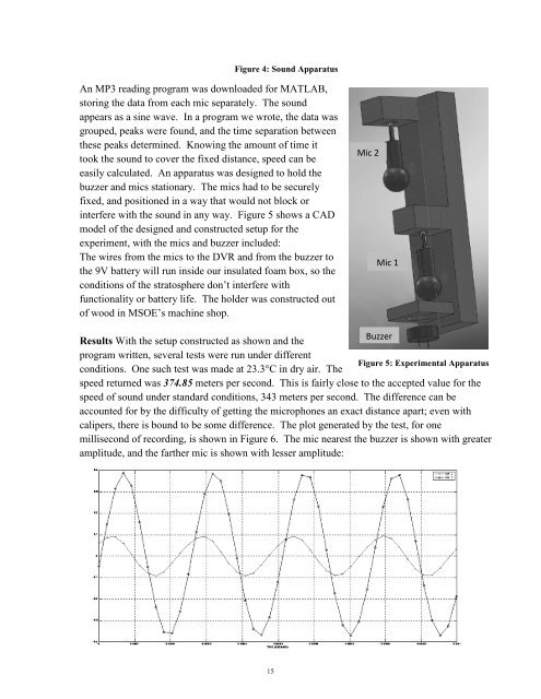
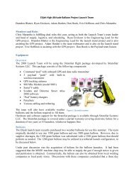
- Page 15 and 16: Elijah High Altitude Balloon Projec
- Page 17 and 18: Our experience with the HALO II lau
- Page 19 and 20: which had been a problem in the pas
- Page 21: Figure 6: 3-D GPS Generated Track o
- Page 24 and 25: Results The seeds tested in the lab
- Page 26 and 27: hour as we assumed the flight in th
- Page 30 and 31: A series of tests were done in a co
- Page 32 and 33: 380 360 340 320 23.3 Temp. (Celsius
- Page 35 and 36: First Place, Non-Engineering: Schmi
- Page 37 and 38: of the basis for fin designs came f
- Page 39 and 40: ejection charge from the motor fire
- Page 41 and 42: using rip-stop nylon cloth. To atta
- Page 43 and 44: Post-flight recovery. A field searc
- Page 45 and 46: Thus, it is believed that the main
- Page 47: [2] Public Missiles Ltd. Frequently
- Page 50 and 51: Design Features The chief requireme
- Page 52 and 53: The joint between the dart and the
- Page 54 and 55: Area dramatically influenced by flo
- Page 56 and 57: Altitude [ft] 6000 5000 4000 3000 2
- Page 58 and 59: though a strong crosswind was prese
- Page 60 and 61: Our Design Our rocket uses the basi
- Page 62 and 63: e easily recovered. Bong recreation
- Page 64 and 65: Performance Characteristics of Pred
- Page 67 and 68: Background and Context: Student Roc
- Page 69 and 70: The Rocky Mountain Miners’ compet
- Page 71: 19th Annual Conference Part Three N
- Page 74 and 75: The angle of repose of a granular m
- Page 76 and 77: Experiment Design The experiment co
- Page 78 and 79:
on the ground and in the Weightless
- Page 80 and 81:
measurements for the 1 − g data.
- Page 82 and 83:
[ImageJ, 2008] Image Analysis Softw
- Page 85 and 86:
Dynamics Characterization of the El
- Page 87 and 88:
Figure 1 - A calibration equation f
- Page 89 and 90:
Wire A secondary investigation into
- Page 91:
[1] Taminger, K. M. B.; and Hafley,
- Page 94 and 95:
Introduction The analysis of wake v
- Page 96 and 97:
Figure 2: Screen I mage o f G UI. T
- Page 98 and 99:
References ¹ Burnham, D.C., and Ha
- Page 101 and 102:
Validation of Novel Rigid Body Fric
- Page 103 and 104:
forces is implemented in the popula
- Page 105 and 106:
Figure 2. CAD representation of a t
- Page 107 and 108:
Results Figure 5. Assembled hydraul
- Page 109:
References Anitescu, M. (2006). "Op
- Page 112 and 113:
Multi-stage Joule-Thomson cycles ar
- Page 114 and 115:
significant change in total compres
- Page 116 and 117:
The enthalpy (h3) of the 2 nd stage
- Page 118 and 119:
UA m� ⎛ ε −1 ⎞ ( c nd c st
- Page 120 and 121:
educed, the temperature range that
- Page 122 and 123:
7. Lemmon, E. W.; Huber, M. L.; McL
- Page 124 and 125:
Throughout each of the run cycles,
- Page 126 and 127:
and heater adjusted to accommodate
- Page 129 and 130:
Phaeton Mast Dynamics Mechanical Sy
- Page 131 and 132:
exposure to the FEMAP with NASTRAN
- Page 133 and 134:
The irregularity in the plots above
- Page 135 and 136:
inversion of a particular matrix, t
- Page 137:
clarified. Additionally, the PMD ki
- Page 140 and 141:
A. Abstract For hardware to be flig
- Page 142 and 143:
should be performed at the JWST obs
- Page 144 and 145:
B. Attenuation and Uncertainty Shoc
- Page 146 and 147:
Detector Array and ROIC SCA Mount L
- Page 148 and 149:
Detector Shock Environment The leve
- Page 150 and 151:
Orbiter (MRO), Moon Mineralogy Mapp
- Page 152 and 153:
4. NASA JPL. MIRI FOCAL PLANE SYSTE
- Page 155 and 156:
Is Lake Superior a significant sour
- Page 157 and 158:
each grid cell at daily resolution.
- Page 159 and 160:
Figure 3. (a) Seasonal cycle of lak
- Page 161 and 162:
Figure 5. Model pCO2 at the surface
- Page 163:
Marshall, J., A. Adcroft, C. Hill,
- Page 166 and 167:
numerical weather prediction (NWP)
- Page 168 and 169:
High Resolution Radiometer (AVHRR)
- Page 170 and 171:
On the morning of 26 May 2008, ther
- Page 172 and 173:
References Behnke, C., 2005: Synopt
- Page 174 and 175:
Figure 3 Figure 3 contains base ref
- Page 177 and 178:
A Comparative Study of Type IIb Sup
- Page 179 and 180:
Fig. 3.— Cartoon Image of SN blas
- Page 181 and 182:
Fig. 4.— Light curve of SN 2008bo
- Page 183:
type IIn Supernova SN 1995N,” 200
- Page 190:
and then can spiral in to the black
- Page 195 and 196:
Understanding the Evolution of Supe
- Page 197 and 198:
Radio
measurements
of
supe
- Page 199 and 200:
In
the
equations
on
the
p
- Page 201 and 202:
SN 2008ax in NGC 4490 SN2008ax is a
- Page 203:
References Chevalier, R. A., “Int
- Page 207 and 208:
Computational Fluid Dynamical Model
- Page 209 and 210:
context of the k − ɛ model invol
- Page 211 and 212:
Figure 3: Experimental results (•
- Page 213 and 214:
direction results in the terminal s
- Page 215:
121 (2000). [Blue Ridge Numerics, I
- Page 218 and 219:
concentrated our effort specificall
- Page 220 and 221:
density, and Ps is a pressure tenso
- Page 222 and 223:
Properties of the GEM problem Recon
- Page 224 and 225:
Figure 1: Increase in reconnection
- Page 226 and 227:
Figure 3: Examples of agreement of
- Page 229 and 230:
Reflection and Refraction of Vortex
- Page 231 and 232:
Experimental Procedure The left han
- Page 233 and 234:
frames in the upper left corner, wh
- Page 235 and 236:
Vortex ring reflection. Similarly,
- Page 237:
References L Bernal and J Kwon. Vor
- Page 240 and 241:
group started in 1997 with the goal
- Page 242 and 243:
I conducted five semi-structured in
- Page 244 and 245:
In the example of the guinea pig pr
- Page 246 and 247:
explain t his t rend. F rom t alkin
- Page 248 and 249:
Research. Washington, DC: Pan Ameri
- Page 250 and 251:
Our team has two goals: 1. To put S
- Page 252 and 253:
fluctuating humidity, drying winds,
- Page 254 and 255:
western border of the Arkansas Rive
- Page 256 and 257:
adjusted to less than .4millisecond
- Page 258 and 259:
Cacti Experiment 18 has produced 10
- Page 260:
13. What N decomposer's are needed
- Page 265 and 266:
Abstract Toxic Offgassing Analysis
- Page 267 and 268:
The chambers were sealed and baked
- Page 269 and 270:
Tables 4 and 5 show offgassing comp
- Page 271:
there was no dichlorobenzene peak.
- Page 274 and 275:
eneficiation reagents. Ionic liquid
- Page 276 and 277:
Figure 3: Current versus voltage da
- Page 279 and 280:
Abstract New Initiatives in the Pro
- Page 281 and 282:
was noticed above the gel. A discol
- Page 283 and 284:
delicate structures (hairs). N o fu
- Page 285:
and A. Y. Rozanov, Eds., SPIE, Vol.
- Page 289 and 290:
Combining Writing Across the Curric
- Page 291 and 292:
But the study also reported a consi
- Page 293 and 294:
Educators’ Aerospace Workshop for
- Page 295 and 296:
2008-2009 Evaluation Educators’ A
- Page 297:
Some comments from participants 200
- Page 300 and 301:
The cost of a one credit graduate c
- Page 303:
EAA WOMEN SOAR - YOU SOAR Dr. Lee J
- Page 306 and 307:
� Incorporated the technology res
- Page 308 and 309:
Evaluation Results: At the conclusi
- Page 310 and 311:
Educational Standards: The National
- Page 312 and 313:
curriculum development, to provide
- Page 314 and 315:
and applications of GIS technology
- Page 316 and 317:
• A significant new outcome for t
- Page 318 and 319:
The design of this project and appl
- Page 320 and 321:
Activities at the workshop involved
- Page 322 and 323:
to give our students a series of PR
- Page 324 and 325:
In the past we have not focused on
- Page 327 and 328:
Providing High School Students with
- Page 329 and 330:
that th e current generations of s
- Page 331:
instruction a s pa rt o f t heir ow
- Page 335 and 336:
Wisconsin Space Grant Consortium &
- Page 337 and 338:
11:45-1:00 pm Lunch *** Concurrent
- Page 339 and 340:
Moderator: David B lock, A ssociate
- Page 341 and 342:
Second Place, E ngineering, Drew an
- Page 343:
Wisconsin Space Grant Consortium