
You also want an ePaper? Increase the reach of your titles
YUMPU automatically turns print PDFs into web optimized ePapers that Google loves.
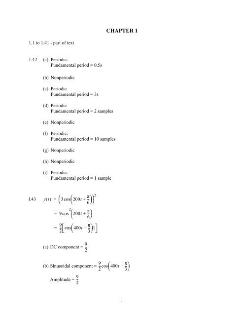
CHAPTER 11.1 to 1.41 - part of text1.42 (a) Periodic:Fundamental period = 0.5s(b) Nonperiodic(c) PeriodicFundamental period = 3s(d) PeriodicFundamental period = 2 samples(e) Nonperiodic(f) Periodic:Fundamental period = 10 samples(g) Nonperiodic(h) Nonperiodic(i) Periodic:Fundamental period = 1 samplel.43πyt () = ⎛3 200t + --⎝cos ⎝⎛ 6⎠⎞ ⎞ 2⎠2π= 9cos⎛200t+ --⎞⎝ 6⎠92-- 400t π= cos + --⎝⎛ 3⎠⎞ 19(a) DC component =--2(b) Sinusoidal component =Amplitude =9--292-- cos 400t π+ --⎝⎛ 3⎠⎞1
Fundamental frequency =200--------Hzπ1.44 The RMS value of sinusoidal x(t) is A ⁄ 2 . Hence, the average power of x(t) in a 1-ohmresistor is ( A ⁄ 2) 2= A 2 /2.1.45 Let N denote the fundamental period of x[N]. which is defined byN=2π-----ΩThe average power of x[n] is thereforePN-11= --- x 2 [ n]N ∑==n=0N-11--- A 2 ⎛ 2πnN ∑ cos⎝ NA 2-----Nn=0N-1∑n=022--------- + φ⎞⎠2πncos ⎛--------- + φ⎞⎝ N ⎠1.46 The energy of the raised cosine pulse isEπ⁄ω 1= ∫-- ( cos( ωt) + 1) 2 dt– π⁄ω41 π⁄ω 2= -- ( cos ( ωt) + 2cos( ωt) + 1) dt2∫01 π⁄ω 11= -- ⎛-- cos( 2ωt)+ -- + 2cos( ωt) + 1⎞ dt2∫0⎝22⎠1= -- 3 2⎝ ⎛ 2 -- ⎠⎞ ⎛---π ⎞ = 3π ⁄ 4ω⎝ω⎠1.47 The signal x(t) is even; its total energy is therefore∫5E = 2 x 2 ()t t d02
∫4= 2 ( 1) 2 dt + 2 ( 5 – t) 2 dt=042[] t t=02= 8 + -- =3+ 226-----3∫541–-- ( 5 – t) 335t=41.48 (a) The differentiator output isyt ()=⎧⎪⎨⎪⎩(b) The energy of y(t) is–41 for – 5 < t < – 4– 1 for 4 < t < 50 otherwiseE = ∫ ( 1) 2 dt + ∫ (–1) 2 dt–54= 1 + 1 = 251.49 The output of the integrator is∫tyt () = A τdτ= At for 0≤t ≤T0Hence the energy of y(t) isE∫T= A 2 t 2 dt=0A 2 T 3------------31.50 (a)x(5t)1.0-1 -0.8 0 0.8 1 t(b)x(0.2t)1.0-25 -20 0 20 25 t3
1.51x(10t - 5)1.00 0.1 0.5 0.9 1.0t1.52 (a)x(t)1-1 1 2 3-1ty(t - 1)-1 1 2 3-1tx(t)y(t - 1)1-1-112 3t4
1.52 (d)x(t)1-3 -2 -1 1 2 3t-1y(1/2t + 1)6 -5 -4 -3 -2 -11 2 4 6-1.0tx(t - 1)y(-t)1-3 -2 -1 1 2 3-1t1.52 (e)x(t)-4 -3 -2 -11-11 2 3ty(2 - t)-4 -3 -2 -11 2 3tx(t)y(2 - t)-1-11 2 3t6
1.52 (f)x(t)1-2 -1 1 2-1ty(t/2 + 1)-6-5-3 -2 -11.01 1 2 3-1.0tx(2t)y(1/2t + 1)+1-1-0.5-11 2t1.52 (g)x(4 - t)-7 -6 -5 -4 -3 -21-1ty(t)-2 -1 1 2 4tx(4 - t)y(t) = 0-3 -2 -1 1 2 3t7
1.53 We may represent x(t) as the superposition of 4 rectangular pulses as follows:g 1 (t)1g 2 (t)1 2 3 4t111 2 3 4g 3 (t)11 2 3 4g 4 (t)tt101 2 3 4To generate g 1 (t) from the prescribed g(t), we letg 1 () t = gat ( – b)where a and b are to be determined. The width of pulse g(t) is 2, whereas the width ofpulse g 1 (t) is 4. We therefore need to expand g(t) by a factor of 2, which, in turn, requiresthat we choose1a = --2The mid-point of g(t)isatt = 0, whereas the mid-point of g 1 (t)isatt = 2. Hence, we mustchoose b to satisfy the conditiona( 2) – b = 0orb = 2a = 2⎛ 1 ⎝2 -- ⎞ = 1⎠Hence, g 1 () t = g⎛1 2 --t – 1 ⎞⎝ ⎠Proceeding in a similar manner, we find thatg 2 () t g 2 3 --t 5= ⎛ – -- ⎞⎝ 3⎠g 3 () t = gt ( – 3)g 4 () t = g( 2t – 7)Accordingly, we may express the staircase signal x(t) in terms of the rectangular pulse g(t)as follows:t8
xt () g⎛ 1 2 --t –⎝1 ⎞ g 2 ⎠ 3 --t 5= + ⎛ – -- ⎞ + gt ( – 3) + g( 2t – 7)⎝ 3⎠1.54 (a)x(t) = u(t) - u(t - 2)(b)(c)-2t0 1 2x(t) = u(t + 1) - 2u(t) + u(t - 1)0 1 2t-1 3-1x(t) = -u(t + 3) + 2u(t +1) -2u(t - 1) + u(t - 3)-301 2 3t-1(d)x(t) = r(t + 1) - r(t) + r(t - 2)1-2 -1 0 1 2 3t(e)x(t) = r(t + 2) - r(t + 1) - r(t - 1)+ r(t - 2)1-3 -2 -1 0 1 2t9
1.55 We may generate x(t) as the superposition of 3 rectangular pulses as follows:g 1 (t)1-4 -2 0 2 4g 2 (t)1-4 -2 0 2 4g 3 (t)1ttAll three pulses, g 1 (t), g 2 (t), and g 3 (t), are symmetrically positioned around the origin:1. g 1 (t) is exactly the same as g(t).2. g 2 (t) is an expanded version of g(t) by a factor of 3.3. g 3 (t) is an expanded version of g(t) by a factor of 4.Hence, it follows thatg 1 () t = gt ()g 2() t = g⎛1 ⎝3 --t ⎞⎠g 3 () t = g⎛1 ⎝4 --t ⎞⎠That is,xt () = gt () + g⎛ 1 ⎝3 --t ⎞ + g⎛1⎠ ⎝4 --t ⎞⎠-4 - 2 0 2 4t1.56 (a)o2x[2n]o(b)o-1 0 1x[3n - 1]2 ono 1o-1 0 1n10
1.56 (c)y[1 - n]o o o o o 1-4 -3 -2 -1 0-1o12 3 4 5o o o on(d)y[2 - 2n]o o o o 1-3 -2 -1-1o12 3 4 5o o o on(e)x[n - 2] + y[n + 2]o4oo 3o2oo-7 -6 -5 -4 -3o o o o o1 oo o oo-2 -1 0 1 2 3 4 5 6 7 8n(f)x[2n] + y[n - 4]o 1 oo o o-5 -4 -3 -2 2 3o-1 4 5 6 7o o o o o -1 o on11
1.56 (g)x[n + 2]y[n - 2]o-5 -4 -3 -2 -1 1ooonoo1oo 2o3o(h)x[3 - n]y[-n]3o2 oo1 o oo o oo o-3 -2 -1 1 2 3 4 5 6 7 8n(i)ox[-n] y[-n]3o2oo o-5 -4 -3 -2 -11o1 2 3 4o5o6o-1 on-2o(j)-3ox[n]y[-2-n]o32o o o-6 -5 -4 -31-2 -1o o1 2 3 4o5o6oo -1 o-2 o-3 on12
1.56 (k)x[n + 2]y[6-n]3o2-8o-7o-6 -5 -4o-3oo 1o-2 -1-1o o o o o1 2 3 4 5 6no-2o-31.57 (a) PeriodicFundamental period = 15 samples(b) PeriodicFundamental period = 30 samples(c) Nonperiodic(d) PeriodicFundamental period = 2 samples(e) Nonperiodic(f) Nonperiodic(g) PeriodicFundamental period = 2π seconds(h) Nonperiodic(i) PeriodicFundamental period = 15 samples1.58 The fundamental period of the sinusoidal signal x[n] isN = 10. Hence the angularfrequency of x[n] is2πmΩ = ---------- m: integerNThe smallest value of Ω is attained with m = 1. Hence,2π πΩ = ----- = -- radians/cycle10 513
1.59 The amplitude of complex signal x(t) is defined by2 2 2x R() t + xI () t = A cos2( ωt + φ) + A 2 sin ( ωt + φ)2==2A cos ( ωt + φ) + sin ( ωt + φ)A21.60 Real part of x(t) isRe{ xt ()} = Ae αt cos( ωt)Imaginary part of x(t) isIm{ xt ()} = Ae αt sin( ωt)1.61 We are givenxt ()=⎧ t ∆ ∆⎪ -- for –-- ≤t≤ --⎪ ∆ 2 2⎪ ∆⎨ 1 for t ≥ --⎪ 2⎪⎪∆2 for t < –--⎩2The waveform of x(t) is as followsx(t)112-∆/20∆/2t-1214
The output of a differentiator in response to x(t) has the corresponding waveform:y(t)11/∆2 δ(t - 12)-∆/2 0 ∆/2t12 δ(t + ∆2)y(t) consists of the following components:1. Rectangular pulse of duration ∆ and amplitude 1/∆ centred on the origin; the areaunder this pulse is unity.2. An impulse of strength 1/2 at t = ∆/2.3. An impulse of strength -1/2 at t = -∆/2.As the duration ∆ is permitted to approach zero, the impulses (1/2)δ(t-∆/2) and-(1/2)δ(t+∆/2) coincide and therefore cancel each other. At the same time, the rectangularpulse of unit area (i.e., component 1) approaches a unit impulse at t = 0. We may thus statethat in the limit:lim∆ → 0yt ()==lim∆ → 0δ()t----x d () tdt1.62 We are given a triangular pulse of total duration ∆ and unit area, which is symmetricalabout the origin:x(t)2/∆slope = 4/∆ 2slope = -4/∆ 2area = 1-∆/2 0 ∆/2t15
(a) Applying x(t) to a differentiator, we get an output y(t) depicted as follows:y(t)area = 2/∆4/∆ 2 ∆/2-∆/2-4/∆ 2area = 2/∆t(b) As the triangular pulse duration ∆ approaches zero, the differentiator outputapproaches the combination of two impulse functions described as follows:• An impulse of positive infinite strength at t = 0 - .• An impulse of negative infinite strength at t = 0 + .(c) The total area under the differentiator output y(t) is equal to (2/∆) + (-2/∆) = 0.In light of the results presented in parts (a), (b), and (c) of this problem, we may now makethe following statement:When the unit impulse δ(t) is differentiated with respect to time t, the resulting outputconsists of a pair of impulses located at t =0 - and t =0 + , whose respective strengthsare +∞ and -∞.1.63 From Fig. P.1.63 we observe the following:x 1 () t = x 2 () t = x 3 () t = xt ()x 4() t = y 3() tHence, we may writey 1 () t = xt ()xt ( – 1)y 2() t = xt ()y 4 () t = cos( y 3 () t ) = cos( 1 + 2x()t)The overall system output isyt () = y 1 () t + y 2 () t – y 4 () tSubstituting Eqs. (1) to (3) into (4):yt () = xt ()xt ( – 1) + xt ()–cos( 1 + 2xt ())(1)(2)(3)(4)(5)Equation (5) describes the operator H that defines the output y(t) in terms of the input x(t).16
1.64 Memoryless Stable Causal Linear Time-invariant(a) ✓ ✓ ✓ x ✓(b) ✓ ✓ ✓ ✓ ✓(c) ✓ ✓ ✓ x ✓(d) x ✓ ✓ ✓ ✓(e) x ✓ x ✓ ✓(f) x ✓ ✓ ✓ ✓(g) ✓ ✓ x x ✓(h) x ✓ ✓ ✓ ✓(i) x ✓ x ✓ ✓(j) ✓ ✓ ✓ ✓ ✓(k) ✓ ✓ ✓ ✓ ✓(l) ✓ ✓ ✓ x ✓1.65 We are givenyn [ ] = a 0xn [ ] + a 1xn [ – 1] + a 2xn [ – 2] + a 3xn [ – 3](1)LetS k { xn ( )} = xn ( – k)We may then rewrite Eq. (1) in the equivalent formyn [ ] = a 0xn [ ] + a 1S 1 { xn [ ]} + a 2S 2 { xn [ ]} + a 3S 3 { xn [ ]}= ( a 0+ a 1S 1 + a 2S 2 + a 3S 3 ){ xn [ ]}= H{ x[ n]}whereH = a 0 + a 1 S 1 + a 2 S 2 + a 3 S 3(a) Cascade implementation of operator H:x[n]. . .S S Sa 0 a 1 a 2 a 3Σy[n]17
(b) Parallel implementation of operator H:x[n]. ..a 0S 1a 1Σ y[n]S 2a 2S 3 a 31.66 Using the given input-output relation:yn [ ] = a 0 xn [ ] + a 1 xn [ – 1] + a 2 xn [ – 2] + a 3 xn [ – 3]we may writeyn [ ] = a 0 xn [ ] + a 1 xn [ – 1] + a 2 xn [ – 2] + a 3 xn [ – 3]≤ a 0xn [ ] + a 1xn [ – 1] + a 2xn [ – 2] + a 3xn [ – 3]≤ a 0 M x + a 1 M x + a 2 M x + a 3 M x= ( a 0 + a 1 + a 2 + a 3 )M xwhere M x= xn ( ) . Hence, provided that M x is finite, the absolute value of the outputwill always be finite. This assumes that the coefficients a 0 , a 1 , a 2 , a 3 have finite values oftheir own. It follows therefore that the system described by the operator H of Problem 1.65is stable.1.67 The memory of the discrete-time described in Problem 1.65 extends 3 time units into thepast.1.68 It is indeed possible for a noncausal system to possess memory. Consider, for example, thesystem illustrated below:x[n]x(n + k) S kS l. .x(n - l)a k a 0 a lΣThat is, with S l {x[n]} = x[n - l], we have the input-output relationyn [ ] = a 0 xn [ ] + a k xn [ + k] + a l xn [ – l]This system is noncausal by virtue of the term a k x[n + k]. The system has memory byvirtue of the term a l x[n - l].y[n]18
1.69 (a) The operator H relating the output y[n] to the input x[n] isH = 1 + S 1 + S 2whereS k { xn [ ]} = xn [ – k]for integer k(b) The inverse operator H inv is correspondingly defined byH inv = --------------------------11 + S 1 + S 2Cascade implementation of the operator H is described in Fig. 1. Correspondingly,feedback implementation.of the inverse.operator H inv is described in Fig. 2x[n]SSFig. 1Operator HFigure 2 follows directly from the relation:xn [ ] = yn [ ] – xn [ – 1]– xn [ – 2]1.70 For the discrete-time system (i.e., the operator H) described in Problem 1.65 to be timeinvariant,the following relation must holdS n0 H = HS n 0for integer n 0 (1)whereS n 0{ xn [ ]} = xn [ – n 0 ]andH = 1 + S 1 + S 2We first note thatS n 0= + +Next we note thaty[n]Fig. 2Inverse Operator H invS n0 H = S n0 ( 1 + S 1 + S 2 )HS n 0=S n 0 + 1(1 S 1 S 2 + + )S n 0+S n 0 + 2Σ--Σ.S Sy[n].x[n](2)19
S n 0S 1 + n 0S 2 + n 0= + +(3)From Eqs. (2) and (3) we immediately see that Eq. (1) is indeed satisfied. Hence, thesystem described in Problem 1.65 is time-invariant.1.71 (a) It is indeed possible for a time-variant system to be linear.(b) Consider, for example, the resistance-capacitance circuit where the resistivecomponent is time variant, as described here:This circuit, consisting of the series combination of the resistor R(t) and capacitor C, istime variant because of R(t).The input of the circuit, v 1 (t), is defined in terms of the output v 2 (t) byv 1 () t Rt ()C dv 2= -------------- () t+ vdt 2 () tDoubling the input v 1 (t) results in doubling the output v 2 (t). Hence, the property ofhomogeneity is satisfied.Moreover, ifv 1 () t = v 1, k () tthenN∑k=1N∑v 2() t = v 2, k() tk=1v 1 (t)wherev 1, k () t Rt ()C dv 2, k()t= ------------------- + v , k = 1,2,...,Ndt 2, k () tHence, the property of superposition is also satisfied.+.R(t)i(t)C.We therefore conclude that the time-varying circuit of Fig. P1.71 is indeed linear.o +o -v 2 (t)1.72 We are given the pth power law device:yt () = x p () t(1)20
Let y 1 (t) and y 2 (t) be the outputs of this system produced by the inputs x 1 (t) and x 2 (t),respectively. Let x(t) =x 1 (t) +x 2 (t), and let y(t) be the corresponding output. We then notethatyt () = ( x 1() t + x 2() t ) p ≠ y 1() t + y 2() t for p ≠ 01 ,Hence the system described by Eq. (1) is nonlinear.1.73 Consider a discrete-time system described by the operator H 1 :H 1:yn [ ] = a 0xn [ ] + a kxn [ – k]This system is both linear and time invariant. Consider another discrete-time systemdescribed by the operator H 2 :H 2:yn [ ] = b 0xn [ ] + b kxn [ + k]which is also both linear and time invariant. The system H 1 is causal, but the secondsystem H 2 is noncausal.1.74 The system configuration shown in Fig. 1.56(a) is simpler than the system configurationshown in Fig. 1.56(b). They both involve the same number of multipliers and summer.however, Fig. 1.56(b) requires N replicas of the operator H, whereas Fig. 1.56(a) requires asingle operator H for its implementation.1.75 (a) All three systems• have memory because of an integrating action performed on the input,• are causal because (in each case) the output does not appear before the input, and• are time-invariant.(b) H 1 is noncausal because the output appears before the input. The input-output relationof H 1 is representative of a differentiating action, which by itself is memoryless.However, the duration of the output is twice as long as that of the input. This suggeststhat H 1 may consist of a differentiator in parallel with a storage device, followed by acombiner. On this basis, H 1 may be viewed as a time-invariant system with memory.System H 2 is causal because the output does not appear before the input. The durationof the output is longer than that of the input. This suggests that H 2 must have memory.It is time-invariant.System H 3 is noncausal because the output appears before the input. Part of the output,extending from t =-1tot = +1, is due to a differentiating action performed on theinput; this action is memoryless. The rectangular pulse, appearing in the output fromt =+1tot = +3, may be due to a pulse generator that is triggered by the termination ofthe input. On this basis, H 3 would have to be viewed as time-varying.21
Finally, the output of H 4 is exactly the same as the input, except for an attenuation by afactor of 1/2. Hence, H 4 is a causal, memoryless, and time-invariant system.1.76 H 1 is representative of an integrator, and therefore has memory. It is causal because theoutput does not appear before the input. It is time-invariant.H 2 is noncausal because the output appears at t = 0, one time unit before the delayed inputat t = +1. It has memory because of the integrating action performed on the input. But,how do we explain the constant level of +1 at the front end of the output, extending fromt =0tot = +1? Since the system is noncausal, and therefore operating in a non real-timefashion, this constant level of duration 1 time unit may be inserted into the output byartificial means. On this basis, H 2 may be viewed as time-varying.H 3 is causal because the output does not appear before the input. It has memory because ofthe integrating action performed on the input from t =1tot = 2. The constant levelappearing at the back end of the output, from t =2tot = 3, may be explained by thepresence of a strong device connected in parallel with the integrator. On this basis, H 3 istime-invariant.Consider next the input x(t) depicted in Fig. P1.76b. This input may be decomposed intothe sum of two rectangular pulses, as shown here:x(t) x A (t) x B (t)2121+210 1 2 t 0 1 2 t 0 1 2 tResponse of H 1 to x(t):y 1,A (t) y 1,B (t) y 1 (t)21+21210 1 2 t 0 1 2 t0 1 2 t22
Response of H 2 to x(t):y 2,A (t)y 2,B (t)y 2 (t)21-1 0-1+11 2t0 1-12t2-1 0 1-12t-2-2The rectangular pulse of unit amplitude and unit duration at the front end of y 2 (t) isinserted in an off-line manner by artificial meansResponse of H 3 to x(t):y 3,A (t)y 3,B (t)3y 3 (t)21+21210 1 2 t 0 1 2 3 t 0 1 2 3 t1.77 (a) The response of the LTI discrete-time system to the input δ[n-1] is as follows:y[n]2 o1o2 4 5o oo o n-1 1 3-1 o(b) The response of the system to the input 2δ[n] - δ[n - 2] is as followsy[n]4o321o14o o o o o-2 -1 0 2 3 5 6-1o-2 on23
(c) The input given in Fig. P1.77b may be decomposed into the sum of 3 impulsefunctions: δ[n + 1], -δ[n], and 2δ[n - 1]. The response of the system to these threecomponents is given in the following table:Timenδ[n + 1] -δ[n] 2δ[n - 1] Totalresponse-10123+2-1+1-2+1-1+4-2+2+1-3+6-32Thus, the total response y[n] of the system is as shown here:y[n]6 o5432oo 12 4 5 6o oo o o-3 -2 -1 0 1 3-1-2-3 ooAdvanced Problems1.78 (a) The energy of the signal x(t) is defined byE=∫∞–∞x 2 ()t t dSubstitutingxt () = x e () t + x o () tinto this formula yieldsE ===∫∫∫∞–∞∞–∞∞–∞[ x e() t + x o() t ] 2 dt2 2[ x e() t + xo() t + 2xe ()x t o () t ] 2 dt2x e()tt d + ∫∞ 2 xo t–∞∫∞()t d + 2 xe ()x t o ()t t d–∞(1)24
With x e (t) even and x o (t) odd, it follows that the product x e (t)x o (t) is odd, as shown byx e(–t)x o (–t) = x e () t [–x o () t ]= – x e()x t o() tHence,∫∞–∞( x e ()x t o () t ) dt=–∞Accordingly, Eq. (1) reduces toE=∫∞–∞2x e()tt d + ∫===∞–∞∫∫00–∞– ∫0∞0x e ()x t o ()t t d+ ∫∞0x e ()x t o ()t t d(– x e ()x t o () t )(–dt) + ∫ ( x e ()x t o () t ) dt2 xo()tt dx e ()x t o ()t t d+ ∫∞0∞0x e ()x t o ()t t d(b) For a discrete-time signal x[n],E===∞∑n=-∞∞∑n=-∞∞∑n=-∞x 2 [ n][ x e[ n] + x o[ n]] 2∞∑2 2 2x e[ n]+ xo[ n]+ 2 x e [ n]x o [ n]n=-∞– ∞ ≤n≤ ∞, we may similarly write∞∑n=-∞(2)Withx e [–n]x o [–n] = – x e [ n]x o [ n]it follows that∞∑n=-∞x e [ n]x o [ n]==== 00∑n=-∞0∑ x en=-∞0– ∑n=∞x e [ n]x o [ n] + x e [ n]x o [ n][–n]x o – n∞∑n=-0∞∑[ ] + x e [ n]x o [ n]n=-0∞∑x e [ n]x o [ n] + x e [ n]x o [ n]n=025
Accordingly, Eq. (2) reduces toE =∞∑n=-∞∞∑2 2x e[ n]+ xo[ n]n=-∞1.79 (a) From Fig. P1.79,it () = i 1() t + i 2() tL di 1------------- () t+ Ridt 1() t =1 t--- iC∫2( τ) dτ–∞(1)(2)Differentiating Eq. (2) with respect to time t:L d2 ---------------- i 1() tdt 2 R di1()t 1+ ------------- = ---idt C 2() t(3)Eliminating i 2 (t) between Eqs. (1) and (2):L d2 ---------------- i 1 () tdt 2 + R -------------di1()tdt=1--- [ it ()–iC 1() t ]Rearranging terms:d 2 i 1() t---------------- -- R di1()t 1dt 2 + ------------- + ------- iL dt LC 1() t=1------- it ()LC(4)(b) Comparing Eqs. (4) with Eq. (1.108) for the MEMS as presented in the text, we mayderive the following analogy:MEMS of Fig. 1.64 LRC circuit of Fig. P1.79y(t)ω ni 1 (t)1 ⁄ LCQω n L---------R=1--RL---Cx(t)1------- it ()LC26
1.80 (a) As the pulse duration ∆ approaches zero, the area under the pulse x ∆ (t) remains equalto unity, and the amplitude of the pulse approaches infinity.(b) The limiting form of the pulse x ∆ (t) violates the even-function property of the unitimpulse:δ( – t) = δ()t1.81 The output y(t) is related to the input x(t) asyt () = H{ x()t }(1)Let T 0 denote the fundamental period of x(t), assumed to be periodic. Then, by definition,xt () = xt ( + T 0 )(2)Substituting t +T 0 for t into Eq. (1) and then using Eq. (2), we may writeyt ( + T 0) = H{ x( t + T 0)}= H{ x()t }= yt ()(3)Hence, the output y(t) is also periodic with the same period T 0 .1.82 (a) For 0 ≤ t < ∞ , we havex ∆() t=1-- e – t ⁄ τ∆At t = ∆/2, we haveA = x ∆( ∆ ⁄ 2)1= -- e – ∆ ⁄ ( 2τ)∆Since x ∆ (t) is even, thenA = x ∆ ( ∆ ⁄ 2) = x ∆ (– ∆ ⁄ 2)=1-- e – ∆ ⁄ 2τ∆( )(b) The area under the pulse x ∆ (t) must equal unity forδ() t = lim x ∆ () t∆ → 0The area under x ∆ (t) is27
∞∫ x ∆()t t d = 2∫x ∆()t t d–∞=2∫0∞0∞1-- e t ⁄ τ∆– dt2= -- (–τ)e t ⁄ τ∆2τ= -----∆– 0∞For this area to equal unity, we require∆τ = --2(c)876∆ = 1∆ = 0.5∆ = 0.25∆ = 0.1255Amplitude43210−2 −1.5 −1 −0.5 0 0.5 1 1.5 2Time1.83 (a) Let the integral of a continuous-time signal x(t), – ∞ < t < ∞ , be defined by∫tyt () = x( τ) dτ=∫–∞0–∞xt ()t d + ∫t0x( τ) dτ28
The definite integral∫0–∞xt ()t d , representing the initial condition, is a constant.With differentiation as the operation of interest, we may also writedy()txt () = ------------dtClearly, the value of x(t) is unaffected by the value assumed by the initial condition∫0–∞xt ()t dIt would therefore be wrong to say that differentiation and integration are the inverseof each other. To illustrate the meaning of this statement, consider the two followingtwo waveforms that differ from each other by a constant value for – ∞ < t < ∞ :x 1 (t)x 2 (t)slope = aslope = a0 t 0 tYet,yt ()dx 1 () t= --------------- =dtdx 2 () t--------------- , as illustrated below:dty(t)a0 t(b) For Fig. P1.83(a):R tyt () + -- y( τ) dτL∫= xt ()–∞For R/L large, we approximately haveR t-- y( τ) dτ≈xt ()L∫–∞Equivalently, we have a differentiator described byyt () -- L dx()t R≈ ------------ , -- largeR dt L29
For Fig. P1.83(b):Lyt () + -- dy ------------() t = xt ()R dtFor R/L small, we approximately haveL-- ------------ dy()t ≈ xt ()R dtEquivalently, we have an integrator described byR tRyt () ≈ -- x( τ) dτsmallL∫--L–∞(c) Consider the following two scenarios describing the LR circuits of Fig. P1.83• The input x(t) consists of a voltage source with an average value equal to zero.• The input x(t) includes a dc component E (exemplified by a battery).These are two different input conditions. Yet for large R/L, the differentiator of Fig.P1.83(a) produces the same output. On the other hand, for small R/L the integrator ofFig. P1.83(b) produces different outputs. Clearly, on this basis it would be wrong tosay that these two LR circuits are the inverse of each other.1.84 (a) The output y(t) is defined byyt () = A 0cos( ω 0t + φ)xt()(1)This input-output relation satisfies the following two conditions:• Homogeneity: If the input x(t) is scaled by an arbitrary factor a, the output y(t) willbe scaled by the same factor.• Superposition: If the input x(t) consists of two additive components x 1 (t) and x 2 (t),thenyt () = y 1() t + y 2() twhereyt () = A 0 cos( ω 0 t + φ)x k () t , k = 1,2Hence, the system of Fig. P1.84 is linear.(b) For the impulse inputxt () = δt (),Eq. (1) yields the corresponding outputy′ () t = A 0cos( ω 0t + φ)δ()t30
=⎧⎨⎩A 0 cosφδ( 0),t = 00, otherwiseFor xt () = δt ( – t 0), Eq. (1) yieldsy″ () t = A 0cos( ω 0t + φ)δ( t – t 0)=⎧⎨⎩A 0 cos( ω 0 t 0 + φ)δ( 0),t = t 00, otherwiseRecognizing thaty′ () t ≠ y″ () t , the system of Fig. P1.84 is time-variant.1.85 (a) The output y(t) is related to the input x(t) asyt () = cos 2π f ct + k∫x( τ) dτ⎝⎛ ⎠⎞t–∞(1)The output is nonlinear as the system violates both the homogeneity and superpositionproperties:• Let x(t) be scaled by the factor a. The corresponding value of the output isy a () t = cos 2π f c t + ka∫x( τ) dτ⎝⎛ ⎠⎞For a ≠ 1 , we clearly see that y a () t ≠ yt ().• Letxt () = x 1() t + x 2() tThenyt () = cos 2π f ct + k∫x 1( τ) dτ + k∫x 2( τ) dτ⎝⎛ –∞–∞ ⎠⎞≠ y 1 () t + y 2 () twhere y 1 (t) and y 2 (t) are the values of y(t) corresponding to x 1 (t) and x 2 (t),respectively.(b) For the impulse inputxt () = δt (),Eq. (1) yieldstt–∞y′ () t = cos 2π f ct + k∫δτ ( ) dτ⎝⎛ ⎠⎞t–∞t31
= cosk,t = 0 +For the delayed impulse inputxt () = δt ( – t 0), Eq. (1) yieldsy″ () t = cos 2π f ct + k∫δτ ( – t 0) dτ⎝⎛ ⎠⎞–∞+= cos( 2π f c t 0 + k), t = t 0tRecognizing thaty′ () t ≠ y″ () t , it follows that the system is time-variant.1.86 For the square-law deviceyt () = x 2 () t ,the inputxt () = A 1 cos( ω 1 t + φ 1 ) + A 2 cos( ω 2 t + φ 2 )yields the outputyt () = x 2 () t= [ A 1cos( ω 1t + φ 1) + A 2cos( ω 2t + φ 2)] ==2A 2 21 cos ( ω 1 t + φ 1 ) + A 2 2 cos ( ω 2 t + φ 2 )+ 2A 1 A 2 cos( ω 1 t + φ 1 ) cos( ω 2 t + φ 2 )A 12----- [ 1 + cos( 2ω21 t + 2φ 1 )]A 22+ ----- [ 1+cos( 2ω22 t + 2φ 2 )]+ A 1 A 2 [ cos( ( ω 1 + ω 2 )t + ( φ 1 + φ 2 )) + cos( ( ω 1 – ω 2 )t + ( φ 1 – φ 2 ))]The output y(t) contains the following components:• DC component of amplitude ( + ) ⁄ 22• Sinusoidal component of frequency 2ω 1 , amplitude A 1 ⁄ 2 , and phase 2φ 12• Sinusoidal component of frequency 2ω 2 , amplitude A 2 ⁄ 2 , and phase 2φ 2• Sinusoidal component of frequency (ω 1 - ω 2 ), amplitude A 1 A 2 , and phase (φ 1 - φ 2 )• Sinusoidal component of frequency (ω 1 + ω 2 ), amplitude A 1 A 2 , and phase (φ 1 + φ 2 )1.87 The cubic-law deviceyt () = x 3 () t ,in response to the input,A 12A 2232
xt () = Acos( ωt + φ),produces the outputyt () = A 3 3cos ( ωt + φ)= A 3 3 1cos ( ωt + φ)⋅ -- ( cos( ( 2ωt + 2φ) + 1))2=A-----[ 3cos( ( 2ωt + 2φ) + ( ωt + φ))2==+ cos( ( 2ωt + 2φ) – ( ωt + φ))]A 3----- [ cos( 3ωt + 3φ) + cos( ωt + φ)] +2A 3----- cos( 3ωt + 3φ) + A 3 cos( ωt + φ)2The output y(t) consists of two components:• Sinusoidal component of frequency ω, amplitude A 3 and phase φ• Sinusoidal component of frequency 3ω, amplitude A 3 /2, and phase 3φTo extract the component with frequency 3ω (i.e., the third harmonic), we need to use aband-pass filter centered on 3ω and a pass-band narrow enough to suppress thefundamental component of frequency ω.From the analysis presented here we infer that, in order to generate the pth harmonic inresponse to a sinusoidal component of frequency ω, we require the use of two subsystems:• Nonlinear device defined byyt () = x p () t , p = 2,3,4,...• Narrowband filter centered on the frequency pω.+A 3----- cos( ωt + φ)2A 3----- cos( ωt + φ)21.88 (a) Following the solution to Example 1.21, we start with the pair of inputs:x 1 () tx 2() t==1∆-- u ⎛⎝t1∆-- u ⎛⎝t∆+ -- ⎞2⎠∆– -- ⎞2⎠The corresponding outputs are respectively given by33
y 1 () ty 2 () t==∆– α⎛t+ -- ⎞1 ⎝ 2⎠∆-- 1 – e cosω ⎛∆n t + -- ⎞ u⎛t⎝ 2⎠⎝∆– α⎛t– -- ⎞1 ⎝ 2⎠∆-- 1 – e cosω ⎛∆n t – -- ⎞ u⎛t⎝ 2⎠⎝∆+ -- ⎞2⎠∆– -- ⎞2⎠The response to the inputx ∆() t = x 1() t – x 2() tis given byy ∆() t1∆-- ⎧u ⎛ t ∆+ -- ⎞ ∆=u⎛t– -- ⎞⎨ –⎝ 2⎠⎝ 2⎠⎩⎧1 ⎪– -- e∆⎨⎪⎩∆– α⎛t+ -- ⎞⎝ 2⎠ωω nt n∆cos + ---------⎝⎛ 2 ⎠⎞ ∆ u ⎛ t + -- ⎞⎝ 2⎠– e∆– α⎛t– -- ⎞⎝ 2⎠ωω nt n ∆cos – ---------⎝⎛ 2 ⎠⎞ ∆ u ⎛ t – -- ⎞⎝ 2⎠⎫⎪⎬⎪⎭As∆ → 0,x ∆ () t → δt (). We also note thatd----z()tdt=⎧1∆-- z ⎛ t ∆+ -- ⎞ ∆limz⎛t– -- ⎞⎨ –→ ⎝ 2⎠⎝ 2⎠⎩∆ 0⎫⎬⎭Hence, with zt () = e αt cos( ω t )ut (), we find that the impulse response of thesystem isyt () = lim y ∆ () t∆ → 0d= δ()t – ---- [ e – αt cos( dtω t )ut ()]nd= δ()t – ---- [ e – αt cos( ωdtn t)] ⋅ ut ()–[ e – αt cos( ω n t)]----u d () tdt–αt= δ() t – [–αe cos( ω n t) – ω n e – αt sin( ω n t)]ut ()–– cos( ω t )δ()t ne αt(1)34
Since e – αt cos( ω nt)= 1 at t = 0, Eq. (1) reduces toyt () = [ αe – αt cos( ω t ) + ω n ne – αt sin( ω nt)]ut ()(2)(b)ω n= jα n where α n < αUsing Euler’s formula, we can writecos( ω nt)e jω nte – jωnt+= ------------------------------ =2e – α nt+ e α nt--------------------------2The step response can therefore be rewritten as1 –(yt () 1 -- e α + α n)t–(e α – α n)t= – ( + ) ut ()2Again, the impulse response in this case can be obtained asht ()dy()t 1 –(------------ 1 -- e α + α n)t–(e α – α n)t= = – ( + ) δ()tdt 2+⎧ ⎪⎪⎪⎪⎪⎨⎪⎪⎪⎪⎪⎩= 0α+α n –( ---------------e α + α n)tα–α n –(---------------e α – α n)t+ ut ()22=α 2-----e α 2t2– α 1–-----e α 1t+ ut ()2where α 1 = α - α n and α 2 = α + α n .1.89 Building on the solution described in Fig. 1.69, we may relabel Fig. P1.89 as follows.x[n] +y′[n]+ΣΣ y[n]++where (see Eq. (1.117))andyn [ ] = y′ [ n] + 0.5y′ [ n – 1].0.5 S 0.5y′ [ n] = xn [ ] + 0.5 k xn [ – k]∞∑k=135
==∞xn [ ] + ∑ 0.5 k xn [ – k ] + 0.5x[ n–1] + ∑ 0.5 k xn [ – 1 – k]∞k=1∑ 0.5 k xn [ – k ] + 0.5∑0.5 k xn [ – 1 – k]k=0∞k=0∞k=11.90 According to Eq. (1.108) the MEMS accelerometer is described by the second-orderequationd 2 yt () ω-------------- ----- n 2 + ------------ +dt 2ωQ dt nyt() = xt ()(1)Next, we use the approximation (assuming that T s is sufficiently small)d----y()tdt≈T s1T ---- y ⎛ t + ----⎞ – y⎛ts⎝ 2 ⎠ ⎝T s– ----⎞2 ⎠Applying this approximation a second time:d 2 yt () 1--------------dt 2 ≈ ----T s=1----T sddt---- y ⎝tT sT s⎛ + ----⎞ – y⎛t– ----⎞2 ⎠ ⎝ 2 ⎠T sddt----y ⎛ t + ----⎞ 1– ----⎝ 2 ⎠T sddt----y ⎛⎝t1 ⎧ 1⎫≈ ---- ---- yt TT⎨ [ ( +sT s)–yt ()]⎬⎩ s⎭T s– ----⎞2 ⎠(2)1 ⎧ 1⎫– ---- ---- yt () yt TT⎨ [ – ( –s T s)]⎬⎩ s⎭1= ----- [ yt ( + T s) – 2y()t + yt ( – T s)]T s2Substituting Eqs. (2) and (3) into (1):1----- [ yt ( + T s ) – 2y()t + yt ( – T s )]QT --------- y ⎛ t + ----⎞ y⎛t– ----⎞2 + – + ωs⎝ 2 ⎠ ⎝ 2 ⎠ nyt() = xt ()T s2ω n2T sT s(3)(4)Define2ω nT ----------- sQ= a 1 ,2 2ω nT s – 2 = a 2 ,36
1----- = b ,2 0T st = nT s⁄ 2 ,yn [ ] = ynT ( s⁄ 2),where, in effect, continuous time is normalized with respect to T s /2 to get n.We may then rewrite Eq. (4) in the form of a noncausal difference equation:yn [ + 2] + a 1yn [ + 1] + a 2yn [ ] – a 1yn [ – 1] + yn [ – 2]= b 0xn [ ](5)Note: The difference equation (5) is of order 4, providing an approximate description of asecond-order continuous-time system. This doubling in order is traced to Eq. (2) as theapproximation for a derivative of order 1. We may avoid the need for this order doublingby adopting the alternative approximation:d----y()tdt1≈ ---- [ yt ( + T s )–yt ()]T sHowever, in general, for a given sampling period T s , this approximation may not be asaccurate as that defined in Eq. (2).1.91 Integration is preferred over differentiation for two reasons:(i) Integration tends to attenuate high frequencies. Recognizing that noise contains abroad band of frequencies, integration has a smoothing effect on receiver noise.(ii) Differentiation tends to accentuate high frequencies. Correspondingly, differentiationhas the opposite effect to integration on receiver noise.1.92 From Fig. P1.92, we haveit () = i 1 () t + i 2 () tvt () = Ri 2() t =1 t--- iC∫1( τ) dτ–∞This pair of equations may be rewritten in the equivalent form:1i 1 () t = it ()–-- vt ()Rvt ()1 t= --- iC∫1 ( τ) dτ–∞37
Correspondingly, we may represent the parallel RC circuit of Fig. P1.92 by the blockdiagram.i(t) i 1 (t) 1 t v(t)Σ--- dτ+C∫–∞-The system described herein is a feedback system with the capacitance C providing theforward path and the conductance 1/R providing the feedback path.1R%Solution to Matlab Experiment 1.93f = 20;k = 0:0.0001:5/20;amp = 5;duty = 60;%Make Square Wavey1 = amp * square(2*pi*f*k,duty);%Make Sawtooth Wavey2 = amp * sawtooth(2*pi*f*k);%Plot Resultsfigure(1); clf;subplot(2,1,1)plot(k,y1)xlabel(’time (sec)’)ylabel(’Voltage’)title(’Square Wave’)axis([0 5/20 -6 6])subplot(2,1,2)plot(k,y2)xlabel(’time (sec)’)ylabel(’Voltage’)title(’Sawtooth Wave’)38
axis([0 5/20 -6 6])6Square Wave42Voltage0−2−4−60 0.05 0.1 0.15 0.2 0.25time (sec)6Sawtooth Wave42Voltage0−2−4−60 0.05 0.1 0.15 0.2 0.25time (sec)% Solution to Matlab Experiment 1.94t = 0:0.01:5;x1 = 10*exp(-t) - 5*exp(-0.5*t);x2 = 10*exp(-t) + 5*exp(-0.5*t);%Plot Figuresfigure(1); clf;subplot(2,1,1)plot(t,x1)xlabel(’time (sec)’)ylabel(’Amplitude’)title(’x(t) = e^{-t} - e^{-0.5t}’)subplot(2,1,2);plot(t,x2)xlabel(’time (sec)’)ylabel(’Amplitude’)title(’x(t) = e^{-t} + e^{-0.5t}’)39
5x(t) = e −t − e −0.5t4Amplitude3210−10 0.5 1 1.5 2 2.5 3 3.5 4 4.5 5time (sec)15x(t) = e −t + e −0.5tAmplitude10500 0.5 1 1.5 2 2.5 3 3.5 4 4.5 5time (sec)% Solution to Matlab Experiment 1.95t = (-2:0.01:2)/1000;a1 = 500;x1 = 20 * sin(2*pi*1000*t - pi/3) .* exp(-a1*t);a2 = 750;x2 = 20 * sin(2*pi*1000*t - pi/3) .* exp(-a2*t);a3 = 1000;x3 = 20 * sin(2*pi*1000*t - pi/3) .* exp(-a3*t);%Plot Resutlsfigure(1); clf;plot(t,x1,’b’);hold onplot(t,x2,’k:’);plot(t,x3,’r--’);hold offxlabel(’time (sec)’)40
ylabel(’Amplitude’)title(’Exponentially Damped Sinusoid’)axis([-2/1000 2/1000 -120 120])legend(’a = 500’, ’a = 750’, ’a = 1000’)Exponentially Damped Sinusoid100a = 500a = 750a = 100050Amplitude0−50−100−2 −1.5 −1 −0.5 0 0.5 1 1.5 2time (sec)x 10 −3% Solution to Matlab Experiment 1.96F = 0.1;n = -1/(2*F):0.001:1/(2*F);w = cos(2*pi*F*n);%Plot resultsfigure(1); clf;plot(n,w)xlabel(’Time (sec)’)ylabel(’Amplitude’)title(’Raised Cosine Filter’)41
1Raised Cosine Filter0.80.60.40.2Amplitude0−0.2−0.4−0.6−0.8−1−5 −4 −3 −2 −1 0 1 2 3 4 5Time (sec)% Solution to Matlab Experiment 1.97t = -2:0.001:10;%Generate first step functionx1 = zeros(size(t));x1(t>0)=10;x1(t>5)=0;%Generate shifted functiondelay = 1.5;x2 = zeros(size(t));x2(t>(0+delay))=10;x2(t>(5+delay))=0;42
%Plot datafigure(1); clf;plot(t,x1,’b’)hold onplot(t,x2,’r:’)xlabel(’Time (sec)’)ylabel(’Amplitude’)title(’Rectangular Pulse’)axis([-2 10 -1 11])legend(’Zero Delay’, ’Delay = 1.5’);Rectangular Pulse10Zero DelayDelay = 1.58Amplitude6420−2 0 2 4 6 8 10Time (sec)43
Solutions to Additional Problems2.32. A discrete-time LTI system has the impulse response h[n] depicted in Fig. P2.32 (a). Use linearityand time invariance to determine the system output y[n] if the input x[n] isUse the fact that:δ[n − k] ∗ h[n] = h[n − k](ax 1 [n]+bx 2 [n]) ∗ h[n] = ax 1 [n] ∗ h[n]+bx 2 [n] ∗ h[n](a) x[n] =3δ[n] − 2δ[n − 1]y[n] = 3h[n] − 2h[n − 1]= 3δ[n +1]+7δ[n] − 7δ[n − 2]+5δ[n − 3] − 2δ[n − 4](b) x[n] =u[n +1]− u[n − 3]x[n] = δ[n]+δ[n − 1] + δ[n − 2]y[n] = h[n]+h[n − 1] + h[n − 2]= δ[n +1]+4δ[n]+6δ[n − 1]+4δ[n − 2]+2δ[n − 3] + δ[n − 5](c) x[n] as given in Fig. P2.32 (b).x[n] = 2δ[n − 3]+2δ[n] − δ[n +2]y[n] = 2h[n − 3]+2h[n] − h[n +2]= −δ[n +3]− 3δ[n +2]+7δ[n]+3δ[n − 1]+8δ[n − 3]+4δ[n − 4] − 2δ[n − 5]+2δ[n − 6]2.33. Evaluate the discrete-time convolution sums given below.(a) y[n] =u[n +3]∗ u[n − 3]Let u[n +3]=x[n] and u[n − 3] = h[n]1
x[k]h[n−k]. . . . . .−3−2−1kn−3kFigure P2.33. (a)Graph of x[k] and h[n − k]for n − 3 < −3 n
y[n] = 81 2y[n] ={16 3n n ≤ 5812n ≥ 6(c) y[n] = ( 14) nu[n] ∗ u[n +2]x[k]12(1) k 4. . .kFigure P2.33. (c)Graph of x[k] and h[n − k]h[n−k]. . .n + 2kfor n +2< 0for n +2≥ 0n
(e) y[n] =(−1) n ∗ 2 n u[−n +2]y[n] =∞∑k=n−2= 2 n ∞ ∑(−1) k 2 n−kk=n−2) n−2= 2 n (−121 − ( − 1 2= 8 3 (−1)n(− 1 ) k2)(f) y[n] = cos( π 2 n) ∗ ( 12) nu[n − 2]y[n] =y[n] =y[n] =y[n] =n−2∑k=−∞cos( π) ( ) n−k2 k 12substituting p = −k∞∑ ( π) (cos2 p 12p=−(n−2){ ∑ ∞p=−(n−2) (−1) p 2∑ ∞p=−(n−3) (−1) p 2{15 (−1)n n even110 (−1)n+1 n odd) n+p( 1) n+p2n even( 1) n+p2n odd(g) y[n] =β n u[n] ∗ u[n − 3], |β| < 1for n − 3 < 0 n
LIU Board of Directors MeetingMinutes of June 1, 2010(b) Recommend approval for staff to work extra days beyond contract as noted on theattached document.(6) Substitutes(a) Recommend approval for the following to work as Substitute Teachers on an as neededbasis for the 2009-2010 school year at the appropriate daily rate:Ronald AfflebachSheila DoyleMarian NoelKatie WeisserSarah BeckerLaura LamarPatricia Sutherland(b) Recommend approval the following to work as Substitute Assistants, on an as neededbasis, for the 2009-2010 school year, at the appropriate daily rate:Lucretia KauffmanChristopher KeechRobert KrebsHolly Stermer(7) VolunteersRecommend approval for the following to be volunteers during the 2009-2010 school year:Xiang GengMaggie PfeiferTonya KramBlanca Nizama2. Business Actionsa. Treasurer’s ReportRecommendation: Motion to accept the Treasurer’s Report of April 30, 2010, showingcash on hand of $17,502,328.97 in the checking account and $40,862.49 in theinvestment account. A copy of the Treasurer’s Report is attached to the original minutes.b. Payment of BillsRecommendation: Motion to approve the payment of bills through May 15, 2010,totaling $7,986,535.66. A copy of the Check Register is attached to the original minutes.3. Job Descriptions for AdoptionRecommendation: Motion to adopt job descriptions.• Diversified Occupations/Work Experience Program Coordinator (revised)• Site Manager for Alternative Education Programs (new)• Assistant Director of Special Education (revised)• Associate Director of Special Education (new)4674
for n>3y[n] =y[n] =β n⎪⎩∑−1k=−10( 1β) k 3∑( ) k 1− β n βk=0y[n] = βn+11 − β n+1− βn+1 − β n−3β − 1 β − 1⎧0 n
y[n] =0∑k=−∞( ) n 0∑ 1( γy[n] =2 2k=−∞( n [ 1 1y[n] =2)1 − γ 2( ) n−k n+21 ∑( ) n−k 1γ −k + γ k22k=1) ( −k n n+21 ∑+ (2γ)2) kk=1( )]1 − (2γ)n+3+− 11 − 2γ2.34. Consider the discrete-time signals depicted in Fig. P2.34. Evaluate the convolution sums indicatedbelow.(a) m[n] =x[n] ∗ z[n](b) m[n] =x[n] ∗ y[n]for n +5< 0for n +5< 4n
for n +5< 1for n − 1 < −2m[n] =0−8 ≤ n
m[n] =m[n] =0⎧0 n
n
4P2.83(e) m[n] = y[n]*z[n]20me(n) : amplitude−2−4−6−8−2 0 2 4 6 8 10 12TimeFigure P2.34. m[n] =y[n] ∗ z[n](f) m[n] =y[n] ∗ g[n]Intervalsn
2m[n] = y[n]*g[n]1y[k]0−1−2−4 −3 −2 −1 0 1 2 3 4 521.51g[n−k]0.50−0.5n−10n−4n+2n+8−1kFigure P2.34. Figures of y[n] and g[n − k]4P2.83(f) m[n] = y[n]*g[n]32mf(n) : amplitude10−1−2−3−4−10 −5 0 5 10TimeFigure P2.34. m[n] =y[n] ∗ g[n](g) m[n] =y[n] ∗ w[n]13
Intervalsn
P2.83(g) m[n] = y[n]*w[n]864mg(n) : amplitude20−2−4−6−8−6 −4 −2 0 2 4 6 8TimeFigure P2.34. m[n] =y[n] ∗ w[n](h) m[n] =y[n] ∗ f[n]Intervalsn
2m[n] = y[n]*w[n]1y[k]0−1−2−4 −3 −2 −1 0 1 2 3 4 532f[n−k]10−1−2n−5n+5−3kFigure P2.34. Figures of y[n] and f[n − k]8P2.83(h) m[n] = y[n]*f[n]64mh(n) : amplitude20−2−4−6−8 −6 −4 −2 0 2 4 6 8TimeFigure P2.34. m[n] =y[n] ∗ f[n](i) m[n] =z[n] ∗ g[n]16
Intervalsn
12P2.83(i) m[n] = z[n]*g[n]108mi(n) : amplitude6420−5 0 5 10 15TimeFigure P2.34. m[n] =z[n] ∗ g[n](j) m[n] =w[n] ∗ g[n]Intervalsn
4m[n] = w[n]*g[n]32w[k]10−1−2−5 −4 −3 −2 −1 0 1 2 3 4 521.51g[n−k]0.50−0.5n−10n−4n+2n+8−1kFigure P2.34. Figures of w[n] and g[n − k]9P2.83(j) m[n] = w[n]*g[n]8765mj(n) : amplitude43210−1−2−10 −5 0 5 10TimeFigure P2.34. m[n] =w[n] ∗ g[n](k) m[n] =f[n] ∗ g[n]19
Intervalsn
P2.83(k) m[n] = f[n]*g[n]642mk(n) : amplitude0−2−4−6−10 −5 0 5 10 15TimeFigure P2.34. m[n] =f[n] ∗ g[n]2.35. At the start of the first year $10,000 is deposited in a bank account earning 5% per year. At thestart of each succeeding year $1000 is deposited. Use convolution to determine the balance at the startof each year (after the deposit). Initially $10000 is invested.21
12000P2.35 Convolution signals100008000x[k]6000400020000−2 −1 0 1 2 3 4 5 6 7 81.5h[n−k]10.5(1.05) n−k n0−2 −1 0 1 2 3 4 5 6 7 8Time in yearsFigure P2.35. Graph of x[k] and h[n − k]for n = −1for n ≥ 0y[−1] =∑−1k=−110000(1.05) n−k = 10000(1.05) n+1$1000 is invested annually, similar to example 2.5y[n] = 10000(1.05) n+1 +n∑1000(1.05) n−kk=0y[n] = 10000(1.05) n+1 + 1000(1.05) nn ∑k=0(1.05) −ky[n] = 10000(1.05) n+1 + 1000(1.05) n 1 − ( 11.051 − 11.05y[n] = 10000(1.05) n+1 + 20000 [ 1.05 n+1 − 1 ]) n+1The following is a graph of the value of the account.22
P2.35 Yearly balance of investment16 x 104 Time in years1412Investment value in dollars1086420−5 0 5 10 15 20 25 30 35Figure P2.35. Yearly balance of the account2.36. The initial balance of a loan is $20,000 and the interest rate is 1% per month (12% per year). Amonthly payment of $200 is applied to the loan at the start of each month. Use convolution to calculatethe loan balance after each monthly payment.23
P2.36 Convolution signals2000015000x[k]1000050000−5000−2 −1 0 1 2 3 4 5 6 7 81.51(1.01) n−kh[n−k]0.50n−2 −1 0 1 2 3 4 5 6 7 8kFigure P2.36. Plot of x[k] and h[n − k]for n = −1for ≥ 0y[n] =∑−1k=−120000(1.01) n−k = 20000(1.01) n+1y[n] = 20000(1.01) n+1 −n∑200(1.01) n−kk=0y[n] = 20000(1.01) n+1 − 200(1.01) nn ∑k=0(1.01) −ky[n] = 20000(1.01) n+1 − 20000[(1.01) n+1 − 1]The following is a plot of the monthly balance.24
P2.36 Monthly balance of loan2.2 x 104 Time in years21.81.6Loan value in dollars1.41.210.80.60.40.20−5 0 5 10 15 20 25 30 35Figure P2.36. Monthly loan balancePaying $200 per month only takes care of the interest, and doesn’t pay off any of the principle of the loan.2.37. The convolution sum evaluation procedure actually corresponds to a formal statement of thewell-known procedure for multiplication of polynomials. To see this, we interpret polynomials as signalsby setting the value of a signal at time n equal to the polynomial coefficient associated with monomial z n .For example, the polynomial x(z) =2+3z 2 −z 3 corresponds to the signal x[n] =2δ[n]+3δ[n−2]−δ[n−3].The procedure for multiplying polynomials involves forming the product of all polynomial coefficients thatresult in an n-th order monomial and then summing them to obtain the polynomial coefficient of the n-thorder monomial in the product. This corresponds to determining w n [k] and summing over k to obtainy[n].Evaluate the convolutions y[n] =x[n] ∗ h[n] using both the convolution sum evaluation procedure and asa product of polynomials.(a) x[n] =δ[n] − 2δ[n − 1] + δ[n − 2], h[n] =u[n] − u[n − 3]x(z) = 1− 2z + z 2h(z) = 1+z + z 2y(z) = x(z)h(z)= 1− z − z 3 + z 4y[n] = δ[n] − δ[n − 1] − δ[n − 3] − δ[n − 4]25
y[n] = x[n] ∗ h[n] =h[n] − 2h[n − 1] + h[n − 2]= δ[n] − δ[n − 1] − δ[n − 3] − δ[n − 4](b) x[n] =u[n − 1] − u[n − 5], h[n] =u[n − 1] − u[n − 5]x(z) = z + z 2 + z 3 + z 4h(z) = z + z 2 + z 3 + z 4y(z) = x(z)h(z)= z 2 +2z 3 +3z 4 +4z 5 +3z 6 +2z 7 + z 8y[n] = δ[n − 2]+2δ[n − 3]+3δ[n − 4]+4δ[n − 5]+3δ[n − 6]+2δ[n − 7] + δ[n − 8]for n − 1 ≤ 0 n ≤ 1y[n] =0for n − 1 ≤ 4 n ≤ 5n−1∑y[n] = 1=n − 1k=1for n − 4 ≤ 4 n ≤ 84∑y[n] = 1=9− nk=n−4for n − 4 ≥ 5 n ≥ 9y[n] =0y[n] = δ[n − 2]+2δ[n − 3]+3δ[n − 4]+4δ[n − 5]+3δ[n − 6]+2δ[n − 7] + δ[n − 8]2.38. An LTI system has impulse response h(t)depicted in Fig. P2.38. Use linearity and time invarianceto determine themsystem output y(t)if the input x(t)is(a) x(t) =2δ(t +2)+δ(t − 2)y(t) = 2h(t +2)+h(t − 2)(b) x(t) =δ(t − 1)+ δ(t − 2)+ δ(t − 3)y(t) = h(t − 1)+ h(t − 2)+ h(t − 3)(c) x(t) = ∑ ∞p=0 (−1)p δ(t − 2p)y(t) =∞∑(−1) p h(t − 2p)p=026
2.39. Evaluate the continuous-time convolution integrals given below.(a) y(t) =(u(t) − u(t − 2)) ∗ u(t)x[ ]h[t − ]1 1Figure P2.39. (a)Graph of x[τ] and h[t − τ]. . .2tfor t
y(t) =(c) y(t)= cos(πt)(u(t +1)− u(t − 1)) ∗ u(t)x[ ]h[t − ]∫ t+3y(t) = e −3τ dτ0y(t) = 1 [1 − e −3(t+3)]{30 t
Figure P2.39. (d)Graph of x[τ] and h[t − τ]for t − 4 < −3 t
y(t) =⎧⎪⎨⎪⎩0 t
(i) y(t) =(2δ(t +1)+δ(t − 5)) ∗ u(t − 1)for t − 1 < −1 t
(k) y(t) =e −γt u(t) ∗ (u(t +2)− u(t))for t
for t
2.40. Consider the continuous-time signals depicted in Fig. P2.40. Evaluate the following convolutionintegrals:.(a)m(t) =x(t) ∗ y(t)for t +1< 0 t
m(t) =⎧⎪⎨⎪⎩0 t
(f) m(t) =y(t) ∗ w(t)m(t) =−2for t − 2 < 1 2 ≤ t
m(t) =m(t) =0⎧0 t
for t
(j) m(t) =z(t) ∗ g(t)for t +1< −1for t +1< 0t
m(t) =⎧0 t
for t − 1 < 1 1 ≤ t
d(t) =∞∑k=−∞f(t − k)m ′ (t) = f(t) ∗ f(t)∞∑m(t) = m ′ (t − k)k=−∞for t
for t − 1 ≥ 1 t ≥ 2m ′ (t) =0⎧0 t
effect of ISI for the following choices of RC:(i) RC =1/T(ii) RC =5/T(iii) RC =1/(5T )Assuming T =1(1) x(t) = p(t)+p(t − 1)+ p(t − 2) − p(t − 3)y(t) = y p (t)+y p (t − 1)+ y p (t − 2)+ y p (t − 3)1Received signal for x = ’1110’RC = 10.50−0.50 1 2 3 4 5 6 7 8 9 100.80.6RC = 50.40.2RC = 1/5−0.500 1 2 3 4 5 6 7 8 9 1010.50−10 1 2 3 4 5 6 7 8 9 10TimeFigure P2.41. x = “1110”(2) x(t) = p(t) − p(t − 1) − p(t − 2) − p(t − 3)y(t) = y p (t) − y p (t − 1) − y p (t − 2)+ y p (t − 3)44
1Received signal for x = ’1000’0.5RC = 10−0.5−10 1 2 3 4 5 6 7 8 9 100.40.2RC = 50−0.2RC = 1/5−0.40 1 2 3 4 5 6 7 8 9 1010.50−0.5−10 1 2 3 4 5 6 7 8 9 10TimeFigure P2.41. x = “1000”From the two graphs it becomes apparent that as T becomes smaller, ISI becomes a larger problemfor the communication system. The bits blur together and it becomes increasingly difficult to determineif a ‘1’ or ‘0’ is transmitted.2.42. Use the definition of the convolution sum to prove the following properties(a)Distributive: x[n] ∗ (h[n]+g[n])= x[n] ∗ h[n]+x[n] ∗ g[n]LHS = x[n] ∗ (h[n]+g[n])∞∑= x[k](h[n − k]+g[n − k]): The definition of convolution.==k=−∞∞∑k=−∞∞∑(x[k]h[n − k]+x[k]g[n − k]): the dist. property of mult.x[k]h[n − k]+k=−∞k=−∞= x[n] ∗ h[n]+x[n] ∗ g[n]= RHS(b)Associative: x[n] ∗ (h[n] ∗ g[n])= (x[n] ∗ h[n]) ∗ g[n]∞∑x[k]g[n − k]LHS = x[n] ∗ (h[n] ∗ g[n])45
( ∞)∑= x[n] ∗ h[k]g[n − k]l=−∞k=−∞(∞∑ ∑ ∞= x[l]===∞∑∞∑l=−∞ k=−∞k=−∞)h[k]g[n − k − l](x[l]h[k]g[n − k − l])Use v = k + l and exchange the order of summation(∞∑ ∑ ∞)x[l]h[v − l] g[n − v]v=−∞∞∑v=−∞l=−∞(x[v] ∗ h[v]) g[n − v]= (x[n] ∗ h[n]) ∗ g[n]= RHS(c)Commutative: x[n] ∗ h[n] =h[n] ∗ x[n]LHS = x[n] ∗ h[n]∞∑= x[k]h[n − k]k=−∞Use k = n − l∞∑= x[n − l]h[l]=l=−∞∞∑l=−∞= RHSh[l]x[n − l]2.43. An LTI system has the impulse response depicted in Fig. P2.43.(a)Express the system output y(t)as a function of the input x(t).y(t) = x(t) ∗ h(t)( 1= x(t) ∗∆ δ(t) − 1 )∆ δ(t − ∆)= 1 (x(t) − x(t − ∆))∆(b)Identify the mathematical operation performed by this system in the limit as ∆ → 0.When ∆ → 046
lim y(t)=∆→0lim x(t) − x(t − ∆)∆→0 ∆is nothing but d dtx(t), the first derivative of x(t)with respect to time t.(c)Let g(t)= lim ∆→0 h(t). Use the results of (b) to express the output of an LTI system with impulseresponse h n (t) =g(t) ∗ g(t) ∗ ... ∗ g(t) as a function of the input x(t).} {{ }n timesg(t)= lim h(t)∆→0h n (t) = g(t) ∗ g(t) ∗ ... ∗ g(t)} {{ }n timesy n (t) = x(t) ∗ h n (t)= (x(t) ∗ g(t)) ∗ g(t) ∗ g(t) ∗ ... ∗ g(t)} {{ }(n−1) timeslet x (1) (t) = x(t) ∗ g(t) =x(t) ∗ lim h(t)∆→0= lim (x(t) ∗ h(t))∆→0= d x(t)from (b)(dt)then y n (t) = x (1) (t) ∗ g(t) ∗ g(t) ∗ g(t) ∗ ... ∗ g(t)} {{ }(n−2) timesSimilarlyx (1) (t) ∗ g(t) = d2dt 2 x(t)Doing this repeatedly, we find thaty n (t) = x (n−1) (t) ∗ g(t)= dn−1x(t) ∗ g(t)dtn−1 Thereforey n (t) = dndt n x(t)2.44. If y(t) =x(t) ∗ h(t)is the output of an LTI system with input x(t)and impulse response h(t),then show thatddt y(t) =x(t) ∗ ( ddt h(t) )and( )d ddt y(t) = dt x(t) ∗ h(t)ddt y(t) = d x(t) ∗ h(t)dt= d ∫ ∞x(τ)h(t − τ)dτdt−∞47
∫d∞dt y(t) =Assuming that the functions are sufficiently smooth,the derivative can be pulled throught the integral−∞x(τ) d h(t − τ)dτdtSince x(τ)is independent of t( )dddt y(t) = x(t) ∗ dt h(t)The convolution integral can also be written asddt y(t) = d ∫ ∞h(τ)x(t − τ)dτdt==−∞∫ ∞−∞h(τ) d x(t − τ)dτdt( ddt x(t) )∗ h(t)2.45. If h(t) =H{δ(t)} is the impulse response of an LTI system, express H{δ (2) (t)} in terms of h(t).H{δ (2) (t)} = h(t) ∗ δ (2) (t)=∫ ∞−∞h(τ)δ (2) (t − τ)dτBy the doublet sifting property= d dt h(t)2.46. Find the expression for the impulse response relating the input x[n] orx(t)to the output y[n] ory(t)in terms of the impulse response of each subsystem for the LTI systems depicted in(a)Fig. P2.46 (a)y(t) = x(t) ∗{h 1 (t) − h 4 (t) ∗ [h 2 (t)+h 3 (t)]}∗h 5 (t)(b)Fig. P2.46 (b)y[n] = x[n] ∗{−h 1 [n] ∗ h 2 [n] ∗ h 4 [n]+h 1 [n] ∗ h 3 [n] ∗ h 5 [n]}∗h 6 [n](c)Fig. P2.46 (c)y(t) = x(t) ∗{[−h 1 (t)+h 2 (t)] ∗ h 3 (t) ∗ h 4 (t)+h 2 (t)}48
2.47. Let h 1 (t),h 2 (t),h 3 (t), and h 4 (t)be impulse responses of LTI systems. Construct a system withimpulse response h(t)using h 1 (t),h 2 (t),h 3 (t), and h 4 (t)as subsystems. Draw the interconnection ofsystems required to obtain(a) h(t) ={h 1 (t)+h 2 (t)}∗h 3 (t) ∗ h 4 (t)h (t)1h (t)2Figure P2.47. (a)Interconnections between systems(b) h(t) =h 1 (t) ∗ h 2 (t)+h 3 (t) ∗ h 4 (t)h1(t)h2(t)h (t)3 4h (t)h3(t)h4(t)Figure P2.47. (b)Interconnections between systems(c) h(t) =h 1 (t) ∗{h 2 (t)+h 3 (t) ∗ h 4 (t)}h (t)2h (t)1h3(t)h4(t)Figure P2.47. (c)Interconnections between systems2.48. For the interconnection of LTI systems depicted in Fig. P2.46 (c)the impulse responses areh 1 (t) =δ(t − 1),h 2 (t) =e −2t u(t),h 3 (t) =δ(t − 1)and h 4 (t) =e −3(t+2) u(t + 2). Evaluate h(t), theimpulse response of the overall system from x(t)to y(t).h(t) = [ −δ(t − 1)+ e −2t u(t) ] ∗ δ(t − 1) ∗ e −3(t+2) u(t +2)+δ(t − 1)[]= −δ(t − 2)+ e −2(t−1) u(t − 1) ∗ e −3(t+2) u(t +2)+δ(t − 1)= −e −3t u(t)+e −2(t−1) u(t − 1) ∗ e −3(t+2) u(t +2)+δ(t − 1)49
(= −e −3t u(t)+ e −2(t−1) − e −3(t+3)) u(t +1)+δ(t − 1)2.49. For each impulse response listed below, determine whether the corresponding system is (i)memoryless,(ii)causal, and (iii)stable.(i)Memoryless if and only if h(t) =cδ(t)or h[n] =cδ[k](ii)Causal if and only if h(t) =0fort
(ii)causal(iii)stable(j) h[n] = sin( π 2 n)(i)has memory(ii)not causal(iii)not stable(k) h[n] = ∑ ∞p=−1δ[n − 2p](i)has memory(ii)not causal(iii)not stable2.50. Evaluate the step response for the LTI systems represented by the following impulse responses:(a) h[n] =(−1/2) n u[n]for n
for n ≥ 3s[n] ={s[n] =11 n = ±2, 00 n = ±1(d) h[n] =nu[n]for n
for t ≥ 4s(t) =s(t) = 1 4∫ t0∫ 4dτ = 1 4 ts(t) = 1 dτ =14 0⎧⎪⎨ 0 t
Writing node equations, assuming node A is the node the resistor, inductor and capacitor share.(1) y(t) + v A(t) − x(t)+ C d R dt v A(t) =0For the inductor L:(2) v A (t) = L d dt y(t)Combining (1)and (2)yields1d2x(t) =RLC dt 2 y(t)+ 1 dRC dt y(t)+ 1LC y(t)(b)Fig. P2.52 (b)Writing node equations, assuming node A is the node the two resistors and C 2 share. i(t)is the currentthrough R 2 .d 2dt 2 y(t)+(d− x(t)(1)0 = C 2 y(t)+y(t) + i(t)dt R 1Impliesd y(t) − x(t)i(t) = −C 2 y(t) −dt R 1For capacitor C 1ddt V C1(t) = i(t)C 1y(t) = i(t)R 2 + V C1 (t)d(2)dt y(t) = R d2dt i(t)+i(t) C 1Combining (1)and (2)1C 2R 2+ 1C 2R 1+ 1C 1R 2)ddt y(t)+ 11C 1C 2R 1R 2y(t) =C 1C 2R 1R 2x(t)+ 1 dC 2R 1 dt x(t)2.53. Determine the homogeneous solution for the systems described by the following differential equations:(a)5 d dt y(t)+10y(t) =2x(t) 5r +10 = 0r = −2y (h) (t) = c 1 e −2t(b) d2dt 2 y(t)+6 d dt y(t)+8y(t) = d dt x(t) r 2 +6r +8 = 0r = −4, −2y (h) (t) = c 1 e −4t + c 2 e −2t54
(c) d2dty(t)+4y(t) =3 d 2 dt x(t) r 2 +4 = 0r = ±j2y (h) (t) = c 1 e j2t + c 2 e −j2t(d) d2dty(t)+2 d 2 dty(t)+2y(t) =x(t)r 2 +2r +2 = 0r = −1 ± jy (h) (t) = c 1 e (−1+j)t + c 2 e −(1+j)t(e) d2dt 2 y(t)+2 d dt y(t)+y(t) = d dt x(t) r 2 +2r +1 = 0r = −1, −1y (h) (t) = c 1 e −t + c 2 te −t2.54. Determine the homogeneous solution for the systems described by the following difference equations:(a) y[n] − αy[n − 1] = 2x[n](b) y[n] − 1 4 y[n − 1] − 1 8y[n − 2] = x[n]+x[n − 1]r − α = 0y (h) [n] = c 1 α nr 2 − 1 4 r − 1 8= 0r = 1 2 , −1 (4) n ( 1y (h) [n] = c 1 + c 2 − 1 24) n(c) y[n]+ 916 y[n − 2] = x[n − 1] r 2 + 916= 055
= ±j 3 (4y (h) [n] = c 1 j 3 ) n (+ c 2 −j 3 ) n44(d) y[n]+y[n − 1] + 1 4y[n − 2] = x[n]+2x[n − 1]r 2 + r + 1 4= 0r = − 1 2 , − 1 (2y (h) [n] = c 1 − 1 n (+ c 2 n −2) 1 ) n22.55. Determine a particular solution for the systems described by the following differential equationsfor the given inputs:(a)5 d dty(t)+10y(t) =2x(t)(i) x(t) =2y (p) (t) = k10k = 2(2)k = 2 5y (p) (t) = 2 5(ii) x(t) =e −t y (p) (t) = ke −t−5ke −t +10ke −t = 2e −tk = 2 5y (p) (t) = 2 5 e−t(iii) x(t)= cos(3t)y (p) (t) = A cos(3t)+B sin(3t)ddt y(p) (t) = −3A sin(3t)+3B cos(3t)5(−3A sin(3t)+3B cos(3t)) +10A cos(3t)+10B sin(3t)= 2 cos(3t)−15A +10B = 010A +15B = 256
A = 4 65B = 665y (p) (t) = 4 65 cos(3t)+ 6 65 sin(3t)(b) d2dt 2 y(t)+4y(t) =3 d dt x(t)(i) x(t) =ty (p) (t) = k 1 t + k 24k 1 t +4k 2 = 3k 1 = 0k 2 = 3 4y (p) (t) = 3 4(ii) x(t) =e −t y (p) (t) = ke −tke −t +4ke −t = −3e −tk = − 3 5y (p) (t) = − 3 5 e−t(iii) x(t)= (cos(t)+ sin(t))y (p) (t) = A cos(t)+B sin(t)ddt y(p) (t) = −A sin(t)+B cos(t)d 2dt 2 y(p) (t) = −A cos(t) − B sin(t)−A cos(t) − B sin(t)+4A cos(t)+4B sin(t) = −3 sin(t)+ 3 cos(t)−A +4A = 3−B +4B = −3A = 1B = −1y (p) (t)= cos(t) − sin(t)(c) d2dt 2 y(t)+2 d dt y(t)+y(t) = d dt x(t)(i) x(t) =e −3t 57
y (p) (t) = ke −3t9ke −3t − 6ke −3t + ke −3t = −3e −3tk = − 3 4y (p) (t) = − 3 4 e−3t(ii) x(t) =2e −tSince e −t and te −t are in the natural response, the particular soluction takes the form ofy (p) (t) = kt 2 e −tddt y(p) (t) = 2kte −t − kt 2 e −td 2dt 2 y(p) (t) = 2ke −t − 4kte −t + kt 2 e −t−2e −t = 2ke −t − 4kte −t + kt 2 e −t + 2(2kte −t − kt 2 e −t )+kt 2 e −tk = −1y (p) (t) = −t 2 e −t(iii) x(t)= 2 sin(t)y (p) (t) = A cos(t)+B sin(t)ddt y(p) (t) = −A sin(t)+B cos(t)d 2dt 2 y(p) (t) = −A cos(t) − B sin(t)−A cos(t) − B sin(t) − 2A sin(t)+2B cos(t)+A cos(t)+B sin(t)= 2 cos(t)−A − 2B + A = 2−B − 2A + B = 0A = 0B = −1y (p) (t) = − sin(t)2.56. Determine a particular solution for the systems described by the following difference equationsfor the given inputs:(a) y[n] − 2 5y[n − 1] = 2x[n](i) x[n] =2u[n]y (p) [n] = ku[n]k − 2 5 k = 458
k = 20 3y (p) [n] = 20 3 u[n](ii) x[n] =−( 1 2 )n u[n]( ) n 1y (p) [n] = k u[n]2( ) n 1k − 2 ( ) n−1 ( n1 1k = −22 5 22)k = −10( ) n 1y (p) [n] = −10 u[n]2(iii) x[n] = cos( π 5 n)y (p) [n] = A cos( π 5 n)+B sin(π 5 n)2 cos( π 5 n) = A cos(π 5 n)+B sin(π 5 n) − 2 [A cos( π )5 5 (n − 1)) + B sin(π 5 (n − 1))Using the trig identitiessin(θ ± φ)= sin θ cos φ ± cos θ sin φcos(θ ± φ)= cos θ cos φ ∓ sin θ sin φy (p) [n] = 2.6381 cos( π 5 n)+0.9170 sin(π 5 n)(b) y[n] − 1 4 y[n − 1] − 1 8y[n − 2] = x[n]+x[n − 1](i) x[n] =nu[n]y (p) [n] = k 1 nu[n]+k 2 u[n]k 1 n + k 2 − 1 4 [k 1(n − 1)+ k 2 ] − 1 8 [k 1(n − 2)+ k 2 ] = n + n − 1k 1 = 16 5k 2 = − 1045y (p) [n] = 16 5nu[n] −1045 u[n](ii) x[n] =( 1 8 )n u[n]( ) n 1y (p) [n] = k u[n]859
( ) n 1k − 1 ( ) n−1 1k − 1 ( ) n−2 1k =8 4 8 8 8( 18) n ( n−1 1+8)k = −1( ) n 1y (p) [n] = −1 u[n]8(iii) x[n] =e j π 4 n u[n]y (p) [n] = ke j π 4 n u[n]ke j π 4 n − 1 4 kej π 4 (n−1) − 1 8 kej π 4 (n−2) = e j π 4 n + e j π 4 (n−1)k =1+e −j π 41 − 1 4 e−j π 4 − 1 8 ke−j π 2(iv) x[n] =( 1 2 )n u[n]Since ( 1 n2)u[n] is in the natural response, the particular solution takes the form of:) ny (p) [n] = kn u[n]( 12( ) n 1kn − k 1 ( ) n−1 12 4 (n − 1) − k 1 ( ) n−2 12 8 (n − 2) =2( 12) n ( n−1 1+2)k = 2( ) n 1y (p) [n][n] = 2n u[n]2(c) y[n]+y[n − 1] + 1 2y[n − 2] = x[n]+2x[n − 1](i) x[n] =u[n]y (p) [n][n] = ku[n]k + k + 1 2 k = 2+2k = 8 5y (p) [n] = 8 5 u[n](ii) x[n] =( −12 )n u[n](k −2) 1 n (+ k − 1 ) n−1+ 1 (− 1 n−2k =2 2 2)(y (p) [n] = k − 1 nu[n]2)k = −3y (p) [n] = −3(− 1 n (+2 −2) 1 ) n−12(− 1 2) nu[n]60
2.57. Determine the output of the systems described by the following differential equations with inputandinitial conditions as specified:(a) d dty(t)+10y(t) =2x(t), y(0− )=1,x(t) =u(t)t ≥ 0natural: characteristic equationr +10 = 0r = −10y (n) (t) = ce −10tparticulary (p) (t) = ku(t) = 1 5 u(t)y(t) = 1 5 + ce−10ty(0 − )=1 = 1 5 + cc = 4 5y(t) = 1 [1+4e−10t ] u(t)5(b) d2dt 2 y(t)+5 d dt y(t)+4y(t) = d dt x(t),y(0− d)=0,dt y(t)∣ ∣t=0 −=1,x(t)= sin(t)u(t)t ≥ 0natural: characteristic equationr 2 +5r +4 = 0r = −4, − 1y (n) (t) = c 1 e −4t + c 2 e −tparticulary (p) (t) = A sin(t)+B cos(t)= 5 34 sin(t)+ 3 34 cos(t)y(t) = 534 sin(t)+ 3 34 cos(t)+c 1e −4t + c 2 e −ty(0 − )=0 = 3 34 + c 1 + c 2∣d ∣∣∣t=0dt y(0) =1−= 5 34 − 4c 1 − c 2c 1 = − 1351c 2 = 1 6y(t) = 534 sin(t)+ 3 13cos(t) −34 51 e−4t + 1 6 e−t(c) d2dty(t)+6 d 2 dty(t)+8y(t) =2x(t), y(0−d)=−1,dt y(t)∣ ∣t=0 − =1,x(t) =e −t u(t)61
t ≥ 0natural: characteristic equationr 2 +6r +8 = 0r = −4, − 2y (n) (t) = c 1 e −2t + c 2 e −4tparticulary (p) (t) = ke −t u(t)= 2 3 e−t u(t)y(t) = 2 3 e−t u(t)+c 1 e −2t + c 2 e −4ty(0 − )=−1 = 2 3 + c 1 + c 2∣d ∣∣∣t=0dt y(0) =1 = − 2−3 − 2c 1 − 4c 2c 1 = − 5 2c 2 = 5 6y(t) = 2 3 e−t u(t) − 5 2 e−2t + 5 6 e−4t(d) d2dt 2 y(t)+y(t) =3 d dt x(t),y(0− d)=−1,dt y(t)∣ ∣t=0 − =1,x(t) =2te −t u(t)t ≥ 0natural: characteristic equationr 2 +1 = 0r = ±jy (n) (t) = A cos(t)+B sin(t)particulary (p) (t) = kte −t u(t)d 2dt 2 y(p) (t) = −2ke −t + kte −t−2ke −t + kte −t + kte −t = 3[2e −t − 2te −t ]k = −3y (p) (t) = −3te −t u(t)y(t) = −3te −t u(t)+A cos(t)+B sin(t)y(0 − ) = −1 =0+A +0∣d ∣∣∣t=0dt y(t) = 1 = −3+0+B−y(t) = −3te −t u(t) − cos(t)+ 4 sin(t)62
2.58. Identify the natural and forced response for the systems in Problem 2.57.See problem 2.57 for the derivations of the natural and forced response.(a)(i)Natural Responser +10 = 0r = −10y (n) (t) = c 1 e −10ty(0 − )=1 = c 1y (n) (t) = e −10t(ii)Forced Responsey (f) (t) = 1 5 + ke−10ty(0)= 0 = 1 5 + ky (f) (t) = 1 5 − 1 5 e−10t(b)(i)Natural Responsey (n) (t) = c 1 e −4t + c 2 e −ty(0 − )=0 = c 1 + c 2∣d ∣∣∣t=0dt y(t) =1 = −4c 1 − c 2−y (n) (t) = − 1 3 e−4t + 1 3 e−t(ii)Forced Responsey (f) (t) = 5 34 sin(t)+ 3 34 cos(t)+c 1e −4t + c 2 e −ty(0)= 0 = 3 34 + c 1 + c 2∣d ∣∣∣t=0dt y(t) =0 = 5− 34 − 4c 1 − c 2y (f) (t) = 5 34 sin(t)+ 3 34 cos(t)+ 4 51 e−4t − 1 6 e−t63
(c)(i)Natural Responsey (n) (t) = c 1 e −4t + c 2 e −2ty(0 − )=−1 = c 1 + c 2∣d ∣∣∣t=0dt y(t) =1 = −4c 1 − 2c 2−y (n) (t) = 1 2 e−4t − 3 2 e−2t(ii)Forced Responsey (f) (t) = 2 3 e−t u(t)+c 1 e −2t u(t)+c 2 e −4t u(t)y(0)= 0 = 2 3 + c 1 + c 2∣d ∣∣∣t=0dt y(t) =0 = − 2−3 − 2c 1 − 4c 2y (f) (t) = 2 3 e−t u(t) − e −2t u(t)+ 1 3 e−4t u(t)(d)(i)Natural Responsey (n) (t) = c 1 cos(t)+c 2 sin(t)y(0 − )=−1 = c 1∣d ∣∣∣t=0dt y(t) =1 = c 2−y (n) (t) = − cos(t)+ sin(t)(ii)Forced Responsey (f) (t) = −3te −t u(t)+c 1 cos(t)u(t)+c 2 sin(t)u(t)y(0)= 0 = c 1 +∣d ∣∣∣t=0dt y(t) =0 = −3+c 2−y (f) (t) = −3te −t u(t)+ 3 sin(t)u(t)2.59. Determine the output of the systems described by the following difference equations with inputand initial conditions as specified:64
(a) y[n] − 1 2y[n − 1] = 2x[n],y[−1] = 3,x[n] =(−12 )n u[n]n ≥ 0r − 1 = 02( n 1y (n) [n] = c2)natural: characteristic equationparticular(y (p) [n] = k − 1 nu[n]2)(k − 1 ) n− 1 (2 2 k − 1 n−1 (= 2 −2) 1 ) n2k =(1y (p) [n] = − 1 nu[n]2)Translate initial conditionsy[n] = 1 y[n − 1]+2x[n]2y[0] = 1 2 3+2= 7 (2y[n] = −2) 1 n ( ) n 1u[n]+c u[n]272= 1+cc = 5 (2y[n] = − 1 ) nu[n]+ 5 ( ) n 1u[n]2 2 2(b) y[n] − 1 9y[n − 2] = x[n − 1],y[−1] = 1,y[−2] = 0,x[n] =u[n]n ≥ 0r 2 − 1 9= 0natural: characteristic equationr = ± 1 3( ) n ( 1y (n) [n] = c 1 + c 2 − 1 ) n33particulary (p) [n] = ku[n]k − 1 9 k = 1k = 9 8y (p) [n] = 9 8 u[n] 65
y[n] = 9 8 u[n]+c 1( n ( 1+ c 2 −3) 1 ) n3Translate initial conditionsy[n] = 1 y[n − 2] + x[n − 1]9y[0] = 1 9 0+0=0y[1] = 1 9 1+1= 10 91090 = 9 8 + c 1 + c 2= 9 8 + 1 3 c 1 − 1 3 c 2y[n] = 9 8 u[n] − 7 ( 112 3) n− 13 (− 1 ) n24 3(c) y[n]+ 1 4 y[n − 1] − 1 8y[n − 2] = x[n]+x[n − 1], y[−1]= 4,y[−2] = −2,x[n] =(−1)n u[n]n ≥ 0natural: characteristic equationr 2 + 1 4 r − 1 = 08r = − 1 4 , 1(2) n ( 1y (n) [n] = c 1 + c 2 − 1 24particulary (p) [n] = k(−1) n u[n]for n ≥ 1k(−1) n + k 1 4 (−1)n−1 − k 1 8 (−1)n−2 = (−1) n +(−1) n−1 =0k = 0y (p) [n] = 0( ) n ( 1y[n] = c 1 + c 2 − 1 ) n24Translate initial conditionsy[n] = − 1 4 y[n − 1] + 1 y[n − 2] + x[n]+x[n − 1]8) ny[0] = 1 4 4+1 8 (−2)+1+0=−1 4y[1] = − 1 (− 1 )+ 1 4 4 8 4+−1+1= 9 16− 1 = c 1 + c 249= 1 16 2 c 1 − 1 4 c 2y[n] = 2 ( 13 2) n− 1112(− 1 ) n466
(d) y[n] − 3 4 y[n − 1] + 1 8y[n − 2] = 2x[n],y[−1] = 1,y[−2] = −1,x[n] =2u[n]n ≥ 0r 2 − 3 4 r + 1 8= 0natural: characteristic equationr = 1 4 , 1 2) n+ c 2( 14) ny (n) [n] =( 1c 12particulary (p) [n] = ku[n]k − k 3 4 + k 1 8= 4k = 32 3y (p) [n] = 32 3 u[n]y[n] = 32 ( n ( ) n1 13 u[n]+c 1 + c 22)4Translate initial conditionsy[n] = 3 4 y[n − 1] − 1 y[n − 2]+2x[n]8y[0] = 3 4 1 − 1 8 (−1)+ 2(2)= 39 8y[1] = 3 ( ) 39− 1 2411 + 2(2)=4 8 8 3239= 32 8 3 + c 1 + c 2241= 32 32 3 + 1 2 c 1 + 1 4 c 2y[n] = 32 3 u[n] − 27 ( ) n 1+ 23 ( ) n 14 2 24 42.60. Identify the natural and forced response for the systems in Problem 2.59. (a)(i)Natural Response( n 1y (n) [n] = c2)( −1 1y[−1] = 3 = c2)c = 3 2y (n) [n] = 3 ( n 12 2)67
(ii)Forced Responsey (f) [n] =( ) n ( 1k + − 1 ) n2 2Translate initial conditionsy[n] = 1 y[n − 1]+2x[n]2y[0] = 1 2 (0)+ 2 = 2y[0] = 2 = k +1k =(1) n ( 1y (f) [n] = + − 1 ) n2 2(b)(i)Natural Response( ) n (1y (n) [n] = c 1 u[n]+c 2 − 1 nu[n]33)( ) −2 (1y[−2] = 0 = c 1 + c 2 − 1 ) −233( ) −1 (1y[−1] = 1 = c 1 + c 2 − 1 ) −133c 1 = 1 6c 2 = − 1 6y (n) [n] = 1 ( ) n 1u[n] − 1 (− 1 nu[n]6 3 6 3)(ii)Forced Responsey (f) [n] = 9 8 u[n]+c 1( 13) nu[n]+c 2(− 1 3) nu[n]Translate initial conditionsy[n] = 1 y[n − 2] + x[n − 1]9y[0] = 1 9 0+0=0y[1] = 1 9 0+1=1y[0] = 0 = 9 8 + c 1 + c 2y[1] = 1 = 9 8 + 1 3 c 1 − 1 3 c 2y (f) [n] = 9 8 u[n] − 3 ( ) n 1u[n] − 3 (− 1 nu[n]4 3 8 3)68
(c)(i)Natural Response(y (n) [n] = c 1 − 1 ) n ( ) n 1u[n]+c 2 u[n]24(y[−2] = −2 = c 1 − 1 ) −2 ( −2 1+ c 224)(y[−1] = 4 = c 1 − 1 ) −1 ( −1 1+ c 224)c 1 = − 3 2c 2 = 1 4y (n) [n] = − 3 2(− 1 ) nu[n] − 3 ( ) n 1u[n]2 8 4(ii)Forced Responsey (f) [n] = 16 (5 (−1)n u[n]+c 1 − 1 ) n ( ) n 1u[n]+c 2 u[n]24Translate initial conditionsy[n] = − 1 4 y[n − 1] + 1 y[n − 2] + x[n]+x[n − 1]8y[0] = − 1 4 0+1 8 0+1+0=1y[1] = − 1 4 1+1 8 0 − 1+1=−1 4y[0] = 1 = 165 + c 1 + c 2y[1] = − 1 4= − 16 5 − 1 2 c 1 + 1 4 c 2y (f) [n] = 16 5 (−1)n u[n] − 14 3(− 1 ) nu[n]+ 37 ( ) n 1u[n]2 15 4(d)(i)Natural Response) nu[n]+c 2( 14) nu[n]y (n) [n] = c 1( 12) −2+ c 2( 14) −2y[−2] = −1 = c 1( 12) −1+ c 2( 14) −1y[−1] = 1 = c 1( 12( 12) nu[n] − 3 8( 14) nu[n]y (n) [n] = 5 469
(ii)Forced Responsey (f) [n] = 32 ( ) n ( 1 13 u[n]+c 1 u[n]+c 224Translate initial conditionsy[n] = 3 4 y[n − 1] − 1 y[n − 2]+2x[n]8y[0] = 3 4 0 − 1 8 0 + 2(2)= 4y[1] = 3 4 4 − 1 8 0 + 2(2)= 7y[0] = 4 = 323 + c 1 + c 2y[1] = 7 = 32 3 + 1 2 c 1 + 1 4 c 2) nu[n]y (f) [n] = 32 3 u[n] − 8 ( 12) nu[n]+ 4 3( ) n 1u[n]42.61. Write a differential equation relating the output y(t)to the circuit in Fig. P2.61 and find thestep response by applying an input x(t) = u(t). Next use the step response to obtain the impulseresponse. Hint: Use principles of circuit analysis to translate the t =0 − initial conditions to t =0 +before solving for the undetermined coefficients in the homogeneous component of the complete solution.x(t) = i R (t)+i L (t)+i c (t)y(t) = i R (t)y(t) = L d dt i L(t)i L (t) = 1 L∫ ti c (t) = C d dt y(t)0y(τ)dτ + i L (0 − )∫ tx(t) = y(t)+ 1 y(τ)dτ + i L (0 − )+C d L 0dt y(t)dd2x(t) = Cdt dt 2 y(t)+ d dt y(t)+ 1 L y(t)Given y(0 − d)=0,dt y(t)∣ ∣t=0 − = 0, find y(0 + d),dt y(t)∣ ∣t=0 +.Since current cannot change instantaneously through an inductor and voltage cannot change instantaneouslyacross a capacitor,i L (0 + ) = 0y(0 + ) = y(0 − )Impliesi R (0 + ) = 070
i C (0 + )= 1 sincei C (t) = C d dt y(t)ddt y(t) ∣∣∣∣t=0+= i C(0 + )C= 1 CSolving for the step response,5 d d2x(t) =dt dt 2 y(t)+5d dt y(t)+20y(t)Finding the natural responser 2 +5r +20 = 0r = −5 ± j√ 552y (n) (t) = c 1 e − 5 2 t cos(ω o t)+c 2 e − 5 2 t sin(ω o t)√55ω o =2Particulary (p) (t) = kx(t) = u(t)0 = 0+0+20kk = 0Step Responsey(t) = y (n) (t)Using the initial conditions to solve for the constantsy(0 + )=0 = c 1∣d ∣∣∣t=0dt y(t) =5 = c 2 ω o+y(t) = 5 e − 5 2 t sin(ω o t)ω o= √ 10√e − 5 552 t sin( 55 2 t)2.62. Use the first-order difference equation to calculate the monthly balance of a $100,000 loan at 1%per month interest assuming monthly payments of $1200. Identify the natural and forced response. Inthis case the natural response represents the loan balance assuming no payments are made. How manypayments are required to pay off the loan?y[n] − 1.01y[n − 1] = x[n]x[n] = −1200Naturalr − 1.01=071
y (n) [n] = c n (1.01) ny[−1] = 100000 = c n (1.01) −1y (n) [n] = 101000(1.01) nParticulary (p) [n] = c pc p − 1.01c p = −1200y (p) [n] = 120000ForcedTranslate initial conditionsy[0] = 1.01y[−1] + x[0]= 1.01(100000) − 1200 = −1200y (f) [n] = 120000 + c f (1.01) ny (f) [0] = −1200 = 120000 + c fy (f) [n] = 120000 − 121200(1.01) nTo solve for the required payments to pay off the loan, add the natural and forced response to obtain thecomplete solution, and solve for the number of payments to where the complete response equals zero.y (c) [n] = 120000 − 20200(1.01) ny (c) [ñ] = 0 = 120000 − 20200(1.01)ñn ∼ = 179Since the first payment is made at n = 0, 180 payments are required to pay off the loan.2.63. Determine the monthly payments required to pay off the loan in Problem 2.62 in 30 years (360payments)and 15 years (180 payments).p = 1.01y[−1] = 100000x[n] = bThe homogeneous solution isy (h) [n] = c h (1.01) ny (p) [n] = c pThe particular solution isy[n] − 1.01y[n − 1] = x[n]Solving for c pc p − 1.01c p = b72
c p = −100bThe complete solution is of the formy[n] = c h (1.01) n − 100bTranslating the initial conditionsy[0] = 1.01y[−1] + x[0]= 101000 + b101000 + b = c h − 100bc h = 101000 + 101by[n] = (101000 + 101b)1.01 n − 100bNow solving for b by setting y[359] = 0b = −101000(1.01)359(101)1.01 359 − 100 = −1028.61Hence a monthly payment of $1028.61 will pay off the loan in 30 years.Now solving for b by setting y[179] = 0b = −101000(1.01)179(101)1.01 179 − 100 = −1200.17A monthly payment of $1200.17 will pay off the loan in 15 years.2.64. The portion of a loan payment attributed to interest is given by multiplying the balance afterthe previous payment was credited times where r is the rate per period expressed in percent. Thusr100if y[n] is the loan balance after the n th payment, the portion of the n th payment required to cover theinterest cost is y[n − 1](r/100). The cumulative interest paid over payments for period n 1 through n 2 isthus∑n 2I =(r/100) y[n − 1]n=n 1Calculate the total interest paid over the life of the 30-year and 15-year loans described in Problem 2.63.For the 30-year loan:∑359I = (1/100) y[n − 1] = $270308.77n=0For the 15-year loan:∑179I = (1/100) y[n − 1] = $116029.62n=073
2.65. Find difference-equation descriptions for the three systems depicted in Fig. P2.65. (a)2x[n]f[n]sf[n−1]y[n]−2Figure P2.65. (a)Block diagramf[n] = −2y[n]+x[n]y[n] = f[n − 1]+2f[n]= −2y[n − 1] + x[n − 1] − 4y[n]+2x[n]5y[n]+2y[n − 1] = x[n − 1]+2x[n](b)x[n] x[n−1] f[n] f[n−1] y[n]ssFigure P2.65. (b)Block diagramf[n] = y[n]+x[n − 1]y[n] = f[n − 1]= y[n − 1] + x[n − 2](c)74
sx[n]f[n]ssy[n]−18Figure P2.65. (c)Block diagramf[n] = x[n] − 1 8 y[n]y[n] = x[n − 1] + f[n − 2]y[n]+ 1 y[n − 2] = x[n − 1] + x[n − 2]82.66. Draw direct form I and direct form II implementations for the following difference equations.(a) y[n] − 1 4y[n − 1] = 6x[n](i)Direct Form Ix[n]6y[n]sFigure P2.66. (a)Direct form I−1475
x[n]6y[n]s(ii)Direct form IIFigure P2.66. (a)Direct form II−14(b) y[n]+ 1 2 y[n − 1] − 1 8y[n − 2] = x[n]+2x[n − 1](i)Direct Form Ix[n]y[n]−128 1ss2Figure P2.66. (b)Direct form Ix[n]−12ss2y[n](ii)Direct form IIFigure P2.66. (b)Direct form II18s76
(c) y[n] − 1 9y[n − 2] = x[n − 1](i)Direct Form Ix[n]ssy[n]19sFigure P2.66. (c)Direct form Ix[n]sy[n](ii)Direct form II19sFigure P2.66. (c)Direct form II(d) y[n]+ 1 2y[n − 1] − y[n − 3] = 3x[n − 1]+2x[n − 2](i)Direct Form I77
x[n]s3y[n]s−12s2ssFigure P2.66. (d)Direct form Ix[n]−12s3y[n]s2s(ii)Direct form IIFigure P2.66. (d)Direct form II2.67. Convert the following differential equations to integral equations and draw direct form I anddirect form II implementations of the corresponding systems.78
(a) d dt y(t)+10y(t) =2x(t) y(t)+10y (1) (t) = 2x (1) (t)y(t) = 2x (1) (t) − 10y (1) (t)Direct Form Ix(t)2y(t)−10Figure P2.67. (a)Direct Form IDirect Form IIx(t)−102y(t)Figure P2.67. (a)Direct Form II(b) d2dt 2 y(t)+5 d dt y(t)+4y(t) = d dt x(t)y(t)+5y (1) (t)+4y (2) (t) = x (1) (t)y(t) = x (1) (t) − 5y (1) (t) − 4y (2) (t)Direct Form I79
x(t)y(t)−5−4Figure P2.67. (b)Direct Form IDirect Form IIx(t)−5y(t)−4Figure P2.67. (b)Direct Form II(c) d2dty(t)+y(t) =3 d 2 dt x(t) y(t)+y (2) (t) = 3x (1) (t)y(t) = 3x (1) (t) − y (2) (t)Direct Form I80
x(t)y(t)3−1Figure P2.67. (c)Direct Form IDirect Form IIx(t)3y(t)−1Figure P2.67. (c)Direct Form II(d) d3dt 3 y(t)+2 d dt y(t)+3y(t) =x(t)+3d dt x(t)y(t)+2y (2) (t)+3y (3) (t) = x (3) (t)+3x (2) (t)y(t) = x (3) (t)+3x (2) (t) − 2y (2) (t) − 3y (3) (t)Direct Form I81
x(t)y(t)3 −2Figure P2.67. (d)Direct Form I−3Direct Form IIx(t)y(t)−23−3Figure P2.67. (d)Direct Form II2.68. Find differential-equation descriptions for the two systems depicted in Fig. P2.68.(a)y(t) = x (1) (t)+2y (1) (t)dy(t) − 2y(t)dt= x(t)82
(b)y(t) = x (1) (t)+2y (1) (t) − y (2) (t)d 2dt 2 y(t) − 2 d dt y(t)+y(t) = d dt x(t)2.69. Determine a state variable description for the four discrete-time systems depicted in Fig. P2.69.(a)q[n +1] = −2q[n]+x[n]y[n] = 3x[n]+q[n]A =[−2] , b =[1] c = [1] , D = [3](b)q 1 [n +1] = −q 2 [n]+2x[n]q 2 [n +1] = 1 4 q 1[n]+ 1 2 q 2[n] − x[n]y[n] = −2q 2 [n]A =(c)[0 −11412] [, b =2−1][, c =−2 0], D = [0]q 1 [n +1] = − 1 8 q 3[n]+x[n]q 2 [n +1] = q 1 [n]+ 1 4 q 3[n]+2x[n]q 3 [n +1] = q 2 [n] − 1 2 q 3[n]+3x[n]y[n] = q 3 [n]A =(d)⎡⎢⎣0 0 − 1 81 0140 1 − 1 2⎤⎥⎦ , b =⎡⎢⎣123⎤⎥⎦ , c =[0 0 1], D = [0]q 1 [n +1] = − 1 4 q 1[n]+ 1 6 q 2[n]+x[n]q 2 [n +1] = q 1 [n]+q 2 [n]+2x[n]y[n] = q 2 [n] − x[n]83
A =[161 1− 1 4] [, b =12][, c =0 1], D =[−1]2.70. Draw block-diagram representations corresponding to the discrete-time state-variable descriptionsof the [ following ] LTI systems: [ ]1 − 1(a) A =21[ ], b = , c =11 1 , D = [0]302q 1 [n +1] = q 1 [n] − 1 2 q 2[n]+x[n]q 2 [n +1] = 1 3 q 1[n]+2x[n]y[n] = q 1 [n]+q 2 [n]1x[n]q [n+1]1sq [n]1y[n]2−12q [n+1]213sq [n]2Figure P2.70. (a)Block Diagram(b) A =[1 − 1 2130] [, b =12][, c =1 −1], D = [0]q 1 [n +1] = q 1 [n] − 1 2 q 2[n]+x[n]q 2 [n +1] = 1 3 q 1[n]+2x[n]y[n] = q 1 [n] − q 2 [n]84
x[n]2q [n+1]1 q [n]s1q [n+1]21 3 2sq [n]−1y[n]−12Figure P2.70. (b)Block Diagram(c) A =[0 − 1 213−1] [, b =01][, c =1 0], D = [1]q 1 [n +1] = − 1 2 q 2[n]q 2 [n +1] = 1 3 q 1[n] − q 2 [n]+x[n]y[n] = q 1 [n]+x[n]13x[n]q [n+1]s−12 2q [n] q [n+1]−121sq [n]1y[n]Figure P2.70. (c)Block Diagram(d) A =[0 00 1] [, b =23][, c =1 −1], D = [0]q 1 [n +1] = 2x[n]q 2 [n +1] = q 2 [n]+3x[n]y[n] = q 1 [n] − q 2 [n]85
x[n]2q [n+1]1sq [n]1y[n]q [n+1]3 q [n]2s2 −1Figure P2.70. (d)Block Diagram12.71. Determine a state-variable description for the five continuous-time LTI systems depicted inFig. P2.71.(a)A =[−1] , b =[1], c = [2] , D = [6](b)dq(t)dt= −q(t)+x(t)y(t) = 2q(t)+6x(t)ddt q 1(t) = q 2 (t)+2x(t)ddt q 2(t) = q 1 (t)+q 2 (t)y(t) = q 1 (t)A =(c)[0 11 −2] [, b =20][, c =1 0], D = [0]ddt q 1(t) = −8q 2 (t) − 3q 3 (t)+x(t)ddt q 2(t) = q 1 (t)+4q 2 (t)+3x(t)ddt q 3(t) = 2q 1 (t)+q 2 (t) − q 3 (t)y(t) = q 3 (t)86
A =(d)⎡⎢⎣0 −8 −31 4 02 1 −1⎤⎥⎦ , b =⎡⎢⎣130⎤⎥⎦ , c =[0 0 1], D = [0](1)x(t) = q 1 (t)R + L d dt q 1(t)+q 2 (t)ddt q 1(t) = − R L q 1(t) − 1 L q 2(t)+ 1 L x(t)q 1 (t) = C d dt q 2(t)(2)ddt q 2(t) = 1 C q 1(t)x(t) = q 1 (t)R + y(t)+q 2 (t)(3) y(t) = −Rq 1 (t) − q 2 (t)+x(t)Combining (1), (2), (3)A =(e)[− R L− 1 L1C0] [1, b =L0][, c =−R−1], D = [1]x(t) = y(t)R + q 1 (t)(3) y(t) = − 1 R q 1(t)+ 1 R x(t)y(t) = C d dt q 1(t)+q 2 (t)− 1 R q 1(t)+ 1 R x(t) = C d dt q 1(t)+q 2 (t)(1)(2)ddt q 1(t) = − 1RC q 1(t) − 1 C q 2(t)+ 1RC x(t)q 1 (t) = L d dt q 2(t)ddt q 2(t) = 1 L q 1(t)Combining (1), (2), (3)A =[− 1RC− 1 C1L0], b =[1RC0][, c =− 1 R 0 ], D =[ 1 R ]2.72. Draw block-diagram representations corresponding to the continuous-time state variable descriptionsof the [ following ] LTI systems: [ ]1(a) A =30−1[ ]0 − 1 , b = , c = 1 1 , D = [0]22ddt q 1(t) = 1 3 q 1(t) − x(t)87
ddt q 2(t) = − 1 2 q 2(t)+2x(t)y(t) = q 1 (t)+q 2 (t)x(t)2.q (t)2−1/2q (t)2−1.q (t)113q (t)1y(t)Figure P2.72. (a)Block Diagram(b) A =[1 11 0] [, b =−12][, c =0 −1], D = [0]ddt q 1(t) = q 1 (t)+q 2 (t) − x(t)ddt q 2(t) = q 1 (t)+2x(t)y(t) = −q 2 (t)x(t)−1.q (t)1q (t)1.q (t)q (t)1 22−1y(t)12Figure P2.72. (b)Block Diagram(c) A =[1 −10 −1] [, b =05][, c =1 0], D = [0]ddt q 1(t) = q 1 (t) − q 2 (t)88
ddt q 2(t) = −q 2 (t)+5x(t)y(t) = q 1 (t)x(t)5.q (t)2q (t)2−1.q (t)1q (t)1y(t)−11Figure P2.72. (c)Block Diagram(d) A =[1 −21 1] [, b =23][, c =1 1], D = [0]ddt q 1(t) = q 1 (t) − 2q 2 (t)+2x(t)ddt q 2(t) = q 1 (t)+q 2 (t)+3x(t)y(t) = q 1 (t)+q 2 (t)x(t) 23.q (t)1q (t)1.q (t)2q (t)21 1−2Figure P2.72. (d)Block Diagram1y(t)2.73. Let a discrete-time system have the state-variable description[ ] [ ]1 − 1A =21[ ], b = , c =11 −1 , D = [0]302(a)Define [ new]states q 1[n] ′ =2q 1 [n],q 2[n] ′ =3q 2 [n]. Find the new state-variable description A ′ , b ′ , c ′ ,D ′ .q ′ 2 01 = q 10 3Thus the transformation matrix T is89
[ ]2 0T =0 3[ ]T −1 = 1 3 06 0 2[ ]1=20A ′ = TAT −1 ==b ′ = Tb ==c ′ = cT −1 =[[[[[[=D ′ = D = 00132 00 3][]1 − 1 3120][2 00 326]1 −112− 1 31 − 1 213012]] [ 120]013][120013]](b)Define [ new]states q 1[n] ′ =3q 2 [n],q 2[n] ′ =2q 1 [n]. Find the new state-variable description A ′ , b ′ , c ′ ,D ′ .q ′ 0 31 = q 12 0Thus the transformation matrix T is[ ]0 3T =2 0[T −1 = − 1 0 −36 −2 0[ ]10=2130[ ]A ′ = TAT −1 =b ′ = Tb =[c ′ = cT −1 =D ′ = D = 0012[− 1 3]162− 1 312]]90
(c)Define new states q ′ 1[n] =q 1 [n]+q 2 [n],q ′ 2[n] =q 1 [n] − q 2 [n]. Find the new state-variable descriptionA ′ , b ′ , c ′ ,D ′ .The transformation matrix T is[ ]1 1T =1 −1[T −1 = − 1 −1 −12 −1 1]=A ′ = TAT −1 =[1 12 212− 1 2[5 1112 121 712 12[ ]b ′ 3= Tb =−1[ ]c ′ = cT −1 = 0 1D ′ = D = 0]]2.74. Consider the continuous-time system depicted in Fig. P2.74.(a)Find the state-variable description for this system assuming the states q 1 (t)and q 2 (t)are as labeled.ddt q 1(t) = α 1 q 1 (t)+b 1 x(t)ddt q 2(t) = α 2 q 2 (t)+b 2 x(t)y(t) = c 1 q 1 (t)+c 2 q 2 (t)[ ] [ ]α 1 0b[ ]1A =, b = , c = c 1 c 2 , D = [0]0 α 2 b 2(b)Define new states q 1(t) ′ = q 1 (t) − q 2 (t),q 2(t) ′ = 2q 1 (t).A ′ , b ′ , c ′ ,D ′ .Find the new state-variable description[ ]1 −1T =2 0[ ]T −1 = 1 0 12 −2 1[ ]10=21−1291
A ′ = TAT −1 =b ′ = Tb =[[[c ′ = cT −1 =D = D ′ = 0]α 212 (α 1 − α 2 )]b 1 − b 22b 1−c 212 (c 1 + c 2 )](c)Draw a block diagram corresponding the new state-variable description in (b).The corresponding differential equations are:ddt q 1(t) = α 2 q 1 (t)+ 1 2 (α 1 − α 2 )q 2 (t)+(b 1 − b 2 )x(t)ddt q 2(t) = α 1 q 2 (t)+2b 1 x(t)y(t) = −c 1 q 1 (t)+ 1 2 c 1c 2 q 2 (t)’a’ will replace α in the following figures.a2x(t)b − b1 2.q (t)1q (t)1−c22 b 1.q (t)20.5(a − a )1 2a1q (t)20.5(c + c )1 2y(t)Figure P2.74. (c)Block Diagram(d)Define new states q 1(t) ′ = 1 b 1q 1 (t),q 2(t) ′ =b 2 q 1 (t) − b 1 q 2 (t). Find the new state-variable descriptionA ′ , b ′ , c ′ ,D ′ .T =[ ]1b 10b 2 −b 192
[ ]T −1 b 1 0=b 2 − 1 b[1]A ′ = TAT −1 α 1 0=b 1 b 2 (α 1 − α 2 ) α 2[ ]b ′ 1= Tb =0[]c ′ = cT −1 = c 1 b 1 + c 2 b 2 − c2b 1D = D ′ = 0(e)Draw a block diagram corresponding the new state-variable description in (d).The corresponding differential equations are:x(t).q (t)1ddt q 1(t) = α 1 q 1 (t)+x(t)ddt q 2(t) = b 1 b2 2 (α 1 − α 2 )q 1 (t)+α 2 q 2 (t)y(t) = c 1 (b 1 + b 2 )q 1 (t) − c 2q 2 (t)b 1q (t)b b (a − a ).q (t)1 12 1 2 2q (t)2a1a 2c b + c b11 22y(t)Figure P2.74. (e)Block DiagramSolutions to Advanced Problems2.75. We may develop the convolution integral using linearity, time invariance, and the limiting formof a stairstep approximation to the input signal. Define g ∆ (t)as the unit area rectangular pulse depictedin Fig. P2.75 (a).(a)A stairstep approximation to a signal x(t)is depicted in Fig. P2.75 (b). Express ˜x(t)as a weighted93
sum of shifted pulses g ∆ (t). Does the approximation quality improve as ∆ decreases?˜x(t) =∞∑k=−∞x(k∆)g ∆ (t − k∆)∆As ∆ decreases and approaches zero, the approximation quality improves.(b)Let the response of an LTI system to an input g ∆ (t)be h ∆ (t). If the input to this system is˜x(t), find an expression for the the output of this system in terms of h ∆ (t).Let the system be represented by H{.} such that H{g ∆ (t)} = h ∆ (t).{ ∞}∑H{˜x(t)} = H x(k∆)g ∆ (t − k∆)∆==H{˜x(t)} =k=−∞By the linearity of H∞∑(H{x(k∆)g ∆ (t − k∆)∆)k=−∞∞∑k=−∞x(k∆)H{g ∆ (t − k∆)}∆By the time-invariance of H∞∑x(k∆)h ∆ (t − k∆)∆k=−∞(c)In the limit as ∆ goes to zero, g ∆ (t)satisfies the properties of an impulse and we may interpreth(t)= lim ∆→0 h ∆ (t)as the impulse response of the system. Show that the expression for the systemoutput derived in (b)reduces to x(t) ∗ h(t)in the limit as ∆ goes to zero.h(t)=lim∆→0 H{x2 (t)} = lim∆→0When ∆ → 0lim∆→0h ∆ (t)∞∑k=−∞x(k∆)h ∆ (t − k∆)∆As ∆ → 0, the limit is a Riemann sum, which represents an integral.∫ ∞y(t) ∼ = x(τ)h ∆ (t − τ)dτ−∞Using the fact that h(t)= lim h ∆ (t)∆→0∫ ∞y(t) ∼ = x(τ)h(t − τ)dτ−∞y(t) ∼ = x(t) ∗ h(t)94
2.76. Convolution of finite-duration discrete-time signals may be expressed as the product of a matrixand a vector. Let the input x[n] be zero outside of n =0, 1,...L− 1 and the impulse response h[n]zero outside n =0, 1,...M − 1. The output y[n] is then zero outside n =0, 1,...,L+ M − 1. Definecolumn vectors x =[x[0],x[1], ···x[L − 1]] T and y =[y[0],y[1], ···y[L + M − 1]] T . Use the definition ofthe convolution sum to find a matrix H such that y = Hx.y[n] =∞∑x[k]h[n − k]k=0Applying the appropriate range for x[n] and h[n], starting with n =0y[0] = x[0]h[0]Since all other values of x[n] and h[n] are 0, similarlyy[1] = x[1]h[0] + x[0]h[1]y[2] = x[2]h[0] + x[1]h[1] + x[0]h[2].Which can be written in matrix form as⎡⎢⎣y[0]y[1]y[2].y[M − 1].y[L + M − 1]⎤⎥⎦=⎡⎢⎣h[0] 0 0 ... 0h[1] h[0] 0 ... 0.h[M − 1] h[M − 2] ... h[0] 0 ... 0.0 ... 0 h[M − 1] ... h[0]Yields a solution of the formy = Hx⎤⎡⎢⎣⎥⎦x[0]x[1]x[2].x[L − 1]⎤⎥⎦Where y is an (L + M − 1)by 1 matrix, H is an (L + M − 1)by L matrix, and x is L by 1.2.77. Assume the impulse response of a continous-time system is zero outside the interval 0
∫ To0f(τ)dτWhere ∆ = T oNUsing this approximation≈y(t) =y(n∆)=N−1∑k=0N−1∑k=0f(k∆)∆h(k∆)x(t − k∆)∆Evaluate at t = n∆N−1∑h(k∆)x(n∆ − k∆)∆k=0Settingy[n] = y(n∆)h[k] = h(k∆)x[k] = x(k∆)Impliesy(n∆)= y[n] =Which is the discrete time convolution sum.N−1∑k=0h[k]x[n − k]2.78. The cross-correlation between two real signals x(t)and y(t)is defined asr xy (t) =∫ ∞−∞x(τ)y(τ − t)dτThis is the area under the product of x(t)and a shifted version of y(t). Note that the independentvariable τ − t is the negative of that found in the definition of convolution. The autocorrelation, r xx (t),of a signal x(t)is obtained by replacing y(t)with x(t).(a)Show that r xy (t) =x(t) ∗ y(−t)r xy (t) ==∫ ∞−∞∫ ∞−∞x(τ)y(τ − t)dτx(τ)y(−(t − τ))dτ (1)First assume r xy (t)can be expressed in terms of a convolution integral, i.e.,r xy (t) =∫ ∞−∞f 1 (τ)f 2 (t − τ)dτ= f 1 (t) ∗ f 2 (t)(2)By (1), we can see that (1) and (2) are equivalent if:f 1 (v 1 ) = x(v 1 ), and96
f 2 (v 2 ) = y(−v 2 )where v 1 , and v 2 are arguments, for this case v 1 = τ and v 2 = t − τ, thenr xy (t) = f 1 (t) ∗ f 2 (t)= x(t) ∗ y(−t)(b)Derive a step-by-step procedure for evaluating the cross-correlation analogous to the one for evaluatingconvolution integral given in Section 2.2.1. Graph both x(τ)and y(τ − t)as a function of τ. To obtain y(τ − t), shift y(τ)by t.2. Shift t to −∞.3. Write a mathematical representation for x(τ)y(τ − t).4. Increase the shift until the mathematical representation for x(τ)y(τ − t)changes. The value t at whichthe change occurs defines the end of the current set and begins a new one.5. Let t be in the new set. Repeat (3)and (4)until all sets of the shifts by t and the correspondingrepresentations for x(τ)and y(τ − t)are identified, i.e., shift t until it reaches ∞.6. For each set of shifts for t, integrate x(τ)and y(τ − t)from τ = −∞ to τ = ∞ to obtain r xy (t)oneach set.(c)Evaluate the cross-correlation between the following signals:(i) x(t) =e −t u(t),y(t) =e −3t u(t)for t
xy (t) =for 0 ≤ t
for t
for 0 ≤ t
(e)Show that r xy (t) =r yx (−t)for − 1 ≤ t
y[0] =|y[0]| ==∞∑|h[k]|k=−∞∣∞∑k=−∞∞∑k=−∞|h[k]|∣|h[k]|Hence there exists an input for which |y[n o ]| = ∑ ∞k=−∞ |h[k]|, and ∑ ∞k=−∞|h[k]| < ∞ is a necessarycondition for stability.2.80. Using the Fresnel approximation, light with a complex amplitude f(x, y)in the xy-plane propagatingover a distance d along the z-axis in free space generates a complex amplitude g(x, y)givenby∫ ∞ ∫ ∞g(x, y) = f(x ′ ,y ′ )h(x − x ′ ,y− y ′ )dx ′ dy ′where−∞−∞h(x, y) =h 0 e −jk(x2 +y 2 )/2dHere k =2π/λ is the wavenumber, λ the wavelength, and h 0 = j/(λd)e −jkd .(a)Determine whether free-space propagation represents a linear system.Suppose f(x ′ ,y ′ )=af 1 (x ′ ,y ′ )+bf 2 (x ′ ,y ′ ). The system is linear if g(x, y) =ag 1 (x, y)+bg 2 (x, y)g(x, y) ===∫ ∞ ∫ ∞−∞ −∞∫ ∞ ∫ ∞−∞ −∞∫ ∞ ∫ ∞−∞−∞= ag 1 (x, y)+bg 2 (x, y)f(x ′ ,y ′ )h(x − x ′ ,y− y ′ )dx ′ dy ′[af 1 (x ′ ,y ′ )+bf 2 (x ′ ,y ′ )] h(x − x ′ ,y− y ′ )dx ′ dy ′∫ ∞ ∫ ∞af 1 (x ′ ,y ′ )h(x − x ′ ,y− y ′ )dx ′ dy ′ + bf 2 (x ′ ,y ′ )h(x − x ′ ,y− y ′ )dx ′ dy ′−∞ −∞(b)Is this system space invariant? That is, does a spatial shift of the input, f(x − x 0 ,y− y 0 )lead to theidentical spatial shift in the output?g ′ (x, y) =g ′ (x, y) =∫ ∞ ∫ ∞−∞ −∞f(x ′ − x o ,y ′ − y o )h(x − x ′ ,y− y ′ )dx ′ dy ′let z = x ′ − x o ,w= y ′ − y o∫ ∞ ∫ ∞−∞ −∞= g(x − x o ,y− y o )f(z,w)h(x − x o − z,y − y o − w)dwdz102
This shows that the system is space invariant since a shift in the input produces a similar shift in theoutput.(c)Evaluate the result of a point source located at (x 1 ,y 1 )propagating a distance d. In this casef(x, y) =δ(x − x 1 ,y− y 1 )where δ(x, y)is the two-dimensional version of the impulse. Find the “impulseresponse” of this system.g(x, y) =g(x, y) =g(x, y) =∫ ∞ ∫ ∞−∞ −∞∫ ∞ ∫ ∞−∞−∞f(x ′ ,y ′ )h(x − x ′ ,y− y ′ )dx ′ dy ′δ(x − x 1 ,y− y 1 )h(x − x ′ ,y− y ′ )dx ′ dy ′Using the sifting property∫ ∞−∞δ(y − y 1 )h(x − x 1 ,y− y ′ )dy ′= h(x − x 1 ,y− y 1 )(d)Evaluate the result of two point sources located at (x 1 ,y 1 )and (x 2 ,y 2 )propagating a distanced. To account for the two point sources, f(x, y)is of the form f(x, y) = f 1 (x 1 ,y 1 )+f 2 (x 2 ,y 2 ) =δ(x − x 1 ,y− y 1 )+δ(x − x 2 ,y− y 2 )g(x, y) =g(x, y) =∫ ∞ ∫ ∞−∞ −∞∫ ∞ ∫ ∞−∞−∞f(x ′ ,y ′ )h(x − x ′ ,y− y ′ )dx ′ dy ′[δ(x − x 1 ,y− y 1 )+δ(x − x 2 ,y− y 2 )]h(x − x ′ ,y− y ′ )dx ′ dy ′Using linearity and the sifting property yieldsg(x, y) = h(x − x 1 ,y− y 1 )+h(x − x 2 ,y− y 2 )2.81. The motion of a vibrating string depicted in Fig. P2.81 may be described by the partial differentialequation∂ 2∂l 2 y(l, t) = 1 ∂ 2c 2 y(l, t)∂t2 where y(l, t)is the displacement expressed as a function of position l and time t, and c is a constantdetermined by the material properties of the string. The intial conditions may be specified as follows:y(0,t) = 0, y(a, t) =0, t > 0y(l, 0)= x(l), 0
This impliesd 2dlφ(l) 2 =φ(l)d 2dt 2 f(t)c 2 f(t), 0
(c)Use the boundary conditions in (b)to show that constant (−ω 2 )used to separate the partial differentialequation into two ordinary second-order differential equations must be negative.If (−ω 2 )is positive:r 2 − ω 2 = 0r = ±ωφ(l) = b 1 e ωt + b 2 e −ωtφ(0)= 0 = b 1 + b 2φ(a) =0 = b 1 e jωa + b 2 e −ωaimpliesb 1 = b 2 = 0(−ω 2 )being positive is the trivial solution, hence (−ω 2 )must be negative.(d)Assume the initial position of the string is y(l, 0)= x(l)= sin(πl/a)and that the initial velocityis g(l)= 0. Find y(l, t).y(l, t) = φ(l)f(t)( )[ ( kπl kπct= d 2 sin e 1 sinaa( )( )πlkπly(l, 0)= sin = d 2 e 2 sinaaImpliesk = 1d 2 e 2 = 1∣d ∣∣∣t=0dt y(l, t) =0 = d 2 sinImpliese 1 = 0y(l, t)=sin( ) ( )kπl πc kπcte 1a a cos a( ) ( )πl πctcosa a)+ e 2 cos( )] kπcta2.82. Suppose the N-by-N matrix A in a state-variable description has N linearly independent eigenvectorse i ,i=1, 2,...,N and corresponding distinct eigenvalues λ i .ThusAe i = λ i e i ,i=1, 2,...,N.(a)Show that we may decompose A as A = EΛE −1 where Λ is a diagonal matrix with i-th diagonalelement λ i .Ae 1 = λ 1 e 1Ae 2 = λ 2 e 2105
This can be written as[A[e 1 e 2 ] = [e 1 e 2 ]DefineE = [e[ 1 2 e ]Λ =0 λ 2]λ 1 0AE = EΛWhich can be rewritten asAEE −1 = EΛE −1A = EΛE −1]λ 1 0(b)Find a transformation of the state that will diagonalize A.The transformation A ′ = TAT −1 will diagonalize A. Setting T = E −1 .A ′ = E −1 AEA ′ = E −1 [ EΛE −1] EA ′ = Λ[ ] [ ]0 −12[ ](c)Assume A =, b = , c = 1 0 ,2 −33D = [0].Find a transformation that converts this system to diagonal form. [ ]The eigenvalues and eigenvectors are λ 1,2 = −1, −2 and e 1 =11, e 2 =transformation is[12]respectively. The[A ′ = E −1 −1 0AE =0 −2[ ]b ′ = E −1 1b =1[ ]c ′ = cE = 1 1D ′ = D = 0](d)Sketch the block-diagram representation for a discrete-time system corresponding to part (c).106
−1x[n]q [n+1]1q [n+1]2ssq [n]1q [n]2y[n]−2Figure P2.82. Block diagram of diagonal form107
Solutions to Computer Experiments2.83. Repeat Problem 2.34 using MATLABs conv command.P2.83(a)−(d)124ma(n) : amplitude108642mb(n) : amplitude20−20−5 0 5Time−4−5 0 5Timemc(n) : amplitude6420−2−4−6−10 −5 0 5Timemd(n) : amplitude76543210−10 −5 0 5 10TimeFigure P2.83. Convolution of (a)-(d) using MATLABs conv commandP2.83(e)−(h)44me(n) : amplitude20−2−4−6−80 5 10Timemf(n) : amplitude20−2−4−10 −5 0 5 10Time8mg(n) : amplitude50−5−5 0 5Timemh(n) : amplitude6420−2−4−6−5 0 5TimeFigure P2.83. Convolution of (e)-(h) using MATLABs conv command108
mi(n) : amplitude1210864P2.83(i)−(k)mj(n) : amplitude8642200−5 0 5 10 15Time−2−10 −5 0 5 10Time6mk(n) : amplitude420−2−4−6−10 −5 0 5 10 15TimeFigure P2.83. Convolution of (i)-(k) using MATLABs conv command109
2.84. Use MATLAB to repeat Example 2.5.25000P2.84 Investment Computation20000Investment value in dollars1500010000500000 5 10 15 20 25TimeFigure P2.84. Investment computation2.85. Use MATLAB to evaluate the first twenty values of the step response for Problem 2.50 (a)- (d).P2.8511Step response of h a[n]0.80.60.40.2Step response of h b[n]0.80.60.40.200 5 10 15Time00 5 10 15Time1Step response of h c[n]0.80.60.40.2Step response of h d[n]1501005000 5 10 15TimeFigure P2.85. Step response for P2.50 (a)-(d)00 5 10 15Time110
2.86. Consider the two systems having impulse responses{1h 1 [n] =4 , 0 ≤ n ≤ 30, otherwise⎧1⎪⎨ 4 , n =0, 2h 2 [n] = − 1 4 ⎪⎩, n =1, 30, otherwiseUse the MATLAB command conv to plot the first 20 values of the step response.1P2.86 Step Response of h 1[n] and h 2[n]Step response of h 1[n]0.80.60.40.200 2 4 6 8 10 12 14 16 18Time0.25Step response of h 2[n]0.20.150.10.0500 2 4 6 8 10 12 14 16 18TimeFigure P2.86. Step Response of the two systems111
2.87. Use the MATLAB commands filter and filtic to repeat Example 2.16.P2.87−1step response32.521.510.500 5 10 15 20 25 30 35 40 45Time0.30.2zero input0.10−0.10 5 10 15 20 25 30 35 40 45TimeFigure P2.87. Step response and output due to no initial conditions.P2.87−2sinusoid pi/1020−20 5 10 15 20 25 30 35 40 45Time2sinusoid pi/510−1sinusoid 7pi/10−20 5 10 15 20 25 30 35 40 45Time0.60.40.20−0.20 5 10 15 20 25 30 35 40 45TimeFigure P2.87. Output due to sinusoids of different frequencies.112
80P2.87−3Price per share60402001998 1999 2000 2001Year80Filtered Output60402001998 1999 2000 2001YearFigure P2.87. Input and filtered signals for Intel Stock Price.2.88. Use the MATLAB commands filter and filtic to verify the loan balance in Example 2.23P2.88 Loan Balance2.2 x 104 Time21.81.61.41.2y[n]10.80.60.40.20−2 −1 0 1 2 3 4 5 6 7 8 9Figure P2.88. Loan Balance for Ex. 2.23113
2.89. Use the MATLAB commands filter and filtic to determine the first fifty output values in Problem2.59.P2.8941.2part a3210part b10.80.60.40.2−10 10 20 30 4000 10 20 30 40part c0.60.40.20−0.2−0.40 10 20 30 40part d1210864200 10 20 30 40Figure P2.89. Output of first 50 values for Problem 2.59114
2.90. Use the MATLAB command impz to determine the first 30 values of the impulse response forthe systems described in Problem 2.59.2.52P2.901.21h a(n)1.510.500 5 10 15 20 25h b(n)0.80.60.40.200 5 10 15 20 25h c(n)10.80.60.40.2h d(n)21.510.500 5 10 15 20 2500 5 10 15 20 25Figure P2.90. The first 30 values of the impulse response.115
2.91. Use MATLAB to solve Problem 2.62.P2.91Natural Response420−20 0 20 40 60 80 100 120 140 160 1806 x 105 timeForced Response−2−4−6−20 0 20 40 60 80 100 120 140 160 1800 x 105 timeComplete Response50−20 0 20 40 60 80 100 120 140 160 18010 x 104 timeFigure P2.91. Using Matlab to solve Problem 2.622.92. Use MATLAB to solve Problem 2.63.P2.92, Paying off Loan Balance in 30 years10 x 104 time8Loan Balance64200 50 100 150 200 250 300 350 400Paying off Loan Balance in 15 years8Loan Balance64210 104 0−20 20 40 60 80 100 120 140 160 180xtimeFigure P2.92. Plots of different loan payments, 30 vs. 15 years116
2.93. Use the MATLAB command ss2ss to solve Problem 2.73.P2.93 :=======Part (a):==========a=x1 x2x1 1 -0.3333x2 0.5 0b=u1x1 2x2 6c=x1 x2y1 0.5 -0.3333d=u1y1 0Sampling time: unspecifiedDiscrete-time model.Part (b):==========a=x1 x2x1 0 0.5x2 -0.3333 1b=u1x1 6x2 2117
c=x1 x2y1 -0.3333 0.5d=u1y1 0Sampling time: unspecifiedDiscrete-time model.Part (c):==========a=x1 x2x1 0.4167 0.9167x2 0.08333 0.5833b=u1x1 3x2 -1c=x1 x2y1 0 1d=u1y1 0Sampling time: unspecifiedDiscrete-time model.2.94. A system has the state-variable description[ ] [ ]1A =2− 1 21[, b = , c =13021181 −1], D = [0]
(a)Use the MATLAB commands lsim and impulse to determine the first 30 values of the step and impulseresponses of this system.(b)Define new states q 1 [n] =q 1 [n]+q 2 [n] and q 2 [n] =2q 1 [n] − q 2 [n]. Repeat part (a)for the transformedsystem.0P2.940−0.2−0.2impulse−0.4−0.6impulse T−0.4−0.6−0.8−0.8−10 5 10 15 20 25−10 5 10 15 20 2500−0.5−0.5step−1step T−1−1.5−1.5−20 5 10 15 20 25Figure P2.94. System step and impulse response−20 5 10 15 20 25119
Solutions to Additional Problems3.48. Use the defining equation for the DTFS coefficients to evaluate the DTFS representation for thefollowing signals.(a)N = 17, Ω o = 2π17x[n] = cos( 6π17 n + π 3 )= 1 (6π j(e 17 n+ π 3 ) 6π −j(+ e 17 n+ π )) 32= 1 (e j π 3 ej(3) 2π17 n + e −j π 3 ej(−3) 2π n) 172By inspection(b)N = 19, Ω o = 2π19⎧1⎪⎨ 2 ej π 3 k =31X[k] =2 ⎪⎩e−j π 3 k = −30 otherwise on k = {−8, −7, ..., 8}x[n] = 2 sin( 4π n) + cos(10π19 19 n)+1= 1 4π[ej 19 n 4π −j− e 19 n ]+ 1 10π[ej 19 n 10π −j+ e 19 n ]+1j 2=2π j(2)−je 19 n 2π j(−2)+ je 19 n + 1 2π[ej(5) 19 n 2π j(−5)+ e 19 n 2π j(0)]+e 19 n2By inspection(c)⎧⎪⎨X[k] =x[n] =⎪⎩12k = −5j k = −21 k =0−j k =212k =50 otherwise on k = {9, −8, ..., 9}∞∑m=−∞[(−1) m (δ[n − 2m]+δ[n +3m])]Graph to find N = 12, Ω o = π 6X[k] = 1 6∑x[n]e −jk π 6 n12n=−5= 1 [e −j(−4) π 6 k + e −j(−3) π 6 k − e −j(−2) π 6 k +2− e −j(2) π 6 k + e −j(3) π 6 k + e −j(4) π k] 612= 1 6 cos(2π 3 k)+1 6 cos(π 2 k) − 1 6 cos(π 3 k)+1 61
(d) x[n] as depicted in Figure P3.48(a)N = 8, Ω o = π 4X[k] = 1 84∑n=−3x[n]e −jk π 4 n= 1 8 [−e−j(−2) π 4 k + e −j(2) π 4 k ]= −j4 sin(π k) k ∈{−3, −2, ..., 4}2(e) x[n] as depicted in Figure P3.48(b)N = 10, Ω o = π 5X[k] = 1 4∑x[n]e −jk π 5 n10n=−5= 1 [ 110 4 e−j(−4) π 5 k + 1 2 e−j(−3) π 5 k + 3 ]4 e−j(−2) π 5 k + e −j(−1) π 5 kk ∈{−5, −4, ..., 4}3.49. Use the definition of the DTFS to determine the time-domain signals represented by the followingDTFS coefficients.(a) N =21,Ω o = 2π21By inspection(b) N = 19, Ω o = 2π19x[n] =X[k] = cos( 8π21 k)= 1 2π[e−j(−4) 21 k + 1 2πe−j(4) 21 k ]2 2{212n = ±40 otherwise on n ∈{−10, −9, ..., 10}X[k] = cos( 10π k)+2j sin(4π19 19 k)= 1 2π[e−j(−5) 19 k 2π −j(5)+ e 19 k 2π−j(−2)]+e 19 k 2π −j(2)− e 19 k2By inspection⎧⎪⎨x[n] =⎪⎩192n = ±5−19 n =219 n = −20 otherwise on n ∈{−9 − 8, ..., 9}2
(c)∞∑X[k] = [(−1) m (δ[k − 2m] − 2δ[k +3m])]m=−∞Graph to find N = 12, Ω o = π 6x[n] =6∑k=−5(d) X[k] as depicted in Figure P3.49(a)N = 14, Ω o = π 7x[n] =X[k]e jk π 6 n= e j(−4) π 6 n +2e j(−3) π 6 n − e j(−2) π 6 n − 1 − e j(2) π 6 n+2e j(3) π 6 n + e j(4) π 6 n − 3e j(6) π 6 n= 2 cos( 2π 3 n) + 4 cos(π 2 n) − 2 cos(π n) − 1 − 3(−1)n37∑k=−6X[k]e jk π 7 n(e) X[k] as depicted in Figure P3.49(b)N =7,Ω o = 2π 7= e −j π 2 ej(−4) π 7 n + e j π 2 ej(−3) π 7 n + e j π 2 ej(3) π 7 n + e −j π 2 ej(4) π 7 n= 2 cos( 3π 7 n + π 2 ) + 2 cos(4π 7 n − π 2 )x[n] =3∑k=−3X[k]e jk 2π 7 n= e j(−1) 2π 7 n + e j(1) 2π 7 n − 1 2= 2 cos( 2π 7 n) − 1 2(f) X[k] as depicted in Figure P3.49(c)N = 15, Ω o = 2π15x[n] ===9∑k=−54∑k=−42π jkX[k]e 15 ne −j π 6 k 2π jke 15 nlet l = k +48∑l=02njπ(l−4)(e 15 − 1 6 )8∑2n −j4π(= e 15 − 1 6 ) (el=02n jπ( 15 − 1 6 ) ) l2n2n −j4π(= e 15 − 1 6 ) 1 − ej9π( 15 − 1 6 )2n1 − ejπ( 15 − 1 6 )3
= sin( 9π 2 ( 2n15 − 1 6 ))sin(( π 2 ( 2n15 − 1 6 ))3.50. Use the defining equation for the FS coefficients to evaluate the FS representation for the followingsignals.(a) T 1 = 2 3 ,T 2 = 1 2 ,T= lcm(T 1,T 2 )=2,ω o = πlcm is the least common multiple.x(t) = sin(3πt) + cos(4πt)= 1 2j ej(3)πt − 1 2j ej(−3)πt + 1 2 ej(4)πt + 1 2 ej(−4)πtBy inspection⎧⎪⎨X[k] =⎪⎩12k = ±412jk =3−12jk = −30 otherwise(b)∞∑x(t) = (−1) m [(δ(t − m 3 )+δ(t + 2m 3 )]m=−∞Graph to find T = 4 3 ,ω o = 3π 2X[k] = 3 4By the sifting property∫ 23− 2 3x(t)e −jkπt dt =∫ 23− 2 3[2δ(t) − δ(t − 1) − δ(t +1)]e −jk 3π 2 t dtX[k] = 6 4 − 3 4 e−jk 3π 2 −34 ejk 3π 2= 6 4 − 3 2 cos(3π 2 k)(c)∞∑x(t) = [e 2π 7 m δ(t − 2m)]m=−∞Graph to find T =14,ω o = π 7∫ 7X[k] = 1 x(t)e −jk π 7 t dt14 −7By the sifting property= 1 []e j(k−1) 6π 7 + ej(k−1) 4π 7 + ej(k−1) 2π 7 +1+ej(1−k) 2π 7 + ej(1−k) 4π 7 + ej(1−k) 6π 714= 1 [cos((k − 1) 6π ]77 ) + cos((k − 1)4π 7 ) + cos((k − 1)2π 7 )+1 24
(d) x(t) as depicted in Figure P3.50(a)∫ 1x(t) =| sin(πt)|T =1,ω o =2πX[k] = 1 [e jπt − e −jπt ]e −jk2πt dt2j 0= 1 [12j jπ(1 − 2k)4k=π(1 − 4k)(e) x(t) as depicted in Figure P3.50(b)T =2,ω o = π{}e jπ(1−2k) − 1 −X[k] = 1 2= 1 2∫ 10∫ 101{} ]e −jπ(1+2k) − 1jπ(1+ 2k)e −t e −jkπt dte −t(1+jkπ) dt= 1 − e−1(1+jkπ)2(jπk +1)(f) x(t) as depicted in Figure P3.50(c)∫ 1T =3,ω o = 2π 3∫ 2X[k] = 1 te −jk 2π 3 t dt + 1 (3 − 2t)e −jk 2π 3 t dt3 −13 1= j2 sin( 2π 3 k) − 4π 3 cos( 2π 3 k)+ 4π 3 e−πk cos( π 3 k) − j4e−πk sin( π 3 k)4π 23By L’Hopital’s rule, X[k] = 0 for k =0.3.51. Use the definition of the FS to determine the time-domain signals represented by the followingFS coefficients.(a) X[k] =jδ[k − 1] − jδ[k +1]+δ[k − 3] + δ[k +3], ω o =2πx(t) =∞∑m=−∞X[k]e j2πkt= je j(1)2πt − je j(−1)2πt + e j(3)2πt + e j(−3)πt= −2 sin(2πt) + 2 cos(6πt)(b) X[k] =jδ[k − 1] − jδ[k +1]+δ[k − 3] + δ[k +3], ω o =4πx(t) = je j(1)4πt − je j(−1)4πt + e j(3)4πt + e j(−3)4πt= −2 sin(4πt) + 2 cos(12πt)5
(c) X[k] =(− 1 3 )|k| , ω o =1x(t) ====∞∑m=−∞(− 1 3 )|k| e jkt∞∑(− 1 3 ejt ) k +m=0111+ 1 − 3 ejt 810 + 6 cos(t)∞∑(− 1 3 e−jt ) km=13 e−jt1+ 1 3 e−jt(d) X[k] as depicted in Figure P3.51(a).ω o = πx(t) =∞∑m=−∞X[k]e jπkt= 2e −j0.25π e j(−4)πt + e j0.25π e j(−3)πt + e −j0.25π e j(3)πt+2e j0.25π e j(4)πt(e) X[k] as depicted in Figure P3.51(b).ω o =2π.= 4 cos(4πt +0.25π) + 2 cos(3πt − 0.25π)X[k] =e −j2πk − 4 ≤ k
==∞∑( 3 4 )n e −jΩnm=4∞∑( 3 4 e−jΩ ) nm=4= ( 3 4 e−jΩ ) 41 − 3 4 e−jΩ( 3 4 )4|X(e jΩ )| =( 2516 − 3 2 cos(Ω))0.5 ( )3 sin(Ω)̸ X(e jΩ ) = −4Ω + arctan4 − 3 cos(Ω)1.4151.21015|X(exp(j omega))|0.80.6argX(exp(j omega))0−50.40.2−100−4 −2 0 2 4Omega [−pi,pi]−15−4 −2 0 2 4Omega [−pi,pi]Figure P3.52. (a) Graph of the magnitude and phase(b) x[n] =a |n| |a| < 1X(e jΩ ) ===|X(e jΩ | ≠ X(e jΩ ) = 0∞∑(ae −jΩ ) n +n=0−∞∑n=−1(ae jΩ ) −n1 aejΩ+1 − ae−jΩ 1 − ae jΩ1 − a 21+a 2 − 2a cos(Ω)X(e jΩ ) is completely real and nonnegative, thus:1 − a 21+a 2 − 2a cos(Ω)7
310.82.50.620.4|X(exp(j omega))|1.5argX(exp(j omega))0.20−0.21−0.40.5−0.6−0.80−4 −2 0 2 4Omega [−pi,pi]−1−4 −2 0 2 4Omega [−pi,pi]Figure P3.52. (b) Graph of the magnitude and phase for a =0.5(c) x[n] ={12 + 1 2 cos( π Nn), |n| ≤N0, otherwiseX(e jΩ ) = 1 2N∑n=−N(1+ ej π N n + e −j π N n)e −jΩn2= 1 sin( 2N+12Ω)2 sin( 1 2 Ω) + 1 sin( 2N+12(Ω − π N ))2 sin( 1 2 (Ω − π N )) + 1 sin( 2N+12(Ω + π N ))2 sin( 1 2 (Ω + π N ))83.57362.5|X(exp(j omega))|543argX(exp(j omega))21.52110.50−4 −2 0 2 4Omega [−pi,pi]0−4 −2 0 2 4Omega [−pi,pi]Figure P3.52. (c) Graph of the magnitude and phase for N =78
(d) x[n] =2δ[4 − 2n]X(e jΩ ) = 1 2∞∑2δ[4 − 2n]e −jΩnn=−∞̸= 2e −j2Ω|X(e jΩ )| = 2X(e jΩ ) = −2Ω38|X(exp(j omega))|2.82.62.42.221.81.61.41.2argX(exp(j omega))6420−2−4−61−4 −2 0 2 4Omega [−pi,pi]−8−4 −2 0 2 4Omega [−pi,pi]Figure P3.52. (d) Graph of the magnitude and phase(e) x[n] as depicted in Figure P3.52(a)X(e jΩ ) = 1 2∞∑n=−∞x[n]e −jΩn= e j4Ω + e j2Ω + e −j2Ω − e −j4Ω= 2 cos(2Ω) + 2j sin(4Ω)|X(e jΩ )| = ( 4 cos 2 (2Ω) + 4 sin(4Ω) ) 1 2( ) sin(4Ω)̸ X(e jΩ ) = arctancos(2Ω)9
312.80.52.602.4−0.5|X(exp(j omega))|2.22argX(exp(j omega))−1−1.5−21.8−2.51.6−31.4−3.51.2−4 −2 0 2 4Omega [−pi,pi]−4−4 −2 0 2 4Omega [−pi,pi]Figure P3.52. (e) Graph of the magnitude and phase(f) x[n] as depicted in Figure P3.52(b)X(e jΩ ) = −j2 [sin(Ω) + sin(2Ω) + sin(3Ω) + sin(4Ω) + sin(5Ω)]|X(e jΩ )| = 2|(sin(Ω) + sin(2Ω) + sin(3Ω) + sin(4Ω) + sin(5Ω)|̸ X(e jΩ ) = − π sgn (sin(Ω) + sin(2Ω) + sin(3Ω) + sin(4Ω) + sin(5Ω))28271.561|X(exp(j omega))|543argX(exp(j omega))0.50−0.52−11−1.50−4 −2 0 2 4Omega [−pi,pi]−2−4 −2 0 2 4Omega [−pi,pi]Figure P3.52. (f) Graph of the magnitude and phase10
3.53. Use the equation describing the DTFT representation to determine the time-domain signalscorresponding to the following DTFT’s.(a) X(e jΩ ) = cos(2Ω) + j sin(2Ω)(b) X(e jΩ ) = sin(Ω) + cos( Ω 2 )x[n] = 1 ∫ πX(e jΩ )e jΩn dΩ2π −π= 1 ∫ πe jΩ(2+n) dΩ2π −πby orthogonality= δ[n +2](c) |X(e jΩ )| ={x[n] = 1 ∫ π( ejΩ − e −jΩ+ ej Ω 2 + e −j Ω 2)e jΩn dΩ2π −π 2j2= 1 2j δ[n +1]− 1 1 cos(πn)δ[n − 1]+2j 2π n +0.5 − 1 cos(πn)2π n − 0.51, π/4 < |Ω| < 3π/4,0 otherwisearg{X(e jΩ )} = −4Ωx[n] = 12π=∫ 0.75π0.25π(d) X(e jΩ ) as depicted in Figure P3.53 (a)e jΩ(n−4) dΩ+ 12π∫ −0.25π−0.75πsin(0.75π(n − 4)) − sin(0.25π(n − 4))π(n − 4)e jΩ(n−4) dΩ(e) X(e jΩ ) as depicted in Figure P3.53 (b)x[n] = 1 ∫ 0e Ω(jn+1) dΩ+ 12π −π2π= 1+e−π (−1) nπ(n 2 +1)∫ π0e Ω(jn−1) dΩx[n] = 1 ∫ 02π= 12π= 1 π= 12π= 12π− π 2∫ π20∫ π20∫ π20∫ π2− sin(Ω)e j2Ω e jΩn dΩ+ 12π 0[sin(Ω) e −j(2+n)Ω + e j(2+n)Ω] dΩsin(Ω) cos((2 + n)Ω)dΩsin(Ω(−1 − n)) + sin(Ω(3 + n))dΩ1 − cos( π 2(n +1))n +1+ 1 cos( π 2(n + 3)) − 12π n +3sin(Ω)e j2Ω e jΩn dΩ11
x[n] ={1 1−cos( π 2 (n+1))2π n+1+ 1 cos( π 2 (n+3))−12π− 12π(f) X(e jΩ ) as depicted in Figure P3.53 (c)n+3n ≠ −1, −3n = −1, −3x[n] = 1 ∫ 0e −jπ e jΩn dΩ+ 12π − π 2π2= cos( π 2 n) − 1jπnx[n] ={ cos( π2 n)−1jπnn ≠00 n =0∫ π20e jΩn dΩ3.54. Use the defining equation for the FT to evaluate the frequency-domain representations for thefollowing signals.(a) x(t) =e −2t u(t − 3)X(jω) ==∫ ∞−∞∫ ∞3= e−3(2+jω)2+jωx(t)e −jωt dte −2t e −jωt dt(b) x(t) =e −4|t| X(jω) ===∫ ∞−∞∫ ∞0816+ω 2e −4|t| e −jωt dte −4t e −jωt dt +∫ 0−∞e 4t e −jωt dt(c) x(t) =te −t u(t)X(jω) ==∫ ∞0te −t e −jωt dt1(1+ jω) 2(d) x(t) = ∑ ∞m=0 am δ(t − m), |a| < 1X(jω) ===∫ ∞0(∞∑a m δ(t − m))e −jωt dtm=0∞∑(ae −jω ) mm=011 − ae −jω12
(e) x(t) as depicted in Figure P3.54 (a)X(jω) =∫ 0−1e −jωt dt −= 2 cos(ω) − 2jω∫ 10e −jωt dt(f) x(t) as depicted in Figure P3.54 (b)X(jω)={ 2cos(ω)−2jωω ≠00 ω =0X(jω) =∫ 0−2e t e −jωt dt += 1 − e−(1−jω)21 − jω∫ 20e −t e −jωt dt+ 1 − e−(1+jω)21+jω= 2 − 2e−2 cos(2ω)+2ωe −2 sin(2ω)1+ω 23.55. Use the equation describing the FT representation to determine the time-domain signals correspondingto the { following FT’s.cos(2ω), |ω| < π(a) X(jω)=40 otherwise(b) X(jω)=e −2ω u(ω)x(t) = 1 ∫ ∞2π −∞= 12π= 12π=x(t) =∫ 0.25π−0.25π∫ 0.25π−0.25πX(jω)e jωt dωsin(0.25π(t + 2))2π(t +2){ sin(0.25π(t+2))2π(t+2)e j2ω + e −j2ωe jωt dω212 ej(t+2)ω dt + 12π+∫ 0.25π−0.25πsin(0.25π(t − 2))2π(t − 2)+ sin(0.25π(t−2))2π(t−2)12 ej(t−2)ω dωt ≠2, −218t = ±2∫ ∞x(t) = 1 e −2ω e jωt dω2π 0= 1 ∫ ∞e (jt−2)ω dω2π 01=2π(2 − jt)13
x(t) = 1 ∫ ∞e −2|ω| e −jωt dω2π −∞= 1 ∫ ∞e −2ω e −jωt dω + 12π 02π(c) X(jω)=e −2|ω| =2π(4 + t 2 )(d) X(jω) as depicted in Figure P3.55 (a)∫ 0−∞e 2ω e −jωt dωx(t) = 1 ∫ 2e −j2ω e −jωt dω2π −2=sin(2(t − 2))π(t − 2)x(t) =(e) X(jω) as depicted in Figure P3.55 (b){ sin(2(t−2)π(t−2)t ≠22πt =2x(t) = 1 ∫ 322π −3 3 jωejωt dω= 2 cos(3t)x(t) =(f) X(jω) as depicted in Figure P3.55 (c){ 2cos(3t)πt2πt− 2 sin(3t)3πt 2t ≠00 t =0− 2 sin(3t)3πt 2x(t) = j ∫ 0e jωt dω − j2π −2 2π= 1 − cos(2t)x(t) =πt{ 1−cos(2t)πt∫ 2t ≠00 t =00e jωt dω3.56. Determine the appropriate Fourier representation for the following time-domain signals, usingthe defining equations.(a) x(t) =e −t cos(2πt)u(t)Continuous and Nonperiodic, use FT.X(jω) == 1 2∫ ∞−∞∫ ∞0x(t)e −jωt dte −t (e j2πt + e −j2πt )e −jωt dt14
∫ ∞{cos( π(b) x[n] =10 n)+j sin( π 10n), |n| < 100, otherwiseDiscrete and Nonperiodic, use DTFT.∫ ∞= 1 e −t(1−j2π+jω) dt + 1 e −t(1+j2π+jω) dt2 02 0= 1 []12 1 − j(2π − ω) + 11+j(2π + ω)X(e jΩ ) =(c) x[n] as depicted in Figure P3.56 (a)Discrete and Periodic, use DTFS.N =7, Ω o = 2π 7choose n, k ∈{0, ...., 6}9∑n=−9x[n]e −j( π 10 −Ω)n= e −j9( π 10 −Ω) 1 − e−j9( π 10 −Ω)1 − e −j( π 10 −Ω)= sin( 19 2 ( π 10 − Ω))sin( 1 2 ( π 10 − Ω))X[k] = 1 7 (1+ e−j 6π 7 k − e −j 8π 7 k )(d)x(t) =e 1+t u(−t +2)Continuous and Nonperiodic, use FT.(e) x(t) =| sin(2πt)|Continuous and Periodic, use FS.T = 1 2 ,ω o =4πX(jω) = e 1 ∫ 2−∞= e3−j2ω1 − jωe (1−jω)t dt∫ 0.5X[k] = 2= −j(f) x[n] as depicted in Figure P3.56 (b)Discrete and Nonperiodic, use DTFT.0∫ 0.50= 1 − (−1)1−2k2π(1 − 2k)e j2πt − e −j2πte −j4πkt dt2je j2π(1−2k)t dt − j∫ 0.50+ 1 − (−1)(1+2k)2π(1+ 2k)e −j2π(1+2k)t dtX(e jΩ ) = −j (sin(Ω) + 2 sin(2Ω) + 3 sin(3Ω) + 4 sin(4Ω))215
(g) x(t) as depicted in Figure P3.56 (c)Continuous and Periodic, use FS.T =4,ω o = π 2∫ 2∫ 3X[k] = 1 e −j π 2 kt dt + 1 3e −j π 2 kt dt4 14 2= 2(−1)k + e −j π 2 k − 3e −j 3π 2 kj2πkx[k] ={2(−1) k +e −j π 2 k −3e −j 3π 2 kj2πkk ≠01 k =03.57. The following are frequency-domain representations for signals. Determine the time-domain signalcorresponding { to each.e −jkπ/2 , |k| < 10(a) X[k] =Fundamental period of time domain signal is T =1.0, otherwiseFS;2πDiscrete and Nonperiodic ←−−−→ Periodic and Continuous, use FS.(b) X[k] as depicted in Figure P3.57 (a)x(t) ==9∑k=−9e −j π 2 k e −j2πk9∑(e −jπ(2t−0.5) ) kk=−9= sin( 19 2π(2t − 0.5))sin( 1 2π(2t − 0.5))Discrete and Periodic DTFS; 2π 5←− −−→ Discrete and and Periodic, use DTFS.N =5, Ω o = 2π 5Choose n, k ∈{−2, −1, ...2}x[n] =2∑k=−2X[k]e −j 2π 5 kn= −e j 4π 5 n + e −j 4π 5 n +1− e j 2π 5 n + e −j 2π 5 n= 1− 2j sin( 2π 5 n) − 2j sin(4π 5 n){cos( ω(c) X(jω)=4 )+j sin( ω 4), |ω|
x(t) ={ sin(π(t+0.25))π(t+0.25)k ≠ − 1 41 k = − 1 4(d) X(jω) as depicted in Figure P3.57 (b)FTContinuous and Nonperiodic ←−−−→ Nonperiodic and Continuous, use FT.x(t) = 1 ∫ 0−e ω e jωt dω + 12π −22π= e−2(1+jt) − 12π(1+ jt)= e−2 t(cos(2t)+1)jπ(1+ t 2 )∫ 20+ e2(jt−1) − 12π(jt − 1)e −ω e jωt dω(e) X(e jΩ ) as depicted in Figure P3.57 (c)DTFTContinuous and Periodic ←− −−→ Periodic and Discrete, use DTFT.x[n] = 1 ∫ π2Ω2π −π π ejΩn dΩUse integration by parts.= 2 cos(πn)jπnx[n] ={ 2cos(πn)jπnn ≠00 n =0(f) X[k] as depicted in Figure P3.57 (d)FS; πDiscrete and Nonperiodic ←−−−→ Periodic and Continuous, use FS, T =2,ω o = πx(t) = 2[sin(3πt) + sin(4πt) + sin(5πt) + sin(6πt) + sin(7πt)](g) X(e jΩ )=| sin(Ω)|DTFTContinuous and Periodic ←− −−→ Nonperiodic and Discrete, use DTFT.x[n] = 1 ∫ π2π= 12π=x[n] =−π∫ 0−π| sin(Ω)|e jΩn dΩ− sin(Ω)e jΩn dΩ+ 12πcos(π(n − 1)) − 12π(n − 1){ cos(π(n−1))−12π(n−1)+∫ π0cos(π(n +1))− 12π(n +1)+ cos(π(n+1))−12π(n+1)− sin(Ω)e jΩn dΩk ≠2, −20 k =2, −217
3.58. Use the tables of transforms and properties to find the FT’s of the following signals.(a) x(t) = sin(2πt)e −t u(t)x(t) = sin(2πt)e −t u(t)= 1 2j ej2πt e −t u(t) − 1 2j e−j2πt e −t u(t)e −t u(t)e j2πt s(t)FT←−−−→FT←−−−→X(jω) =11+jωS(j(ω − 2π))[]1 12j 1+j(ω − 2π) − 11+j(ω +2π)(b) x(t) =te −3|t−1| e −3|t| FT←−−−→(c) x(t) =(d)[2 sin(3πt)πt][ ]sin(2πt)πts(t − 1)tw(t)FT←−−−→FT←−−−→69+ω 2X(jω) = j ddωsin(Wt)πts 1 (t)s 2 (t)=⎧⎪⎨X(jω)=⎪⎩FT←−−−→e −jω S(jω)j ddω W (jω)[e −jω 69+ω 2 ]6e −jω9+ω 2 − 12jω−jω(9 + ω 2 ) 2{FT←−−−→ 15 − |ω|π1 ω ≤ W0, otherwise2π S 1(jω) ∗ S 2 (jω)π
e jt FTs(t) ←−−−→ S(j(ω − 1))ddt s(t)FT←−−−→ jωS(jω)X(jω) = jω 1 []12j (2 + j(ω − 1)) 2 − 1(2 + j(ω +1)) 2(e) x(t) = ∫ t−∞sin(2πτ)πτdτ(f) x(t) =e −t+2 u(t − 2)∫ t−∞sin(2πt)πts(τ)dτ⎧⎪⎨X(jω)=⎪⎩FT←−−−→FT←−−−→{1 ω ≤ 2π0, otherwiseS(jω)jω+ πS(j0)δ(ω)πδ(ω) ω =01jω|ω| ≤2π, ω ≠00 otherwise(g) x(t) =( )sin(t)πt∗ d dt[( )]sin(2t)πte −t u(t)FT←−−−→11+jωFTs(t − 2) ←−−−→ e −j2ω S(jω)X(jω) = e −j2ω 11+jωx(t) =a(t) ∗ b(t)sin(Wt)πtddt s(t)FT←−−−→FT←−−−→FT←−−−→X(jω) =X(jω)=A(jω)B(jω){1 ω ≤ W0, otherwisejωS(jω){jω |ω| ≤10, otherwise3.59. Use the tables of transforms and properties to find the inverse FT’s of the following signals.(a) X(jω)=jω(1+jω) 2 1FT(1+ jω) 2 ←−−−→ te −t u(t)jωS(jω)FT←−−−→d dt s(t)19
x(t) = d dt [te−t u(t)]= (1− t)e −t u(t)(b) X(jω)= 4 sin(2ω−4)2ω−4− 4 sin(2ω+4)2ω+42 sin(ω)ωS(j2ω){FT←−−−→ rect(t) =FT←−−−→ 1 2 s( t 2 )1 |t| ≤10, otherwiseS(j(ω − 2))FT←−−−→e j2t s(t)x(t) = rect( t 2 )ej2t − rect( t 2 )e−j2t= 2jrect( t 2 ) sin(2t)(c) X(jω)=1jω(jω+2) − πδ(ω)1jω + πδ(jω)12+jω2πδ(ω)FT←−−−→FT←−−−→FT←−−−→ 1u(t)e −2t u(t)1X(jω) = −0.5(jω +2) +0.5 1 +0.5πδ(ω) − 1.5πδ(ω)jωX(jω)FT←−−−→ x(t) =−0.5e −2t u(t)+0.5u(t) − 3 4[](d) X(jω)= ddω4 sin(4ω) sin(2ω)ωS(jω)= 2 sin(2ω)ω{FT←−−−→ s(t) = rect(2t) =1 |t| ≤20, otherwiseFTS 1 (jω) = 2 sin(4ω)S(jω) ←−−−→ s 1 (t) =−js(t + 4)) + js(t − 4))X(jω)= ddω S FT1(jω) ←−−−→ x(t) =−jts 1 (t)x(t) = −trect(2(t + 4)) + trect(2(t − 4))(e) X(jω)= 2 sin(ω)ω(jω+2)S 1 (jω)= 2 sin(ω)ω{FT←−−−→ s 1 (t) =1 |t| ≤10, otherwise20
S 2 (jω) =1 FT←−−−→ s 2 (t) =e −2t u(t)(jω +2)x(t) = s 1 (t) ∗ s 2 (t)⎧⎪⎨x(t) =⎪⎩0 t
(c) x[n] = cos( π 4 n)( 1 2 )n u[n − 2](d) x[n] =[ sin( πa[n] =( 1 2 )n u[n]b[n] =a[n − 2]x[n] = cos( π DTFTn)a[n − 2]44 n)πn]∗[ sin( πx[n] = cos( π 4 n)(1 2 )n u[n − 2]= cos( π 4 n)1 4 (1 2 )n−2 u[n − 2]DTFT←− −−→ A(e jΩ )=11 − 1 2 e−jΩDTFT←− −−→ B(e jΩ )=e −j2Ω A(e jΩ )←− −−→ X(e jΩ )= 1 2 B(ej(Ω− π 4 ) )+ 1 2 B(ej(Ω+ π 4 ) )[X(e jΩ 1) =84 (n−8))π(n−8)s[n] = sin( π 4 n)πn]{FT←−−−→ S(e jΩ )=DTFT]e −j2(Ω− π 4 )1 − 1 + e−j2(Ω+ π 4 )2 e−j(Ω− π 4 ) 1 − 1 2 e−j(Ω+ π 4 )1 |Ω| ≤ π 4π0,4< |Ω| ≤πb[n] =s[n − 8] ←− −−→ B(e jΩ )=e −j8Ω S(e jΩ ){X(e jΩ ) = B(e jΩ )S(e jΩ e −j8Ω |Ω| ≤ π)=4π0,4< |Ω| ≤π(e) x[n] =[ sin( π2 n)πns[n] = sin( π 4 n)πns 2 [n] =s[n]s[n]] 2∗sin( π 2 n)πn{DTFT←− −−→ S(e jΩ )=DTFT←− −−→ S 2 (e jΩ )= 1X(e jΩ ) = S 2 (e jΩ )S(e jΩ )=1 |Ω| ≤ π 2π0,2< |Ω| ≤π{2π S(ejΩ ) ∗ S(e jΩ )={12 − |Ω|2|Ω| ≤ π 20,π212 − |Ω|2|Ω| ≤π, 2π periodic.< |Ω| ≤π3.61. Use the tables of transforms and properties to find the inverse DTFT’s of the following signals.(a)X(e jΩ ) = j sin(4Ω) − 2= 1 2 ej4Ω − 1 2 e−j4Ω − 2x[n] = 1 2 δ[n +4]− 1 δ[n − 4] − 2δ[n]2(b) X(e jΩ )=[e]15−j2Ω sin( 2 Ω)sin( Ω 2 ) ∗○[ ] sin( 72 Ω)sin( Ω 2 )22
Let the first part be A((e jΩ )), and the second be B(e jΩ ).a[n] =b[n] =[ ](c) X(e jΩ sin( 32) = cos(4Ω)Ω)sin( Ω 2 ){{1 |n − 2| ≤70, otherwise1 |n| ≤30, otherwiseX((e jΩ )) = jΩ )) ∗○ B(e jΩ DTFT) ←− −−→ x[n] =2πa[n]b[n]A((e{x[n] =2π |n| ≤30, otherwiseA(e jΩ )= sin( 3 2 Ω)sin( Ω 2 )X(e jΩ ) = cos(4Ω)A((e jΩ )){DTFT←− −−→ a[n] =DTFT1 |n| ≤10, otherwise←− −−→ x[n] = 1 2 a[n +4]+1 a[n − 4]2(d) X(e jΩ )={e −j4Ω π 4 < |Ω| < 3π 40 otherwiseX(e jΩ ) =x[n] =, for |Ω|
{1 |t| < 1 FT3.62. Use the FT pair x(t) =←−−−→ X(jω)= 2 sin(ω)ω0 otherwiseand the FT properties to evaluate the frequency domain representationsfor the signals depicted in Figure P 3.62 (a) − (g).(a) y(t) =x( t−22 ) Y (jω) = e −j2ω −j2ω 2 sin(ω)2X(j2ω) =e2ω(b) y(t) = sin(πt)x(t)Y (jω) = 1 2j X(j(ω − π)) − 1 X(j(ω + π))2j=sin(ω − π)j(ω − π)−sin(ω + π)j(ω + π)(c) y(t) =x(t +1)− x(2(t − 1 2 )) Y (jω) = e jω X(jω) − 1 2 e−j ω ω2 X(j2 )jω 2 sin(ω)= e − e −j 2 sin( ω ω2 2 )ωω(d) y(t) =2tx(t)−jtx(t)FT←−−−→ddω X(jω)Y (jω) = 2j ddω2 sin(ω)ωY (jω) = 2j( 2 cos(ω)ω− 2 sin(ω)ω 2 )(e) y(t) =x(t) ∗ x(t)Y (jω) = 4 sin2 (ω)ω 2(f)) y(t) = ∫ t−∞ x(τ) dτ Y (jω) = 2 sin(ω) 1ω jω + π(2)δ(ω)= 2 sin(ω)jω 2 +2πδ(ω)24
(g) y(t) = d dt x(t) Y (jω) = jω2 sin(ω)ω= j2 sin(ω)3.63. We have x[n] =n ( )3 |n| DTFT4←− −−→ X(e jΩ ). Without evaluating X(e jΩ ), find y[n] ifY (e jΩ )isgiven by:(a) Y (e jΩ )=e −j4Ω X(e jΩ )y[n] = x[n − 4] = (n − 4)( 3 4 )|n−4|(b) Y (e jΩ )=Re{X(e jΩ )}Since x[n] is real and odd,X(e jΩ ) is purely imaginary, thus y[n] =0(c) Y (e jΩ )= ddΩ X(ejΩ )y[n] = −jnx[n] =−jn 2 ( 3 4 )|n|(d) Y (e jΩ )=X(e jΩ ) ∗○ X(e j(Ω−π/2) )y[n] = 2πx 1 [n]x[n]x 1 [n] = e j π 2 n x[n]) 2|n|e j π 2 ny[n] = 2πn 2 ( 34(e) Y (e jΩ )= ddΩ X(ej2Ω )X z (e jΩ )=X(e j2Ω ){DTFT←− −−→ x z [n] =y[n] ={x[n] n even0 otherwise−jn 2 ( 34) |n|n even0 otherwise(f) Y (e jΩ )=X(e jΩ )+X(e −jΩ )y[n] = x[n]+x[−n] =n( 3 4 )|n| − n( 3 4 )|−n| =025
{(g) Y (e jΩ )= [ ddΩ e−j4ΩX(e j(Ω+ π 4 ) )+X(e j(Ω− π 4 ) ) ]}[]y[n] = −jn e −j π 4 (n−4) x[n − 4] + e j π 4 (n−4) x[n − 4]= −jn[2 cos( π ]4 (n − 4))(n − 4)(3 4 )|n−4|FS; π3.64. A periodic signal has FS representation x(t) ←−−−→ X[k] =−k2 −|k| .x(t), find the FS representation (Y [k] and ω o )ify(t) is given by:(a) y(t) =x(3t)Without determiningY [k] = −k2 −|k| ,ω ′ o =3π.(b) y(t) = d dt x(t) Y [k] = jkω o X[k] =jk 2 π2 −|k| ,ω ′ o = π.(c) y(t) =x(t − 1)Y [k] = e −jkπ X[k] =e −jkπ k2 −|k| ,ω ′ o = π.(d) y(t) =Re{x(t)}FS; π←−−−→ Y [k] conjugate symmetricRe{Y [k]} = even{Re{X[k]}}Re{Y [k]} = X[k]+X[−k]2= −k2−|k| + k2 −|k|2= 0Im{Y [k]} = odd{Im{X[k]}}= 0(e) y(t) = cos(4πt)x(t), ω o = πy(t) = 1 2 ej4πt x(t)+ 1 2 e−j4πt x(t)Y [k] = 1 2 X[k − 4] + 1 X[k +4]2= − 1 2 (k − 4)2−|k−4| − 1 (k + 4)2−|k+4|226
(f) y(t) =x(t) ∗○ x(t − 1)T =2,ω o = πx(t) ∗○ z(t)FS; π←−−−→ TX[k]Z[k]x(t − 1)FS; π←−−−→ e −jkπ X[k]Y [k] = 2e −jkπ (−k2 −|k| )11π sin( n) DTFS; π 1020sin( π n) 203.65. Given x[n] = ←− −−→ X[k], evaluate the time signal y[n] with the following DTFScoefficients using only DTFS properties.(a) Y [k] =X[k − 5] + X[k +5] DTFS; π 10←− −−→ [e j π 2 n + e −j π 2 n ]x[n]y[n] = 2 cos( π 2n)sin(11π20 n)sin( π 20 n)(b) Y [k] = cos ( k π 5) DTFS; π 10X[k] ←− −−→ 1 2[x[n − 2] + x[n + 2]]y[n] = 1 2[ sin(11π11π]20(n − 2)) sin(sin( π 20(n + 2))+20(n − 2)) sin( π 20 (n + 2))(c) Y [k] =X[k] ∗○ X[k] DTFS; π 10←− −−→ (x[n]) 2 y[n] = sin2 ( 11π20 n)sin 2 ( π 20 n)(d) Y [k] =Re{X[k]} DTFS; π 10←− −−→ even(x[n])y[n] = x[n]+x[−n]211πsin(20= n)sin( π 20 n)3.66. Sketch the frequency response of the systems described by the following impulse responses. Characterizeeach system as lowpass, bandpass, or highpass.(a) h(t) =δ(t) − 2e −2t u(t)Y (jω) = 1− 22+jωjω=2+jω27
Highpass filter0(a) The magnitude of X(exp(j omega))2(a) The phase of X(exp(j omega))−51.5120log(X(j omega)) in dB−10−15−20argX(j omega) in radians0.50−0.5−1−25−1.5−30−40 −20 0 20 400mega−2−40 −20 0 20 400megaFigure P3.66. (a) Graph of the magnitude and phase(b) h(t) =4e −2t cos(50t)a(t) = e −2t u(t)FT←−−−→ A(jω)=jω2+jωh(t) =FT4 cos(50t)a(t) ←−−−→ H(jω)=2A(j(ω − 50)) + 2A(j(ω + 50))H(jω) =22+j(ω − 50) + 22+j(ω + 50)Bandpass filter with maximum gain at ω =50, −50.28
10(b) The magnitude of X(exp(j omega))2(b) The phase of X(exp(j omega))01.5120log(X(j omega)) in dB−10−20−30argX(j omega) in radians0.50−0.5−1−40−1.5−50−100 −50 0 50 1000mega−2−100 −50 0 50 1000megaFigure P3.66. (b) Graph of the magnitude and phase(c) h[n] = 1 8( 7) n8 u[n]H(e jΩ ) =181 − 7 8 e−jΩLow Pass filter.0(c) The magnitude of X(exp(j omega))1.5(c) The phase of X(exp(j omega))−5120log(X(exp(j omega))) in dB−10−15argX(exp(j omega)) in radians0.50−0.5−20−1−25−4 −2 0 2 40mega−1.5−4 −2 0 2 40megaFigure P3.66. (c) Graph of the magnitude and phase29
(d) h[n] ={(−1) n |n| ≤100 otherwise{e jπn |n| ≤10h[n] =0 otherwiseH(e jΩ ) = sin( 21 2(Ω − π))sin( 1 2(Ω − π))High pass filter.30(d) The magnitude of X(exp(j omega))3.5(d) The phase of X(exp(j omega))203102.520log(X(exp(j omega))) in dB0−10−20argX(exp(j omega)) in radians21.5−301−400.5−50−4 −2 0 2 40mega0−4 −2 0 2 40megaFigure P3.66. (d) Graph of the magnitude and phase3.67. Find the frequency response and the impulse response of the systems having the output y(t) forthe input x(t).(a) x(t) =e −t u(t), y(t) =e −2t u(t)+e −3t u(t)X(jω) =Y (jω) ==11+jω12+jω + 13+jω5+2jω(2 + jω)(3 + jω)H(jω) = Y (jω)X(jω)=5+7jω +2(jω)2(2 + jω)(3 + jω)30
= 2− 12+jω − 23+jωh(t) = 2δ(t) − (e −2t +2e −3t )u(t)(b) x(t) =e −3t u(t), y(t) =e −3(t−2) u(t − 2)1X(jω) =3+jωY (jω) = e −j2ω 13+jωH(jω) = e −j2ωh(t) = δ(t − 2)(c) x(t) =e −2t u(t),y(t) =2te −2t u(t)X(jω) =Y (jω) =12+jω2(2 + jω) 2H(jω) =2(2 + jω)h(t) = 2e −2t u(t)(d) x[n] = ( )1 n (2 u[n], y[n] =1 1) n (4 2 u[n]+ 1) n4 u[n]X(e jΩ 1) =1 − 1 2 e−jΩY (e jΩ ) = 1 ( )114 1 − 1 +2 e−jΩ 1 − 1 4 e−jΩH(e jΩ ) = 1 4 + 1 − 1 2 e−jΩ1 − 1 4 e−jΩh[n] = 1 4 δ[n]+(1 4 )n u[n] − 1 2 (1 4 )n−1 u[n − 1](e) x[n] = ( 14) nu[n], y[n] =( 14) nu[n] −( 14) n−1u[n − 1]X(e jΩ ) =11 − 1 4 e−jΩ31
Y (e jΩ ) =1 e−jΩ1 − 1 −4e−jΩ 1 − 1 4 e−jΩH(e jΩ ) = 1− e −jΩh[n] = δ[n] − δ[n − 1]3.68. Determine the frequency response and the impulse response for the systems described by thefollowing differential and difference equations.(a) d dt y(t)+3y(t) =x(t) jωY (jω)+3Y (jω) = X(jω)H(jω) = Y (jω)X(jω)=1jω +3h(t) = e −3t u(t)(b) d2dt 2 y(t)+5 d dt y(t)+6y(t) =− d dt x(t)(jω) 2 Y (jω)+5jωY (jω)+6Y (jω) = −jωX(jω)H(jω) =−jω(jω) 2 +5jω +6= − 33+jω + 22+jωh(t) = (−3e −3t +2e −2t )u(t)(c) y[n] − 1 4 y[n − 1] − 1 8 y[n − 2] = 3x[n] − 3 4x[n − 1](1 − 1 4 e−jΩ − 1 8 e−j2Ω )Y (e jΩ ) = (3− 3 4 e−jΩ )X(e jΩ )H(e jΩ ) ==h[n] =3 − 3 4 e−jΩ1 − 1 4 e−jΩ − 1 8 e−j2Ω11 − 1 + 22[( e−jΩ 1 2 )n +2(− 1 ]4 )n u[n]1+ 1 4 e−jΩ(d) y[n]+ 1 2y[n − 1]=x[n] − 2x[n − 1](1+ 1 2 e−jΩ )Y (e jΩ ) = (1− 2e −jΩ )X(e jΩ )32
H(e jΩ ) = 1 − 2e−jΩ1+ 1 2 e−jΩh[n] = (− 1 2 )n u[n] − 2(− 1 2 )n−1 u[n − 1]3.69. Determine the differential or difference equation descriptions for the systems with the followingimpulse responses.(a) h(t) = 1 a e− t a u(t)H(jω) = Y (jω)X(jω)= 1 1a1a + jω( 1 a + jω)Y (jω) = 1 a X(jω)( 1 a + jω)Y (jω) = 1 a X(jω)1a y(t)+ d dt y(t) = 1 a x(t)(b) h(t) =2e −2t u(t) − 2te −2t u(t)H(jω) =22+jω − 2(2 + jω) 2= 2+j2ω(2 + jω) 2(4+4jω +(jω) 2 )Y (jω) = (2+j2ω)X(jω)4y(t)+4 d d2y(t)+dt dt 2 y(t) = 2x(t)+2d dt x(t)(c) h[n] =α n u[n], |α| < 1H(e jΩ ) = Y (ejΩ )X(e jΩ )=11 − αe −jΩY (e jΩ )(1 − αe −jΩ ) = X(e jΩ )y[n] − αy[n −1 ] = x[n](d) h[n] =δ[n]+2 ( )1 n (2 u[n]+ −1) n2 u[n]H(e jΩ ) = 1 +3321 − 1 + 12 e−jΩ 1+ 1 2 e−jΩ
= 4+ 1 2 e−jΩ − 1 4 e−j2Ω1 − 1 4 e−j2ΩY (e jΩ )(1 − 1 4 e−j2Ω ) = (4+ 1 2 e−jΩ − 1 4 e−j2Ω )X(e jΩ )y[n] − 1 4 y[n − 2] = 4x[n]+1 2 x[n − 1] − 1 x[n − 2]43.70. Determine the differential or difference equation descriptions for the systems with the followingfrequency responses.(a) H(jω)= 2+3jω−3(jω)21+2jωH(jω) = Y (jω)X(jω)=2+3jω − 3(jω)21+2jω(1+ 2jω)Y (jω) = (2+3jω − 3(jω) 2 )X(jω)y(t)+2 d dt y(t) = 2x(t)+3d d2x(t) − 3dt dt 2 x(t)(b) H(jω)= 1−jω−ω 2 −4H(jω) =1 − jω(jω) 2 − 4d 2dt 2 y(t) − 4y(t) = x(t) − d dt x(t)(c) H(jω)=1+jω(jω+2)(jω+1)H(jω) =1+jω(jω) 2 +3jω +2d 2dt 2 y(t)+3d dt y(t)+2y(t) = x(t)+ d dt x(t)(d) H(e jΩ )= 1+e−jΩe −j2Ω +3H(e jΩ ) = 1+e−jΩe −j2Ω +33y[n]+y[n − 2] = x[n]+x[n − 1]34
(e) H(e jΩ )=1+e −jΩ(1− 1 2 e−jΩ )(1+ 1 4 e−jΩ )H(e jΩ ) = 1 +e −jΩ(1 − 1 2 e−jΩ )(1+ 1 4 e−jΩ )= 1+ 3 4 e−jΩ − 1 8 e−j2Ω1 − 1 4 e−jΩ − 1 8 e−j2Ωy[n] − 1 4 y[n − 1] − 1 8 y[n − 2] = x[n]+3 4 x[n − 1] − 1 x[n − 2]83.71. Consider the RL circuit depicted in Fig. P3.71.(a) Let the output be the voltage across the inductor, y L (t). Write a differential equation description forthis system and find the frequency response. Characterize this system as a filter.x(t) = y R (t)+y L (t)= i(t)R + y L (t)= 1 L∫ t−∞y L (τ) dτ + y L (t)L d dt x(t) = y L(t)+L d dt y L(t)H(jω) =jωL1+jωLHigh pass filter.(b) Determine and plot the voltage across the inductor if the input is the square wave depicted inFig. 3.21with T = 1and T o =1/4.35
1One period of the output for y L(t)0.80.60.40.2y L(t)0−0.2−0.4−0.6−0.8−1−0.5 −0.4 −0.3 −0.2 −0.1 0 0.1 0.2 0.3 0.4 0.5tFigure P3.71. Plot 1 of 2(c) Let the output be the voltage across the resistor, y R (t). Write a differential equation descriptionfor this system and find the frequency response. Characterize this system as a filter.x(t) = y R (t)+y L (t)H(jω) == y R (t)+L d dt y R(t)11+jωLLow pass filter(d) Determine and plot the voltage across the resistor if the input is the square wave depicted in Fig.3.21with T = 1and T o =1/4.h(t) = 1 L e− 1 L tv(t) =u(t) ∗ h(t) = 1 (∫ t)L e− 1 L t e τ L dτ u(t)( )= e − 1 L t e t L − 1 u(t)= (1− e − t L )u(t)y R (t) = v(t +0.25) − v(t +0.25)360
1One period of the output for y R(t)0.90.80.70.6y R(t)0.50.40.30.20.10−0.5 −0.4 −0.3 −0.2 −0.1 0 0.1 0.2 0.3 0.4 0.5tFigure P3.71. Plot 2 of 23.72. Consider the RLC circuit depicted in Fig. P3.72 with input x(t) and output y(t).(a) Write a differential equation description for this system and find the frequency response. Characterizethis system as a filter.∫ tx(t) = y(t)+L d dt y(t)+ 1 y(τ) dτC −∞ddt x(t) = d d2y(t)+Ldt dt 2 y(t)+ 1 C y(t)H(jω) =jω1C+ jω + L(jω)2√10Bandpass filter centered at ω c =4L .(b) Determine and plot the output if the input is the square wave depicted in Fig. 3.21with T =2π∗10 −3and T o = π 2 ∗ 10−3 .Assume L = 10mH.This filter picks off the first harmonic of the signal, thus ignoring the smaller terms, y(t) ≈ 2 π sin(1000t).37
0.8(i) L = 10mH, One period of the output for y(t)0.60.40.2y(t)0−0.2−0.4−0.6−0.8−4 −3 −2 −1 0 1 2 3 4tx 10 −3Figure P3.72. Plot 1of 13.73. Use partial fraction expansions to determine the inverse FT for the following signals.(a)X(jω) =6jω +16(jω) 2 +5jω +6=A3+jω + B2+jω6 = A + B1 6 = 2A +3BX(jω) =23+jω + 42+jωx(t) = (2e −3t +4e −2t )u(t)(b)X(jω) =jω − 2−ω 2 +5jω +4=A4+jω + B1+jω1 = A + B−2 = A +4BX(jω) =24+jω − 11+jωx(t) = (2e −4t − e −t )u(t)38
(c)X(jω) =jω(jω) 2 +6jω +8=A4+jω + B2+jω1 = A + B0 = 2A +4BX(jω) =24+jω − 12+jωx(t) = (2e −4t − e −2t )u(t)(d)X(jω) =−(jω) 2 − 4jω − 6((jω) 2 +3jω + 2)(jω +4)=A2+jω + B1+jω + C4+jω−1 = A + B + C−4 = 5A +6B +3C−6 = 4A +8B +2CX(jω) =12+jω − 11+jω − 14+jωx(t) = (e −2t − e −t − e −4t )u(t)(e)X(jω) = 2(jω)2 +12jω +14(jω) 2 +6jω +5=42+(5 + jω)(1+ jω)= 2+ A5+jω + B1+jω0 = A + B4 = A +5BX(jω) = 2− 15+jω + 11+jωx(t) = 2δ(t)+(e −t − e −5t )u(t)(f)X(jω) =jω +3(jω +1) 2=A1+jω + B(1+ jω) 21 = A39
3 = A + BX(jω) =11+jω + 2(1+ jω) 2x(t) = (e −t +2te −t )u(t)3.74. Use partial fraction expansions to determine the inverse DTFT for the following signals.(a)X(e jΩ ) ==2e −jΩ1 − 1 4 e−j2ΩA1 − 1 + B2 e−jΩ 1+ 1 2 e−jΩ2 = 1 2 A − 1 2 B0 = A + BX(e jΩ 2) =1 − 1 − 22 e−jΩ 1+ 1 2 e−jΩx[n] =(2( 1 2 )n − 2(− 1 )2 )n u[n](b)2+ 1 4 e−jΩX(e jΩ ) =− 1 8 e−j2Ω + 1 4 e−jΩ +1=A1+ 1 + B2 e−jΩ 1 − 1 4 e−jΩ14= − 1 4 A + 1 2 B2 = A + BX(e jΩ 1) =1+ 1 + 12 e−jΩ 1 − 1 4 e−jΩx[n] =((− 1 2 )n +( 1 )4 )n u[n](c)X(e jΩ ) ==2−e −j2Ω + e −jΩ +6A1+ 1 + B2 e−jΩ 1 − 1 3 e−jΩ13X(e jΩ ) =0 = − 1 3 A + 1 2 Bx[n] == A + B1251+ 1 + 152 e−jΩ1 − 1 3( e−jΩ15 (−1 2 )n + 2 )15 (1 3 )n u[n]40
(d)X(e jΩ ) =6 − 2e −jΩ + 1 2 e−j2Ω(− 1 4 e−j2Ω + 1)(1 − 1 4 e−jΩ )=A1+ 1 + B2 e−jΩ 1 − 1 + C2 e−jΩ 1 − 1 4 e−jΩ6 = A + B + C−2 = − 3 4 A + 1 4 B12= 1 8 A − 1 8 B − 1 4 CX(e jΩ ) =1+ 1 2 e−jΩ 1 − 1 − 2 e−jΩ 1 − 1 4 e−jΩx[n] =(4(− 1 2 )n +4( 1 2 )n − 2( 1 )4 )n u[n]442(e)X(e jΩ ) = 6 − 2 3 e−jΩ − 1 6 e−j2Ω− 1 6 e−j2Ω + 1 6 e−jΩ +1=A1 +1+ 1 + B2 e−jΩ 1 − 1 3 e−jΩ5 = A + B− 1 2= − 1 3 A + 1 2 BX(e jΩ 4) = 1 +1+ 1 + 12 e−jΩ 1 − 1 3 e−jΩnx[n] =(4(− 1 2 )n +( 1 )3 )n u[n]+δ[n]3.75. Evaluate the following quantities.(a)2DTFT1 − 1 ←− −−→3 e−jΩ∫ π−π2|1 − 1 |2 dΩ = 2π3 e−jΩ= 8π2( 1 3 )u[n]∞∑n=−∞∞∑|( 1 9 )n |n=08π=1 − 1 9= 9π|2( 1 3 )n u[n]| 2(b)X[k] = sin(k π 8 )πk{FS; π←−−−→ x(t) =411 |t| ≤ π8ω o0,π8ω o< |t| ≤ 2πω o
π 2∞ ∑k=−∞sin 2 (kπ/8)π 2 k 2 ====π 2Tπω o2∫ 0.5T−0.5T∫ω o 2π 22(8)ω oπ 28π8ωo− π8ωo|x(t)| 2 dt|1| 2 dt(c)∫1 ∞(2 −∞X(jω)= 2(2)ω 2 +2 2FT←−−−→4ω 2 +2 2 ) 2dω = π= 2π=x(t) =e −2|t|π2∫ ∞−∞∫ ∞0|x(t)| 2 dte −4t dt(d){x(t) = sin(πt) FT1 |ω| ≤π←−−−→ X(jω)=πt0, otherwise∫ ∞( ) 2 ∫ sin(πt)1 ∞πdt =|X(jω)| 2 dω−∞ πt2 −∞∫1 π=1 dω2 −π= π3.76. Use the duality property to evaluate(a)x(t)e 2t u(−t)thus:12 − jtFT←−−−→FT←−−−→FT←−−−→x(t) =e −2ω u(jω)12 − jω2πe −2ω u(ω)1 12π 2 − jt(b)X(jω)FT←−−−→421(2 + jt) 2
te −2t u(t)FT←−−−→1(2 + jω) 2thus:1FT(2 + jt) 2 ←−−−→ −2πωe 2ω u(−ω)X(jω) = −2πωe 2ω u(−ω)(c){x[n] = sin ( 11π20 n)sin ( DTFS; π 10π20 n) ←− −−→ X[k]ω o = π implies N =20101 |n| ≤5DTFS; π 11π10 sin(20←− −−→k)0, 5 < |n| ≤10sin( π 20 k)impliessin( 11π20 k)sin( π 20 k) DTFS; π 10←− −−→ 1 20X[k] ={1 |k| ≤50, 5 < |k| ≤10{120|k| ≤50, 5 < |k| ≤10X[k + iN] =X[k + i20] = X[k] where k, i are integers.3.77. For the FT X(jω) shown in Figure P3.77, evaluate the following quantities without explicitlycomputing x(t)(a)∫ ∞−∞x(t)dt = X(j0)= 1(b)∫1 ∞|X(jω)| 2 dω =2π −∞∫ ∞−∞|x(t)| 2 dt= 1 [∫ −3(ω +5) 2 dω +2π −5= 163π∫ −1−3(−ω − 1) 2 dω +∫ 1−1(ω +1) 2 dω +∫ 31](−ω +3) 2 dω(c)∫ ∞−∞x(t)e j3t dt = X(j(−3))= 243
(d) arg{x(t)}X(jω) is a real and even function shifted by 1to the left, i.e. X(jω) =X e (j(ω − 1)). Since X e (jω) isreal and even, so is x e (t), thus x(t) =x e (t)e −j(1)t = |x e (t)|e −j(1)t which means,arg[x(t)] = −t(e)x(0) = 1 ∫ ∞X(jω)dω2π −∞= 1 [∫ −3(ω +5)dω +2π−5∫ −1−3(−ω − 1)dω +∫ 1−1(ω +1)dω +∫ 31](−ω +3)dω= 4 πDTFT3.78. Let x[n] ←− −−→ X(e jΩ ) where x[n] is depicted in Figure P3.78. Evaluate the following withoutexplicitly computing X(e jΩ ).(a) X(e j0 )∞∑X(e j0 ) = x[n]= 0n=−∞(b) arg{X(e jΩ )}x[n] is a real and odd function shifted by 2 to the right, i.e. x[n] =x o [n − 2]. Since x o [n] is a realand odd, X o (e jΩ ) is purely imagniary, thus X(e jΩ )=|X o (e jΩ )|e −j2Ω e j π 2 , which means,arg{X(e jΩ )} = π 2 − 2Ω(c)∫ π∞∑|X(e jΩ )| 2 dΩ = 2π |x[n]| 2−πn=−∞= 28π(d)∫ π−πX(e jΩ )e j3Ω dΩ = 2πx(3)= −2π(e) y[n]DTFT←− −−→ Re{e j2Ω X(e jΩ )}44
y[n] = Re{e j2Ω X(e jΩ )}= 0Since X(e jΩ ) is purely imaginary, see part (b).3.79. Prove the following properties.(a) The FS symmetry properties fori) Real valued time signals.If x(t) is real-valued: x(t) =x ∗ (t)X[k] = 1 TX ∗ [k] = 1 T∫ T0∫ T0∫ Tx(t)e −jkωot dtx ∗ (t)e jkωot dtX ∗ [k] = 1 x(t)e −j(−k)ωot dtT 0= X[−k]ii) Real and even time signals.Further, if x(t) is even: x(−t) =x(t)X[−k] = 1 TX[−k] = 1 T∫ T0∫ T0∫ −Tx(t)e jkωot dtx(−t)e jkωot dtX[−k] = − 1 x(τ)e −jkωoτ dτT 0τ = −t, dτ = −dtThen flip order of integration.X[−k] = X[k]X[−k] = X ∗ [k]Therefore, X[k] is real valued or Im{X[k]} =0(b) The DTFT time shift property.x[n − n o ] ==∫1 π2π −π∫1 π2π−πX(e jΩ )e jΩ(n−no) dΩX(e jΩ )e jΩno} {{ } ejΩn dΩ45
x[n − n o ]DTFT←− −−→X(e jΩ )e −jΩno(c) The DTFS frequency shift property.x[n]e jkoΩon ==N−1∑x[n]e jkoΩon e jkΩonk=0N−1∑x[n]e j(k−ko)Ωonk=0= X[k − k o ](d) Linearity for the FT.FTLet ax(t)+by(t) ←−−−→ S(jω)Therefore ax(t)+by(t)S(jω) == a∫ ∞−∞∫ ∞−∞[ax(t)+by(t)]e −jωt dt∫ ∞x(t)e −jωt dt + b y(t)e −jωt dt−∞= aX(jω)+bY (jω)FT←−−−→ aX(jω)+bY (jω)(e) The DTFT convolution property.DTFTLet x[n] ∗ y[n] ←− −−→ C(e jΩ )Therefore x[n] ∗ y[n]C(e jΩ ) ===∞∑∞∑n=−∞ l=−∞∞∑l=−∞∞∑l=−∞x[l]x[l]y[n − l]e −jΩn∞∑n=−∞y[n − l]e −jΩ(n−l)} {{ }Y (e jΩo )x[l]e −jΩl Y (e jΩ )= X(e jΩ )Y (e jΩ )DTFT←− −−→ X(e jΩ )Y (e jΩ )e −jΩl(f) The DTFT multiplication property.DTFTLet x[n]y[n] ←− −−→ M(e jΩ )M(e jΩ ) =∞∑n=−∞x[n]y[n]e −jΩn46
Therefore x[n]y[n]x[n] = 12π∞∑M(e jΩ ) =∫ π−πn=−∞∫ π= 12π−π= 1 ∫ π2π −πDTFT←− −−→ 12π X(ejΩ ) ∗ Y (e jΩ )(g) The DTFS convolution property.Let x[n] ∗○ y[n] ←− DTFS;Ωo−−→ C[k], N= 2πΩ oX(e jΓ )e jΓn dΓy[n] 12πX(e jΓ )X(e jΓ )∫ π−πX(e jΓ )e jΓn dΓe −jΩn∞∑n=−∞∞∑n=−∞y[n]e jΓn e −jΩn dΓy[n]e −j(Ω−Γ)n} {{ }Y (e j(Ω−Γ) )= 1 ∫ πX(e jΓ )Y (e j(Ω−Γ)) dΓ2π −π= 12π X(ejΩ ) ∗ Y (e jΩ )dΓC[k] = 1 N=N−1∑l=0= N 1 N∑ ∑( x[l]y[n − l])e −jkΩonN−1 N−1n=0x[l]N−1∑l=0l=0N−1∑1y[n − l]e−jkΩo(n−l)Nn−l=0} {{ }Y [k]x[l]e −jkΩol} {{ }X[k]= NX[k]Y [k]Y [k]e −jkΩolTherefore x[n] ∗○ y[n] DTFS; 2π N←− −−→ NX[k]Y [k](h) The FS multiplication property.FS; ω oLet x(t)y(t) ←−−−→ M[k]∫ TM[k] = 1 T∞∑x(t) =M[k] = 1 T0l=−∞∫ Tx(t)y(t)e −jkωot dtX[l]e jlωot0l=−∞∞∑X[l]e jlωot y(t)e −jkωot dt47
= 1 T=∞∑l=−∞∞∑l=−∞= X[k] ∗ Y [k]∫ TX[l] y(t)e −j(k−l)lωot dt0X[l]Y [k − l]Therefore x(t)y(t)FS; ω o←−−−→ X[k] ∗ Y [k](i) The Parseval relationship for the FS.∫1 T|x(t)| 2 dt = 1 ∫ T ∞∑x(t) X ∗ [k]e −jkωot dtT 0T 0k=−∞= 1 ∞∑X ∗ [k] 1 ∫ Tx(t)e −jkωot dtTTk=−∞0} {{ }X[k]∞∑= X ∗ [k]X[k]=k=−∞∞∑k=−∞|X[k]| 23.80. Define a signal that is zero except at integer multiples of the scaling parameter p. That is, letx z [n] =0, unless n/p is integerFigure P3.80 (a) illustrates such a signal for p =3.(a) Show that the DTFT of z[n] =x z [pn] is given by Z(e jΩ )=X z (e jΩ/p ).∞∑X z (e jΩ/p ) = x z [n]e −j Ω p nn=−∞let n = pr sum over r.∞∑= x z [pr]e −jΩr=r=−∞∞∑n=−∞= Z(e jΩ )x z [pn]e −jΩn(b) Use the DTFT of the signal w[n] depicted in Fig. P3.80(b) and the scaling property to determine theDTFT of the signal f[n] depicted in Fig. P3.80 (b).w[n] =(0.9) n u[n]DTFT←− −−→ W (e jΩ 1)=1 − 0.9e −jΩ48
f[n] ={w[ n 2 ] n even0, n oddDTFT←− −−→ F (e jΩ )=W (e j2Ω 1)=1 − 0.9e −j2Ω(c) Assume x z [n] is periodic with fundamental period N so z[n] =x z [pn] has fundamental period N/pwhere N/p is a positive integer. Show that the DTFS of z[n] satisfies Z[k] =pX z [k].Z[k] = 1 NpΩ ′ o = 2π NpZ[k] = p 1 NZ[k] = p 1 NNp −1∑n=0= pΩ oNp −1z[n]e −jknΩ′ o∑x z [pn]e −jknpΩon=0let l = pn= pX[k]N−1∑l=0x z [l]e −jklΩo3.81. In this problem we show that Gaussian pulses acheive the lower bound in the time-bandwidthproduct. Hint: Use the definite integrals in Appendix A.4.(a) Let x(t) =e − t2 2 ,X(jω) =e − ω22 . Find the effective duration, T d , bandwidth, B w , and evaluate thetime-bandwidth product.T d ={∫ ∞−∞ t2 e −t2 dt∫ ∞−∞ e−t2 dt} 1 2={ ( √2 1) 3√ 2π= 1 √2( 1 √2) √ 2π} 1 2B w ={∫ ∞−∞ ω2 e −ω2 dω∫ ∞−∞ e−ω2 dω} 1 2= 1 √2T d B w = 1 2(b) Let x(t) =e − t22a 2 . Find the effective duration, T d , bandwidth, B w , and evaluate the time-bandwidthproduct. What happens to T d , B w , and T d B w as a increases?f( t a ) FT←−−−→aF (jωa)so X(jω) = ae − ω2 a 2249
T d ==⎧⎨⎩∫ ∞−∞ t2 e − t2a 2∫ ∞ t2e− a−∞ 2{ (a √2 ) 3√ 2π( a √2) √ 2π⎫dt⎬dt⎭} 1 212= a √2B w ==={∫ ∞−∞ ω2 e −ω2 a 2 dω∫ ∞−∞ e−ω2 a 2 dω{ ( √12a) 3√ 2π1√2a( 1 √2a) √ 2π} 1 2} 1 2T d B w = 1 2If a increases:(1) T d increases(2) B w decreases(3) T d B w stays the same3.82. Let{x(t) =1, |t|
3.83. Use the uncertainty principle to bound the effective bandwidth of x(t) =e −|t| .T d B w ≥ 1 2B w ≥12T dT d ={∫ ∞−∞ t2 e −2|t| dt∫ ∞−∞ e−2|t| dt} 12=( 12)12B w= √ 2√2≥23.84. Show that the time-bandwidth product, T d B w , of a signal x(t) is invariant to scaling. That is,use the definitions of T d and B w to show that x(t) and x(at) have the same time-bandwidth product.T d =T (s)d={∫ ∞−∞ t2 |x(t)| 2 dt∫ ∞−∞ |x(t)|2 dt{∫ ∞−∞ t2 |x(at)| 2 dt∫ ∞−∞ |x(at)|2 dt} 12} 12Let u = atT (s)d=x(at)1=a T dFT←−−−→ 1|a| X(jω a )B w ={ 1a 3 ∫ ∞−∞ u2 |x(u)| 2 du∫1 ∞a −∞ |x(u)|2 du{∫ ∞−∞ ω2 |X(jω)| 2 dω∫ ∞−∞ |X(jω)|2 dω} 12} 12B (s)w ={ 1a 2 ∫ ∞−∞ ω2 |X( jω a )|2 dω1a 2 ∫ ∞−∞ |X( jω a )|2 dω} 12Let v = ω aB (s)w ={a3 ∫ ∞= aB wT (s)dB(s) w = T d B w−∞ v2 |X(jv)| 2 dva ∫ ∞−∞ |X(jv)|2 dv} 12Thus the time-bandwidth product is invariant to scaling.51
3.85. A key property of the complex sinusoids used in the DTFS and FS expansions is orthogonality.By orthogonality we mean that the inner product of two harmonically related sinuoids is zero. The innerproduct is defined as the sum or integral of the product of one signal times the conjugate of the otherover a fundamental period.(a) Show orthogonality for discrete-time complex sinusoids, that is, proveN−11 ∑e jk 2π N n e −jl 2π N n =Nn=0Here we assume that |k − l|
=[1t −T]∣4π ∣∣∣Tsin(k2T 4πk T t) 0∫1 TT 0If k ≠ l= 1 2sin(k 2π 2πt) sin(lT T t) dt = 1 T∫ T0[1cos( 2π]t(k − l)) − cos(2π2 T T t(k + l)) dt[1 T=2T 2π(k − l) sin(2πTt(k − l)) −T= 02π(k + l) sin(2π T t(k + l)) ]∣ ∣∣∣T0∫1 TT 0cos(k 2π 2πt) cos(lT T t) = {1/2, k = l0, k ≠ l∫1 TT 0If k = l∫1 Tcos 2 (k 2πT 0 T t) dt = 1 TIf k ≠ l== 1 212Tcos(k 2π 2πt) cos(lT T t) dt = 1 T∫ T012[t +∫ T02π(1+ cos(2k t)) dtTT]∣4π ∣∣∣Tsin(k4πk T t) 0[1cos( 2π]t(k − l)) + cos(2π2 T T t(k + l)) dt[1 T=2T 2π(k − l) sin(2πTt(k − l)) +T= 02π(k + l) sin(2π T t(k + l)) ]∣ ∣∣∣T0∫1 TT 0cos(k 2π 2πt) sin(lT T t)=0∫1 TT 0∫1 TT 0If k = lcos(k 2π 2πt) sin(lT T t) dt = 1 TIf k ≠ l1=2T= 0cos(k 2π 2πt) sin(lT T t) dt = 1 T=12T∫ T0122πsin(2k t) dtT[− T]∣4π ∣∣∣Tcos(k4πk T t) 0∫ T0[1sin( 2π]t(k − l)) + sin(2π2 T T t(k + l)) dt[T−2π(k − l) cos(2πTt(k − l)) −T532π(k + l) cos(2π T t(k + l)) ]∣ ∣∣∣T0
= 03.86. The form of the FS representation presented in this chapter,x(t) =∞∑k=−∞X[k]e jkωotis termed the exponetial FS. In this problem we explore several alternative, yet equivalent, ways ofexpressing the FS representation for real valued periodic signals.(a) Trigonometric form.(i) Show that the FS for a real valued signal x(t) can be written asx(t) =B[0] +∞∑B[k] cos(kω o t)+A[k] sin(kω o t)k=1where B[k] and A[k] are real valued coefficients.∞∑x(t) =X[k] (cos(kω o t)+j sin(kω o t))k=−∞∞∑x(t) =k=−∞(X[k] cos(kω o t)+X[k]j sin(kω o t))x(t) is real, which implies: X[−k] =X ∗ [k]cos(−u) = cos(u)sin(−u) = − sin(u)Thus∞∑x(t) = X[0] + [(X[k]+X ∗ [k]) cos(kω o t)+j(X[k] − X ∗ [k]) sin(kω o t))]x(t) = X[0] +k=1∞∑[2Re{X[k]} cos(kω o t) − 2Im{X[k]} sin(kω o t))]compare with∞∑x(t) = B[0] + B[k] cos(kω o t)+A[k] sin(kω o t)k=1k=1(ii) Express X[k] in terms of B[k] and A[k].B[0] = X[0]B[k] = 2Re{X[k]}A[k] = −2Im{X[k]}sinceX[k]+X ∗ [k] = B[k]X[k] − X ∗ [k] = −jA[k]54
X[0] = B[0]X[k] =B[k] − jA[k]2(iii) Use the orthogonality of harmonically related sines and cosines (See Problem 3.85) to showB[0] = 1 TB[k] = 2 TA[k] = 2 TB[0] = X[0] = 1 T= 1 T∫ T0∫ T0∫ T0∫ T0∫ T0x(t)dtx(t) cos kω o tdtx(t) sin kω o tdtx(t)e −j(0)ωot dtx(t)dtB[k] = 2 ∫ TT Re{ x(t)e −jkωot dt}= 2 T= 2 TA[k] = − 2 T= 2 T∫ T0∫ T00∫ T0∫ T0x(t)Re{e −jkωot }dtx(t) cos(kω o t)dtx(t)Im{e −jkωot }dtx(t) sin(kω o t)dt(iv) Show that A[k] =0ifx(t) isevenandB[k] =0ifx(t) isodd.If x(t) is even: X[k] =X ∗ [k]Thus: X[k] is real valued, i.e. Im{X[k]} =0Therefore,A[k] = −2(0)A[k] = 0If x(t) is odd: X[k] =−X ∗ [k]Thus: X[k] is imaginary, i.e. Re{X[k]} =0Therefore,B[k] = 2(0)B[k] = 055
(b) Polar form.(i) Show that the FS for a real valued signal x(t) can be written asx(t) =C[0] +∞∑C[k] cos(kω o t + θ[k])where C[k] is the magnitude (positive) and θ[k] is the phase of the k th harmonic.Write X[k] in polar form as X[k] =|X[k]|e jarg{X[k] = C[k]e jθ(k)k=1From (a): x(t) = B[0] +∞∑B[k] cos(kω o t)+A[k] sin(kω o t)Let: B[k] = cos(θ[k])C[k]A[k] = − sin(θ[k])C[k]where:C[k] = √ B 2 [k]+A 2 [k]sincecos(θ[k]) cos(kω o t) − sin(θ[k]) sin(kω o t) = cos(θ[k]+kω o t)Thus: x(t) =∞∑ √B[0] + B[k]2 + A[k] 2 cos(θ[k]+kω o t)Compare with: x(t) = C[0] +k=1k=1∞∑C[k] cos(kω o t + θ[k])k=1(ii) Express C[k] and θ[k] as a function of X[k].C[k] = √ B[k] 2 + A[k] 2= 2 √ Re{X[k]} 2 +Im{X[k]}( )2A[k]θ[k] = − arctanB[k]( )Im{X[k]}= − arctanRe{X[k]}(iii) Express C[k] and θ[k] as a function of B[k] and A[k] from (a).C[k] = √ B[k] 2 + A[k]( 2) A[k]θ[k] = − arctanB[k]3.87. In this problem we derive the frequency response of the continous- and discrete-time LTI systemsdescribed by the state-variable representations.(a) Define q(jω) as the FT of each element of the state vector in the state-variable representation for a56
system. That is,⎡q(jω)=⎢⎣Q 1 (jω)Q 2 (jω).Q N (jω)FTwhere the ith entry in q(jω) is the FT of the ith state variable, q i (t) ←−−−→ Q i (jω). Take the FT of thestate equation d dtq(t) =Aq(t)+bx(t) using the differentiation property to express q(jω) as a functionof ω, A, b, and X(jω). Next take the FT of the output equation y(t) =cq(t)+Dx(t) and substitute forq(jω) to show that:⎤⎥⎦H(jω) = c(jωI − A) −1 b + Ddq(t)dt= Aq(t)+bx(t)jωQ(jω) = AQ(jω)+bX(jω)Q(jω)(jωI − A) = bX(jω)Q(jω) = (jωI − A) −1 bX(jω)y(t) = cq(t)+Dx(t)Y (jω) = cQ(jω)+DX(jω)= c(jωI − A) −1 bX(jω)+DX(jω)H(jω) = Y (jω)X(jω)= c(jωI − A) −1 b + D(b) Use the time shift properties to express the frequency response of a discrete-time LTI system in termsof the state-variable representation as:H(e jΩ ) = c(e jΩ I − A) −1 b + Dq[n + 1] = Aq[n]+nx[n]e jΩ Q(e jΩ ) = AQ(e jΩ )+bX(e jΩ )Q(e jΩ ) = (e jΩ − A) −1 bX(e jΩ )y[n] = cq[n]+Dx[n]Y (e jΩ ) = cQ(e jΩ )+DX(e jΩ )= c(e jΩ − A) −1 bX(e jΩ )+DX(e jΩ )H(e jΩ ) = c(e jΩ A) −1 b + D57
3.88. Use the result of Problem 3.87 to determine the frequency response, impulse response, and differentialequation descriptions for the continuous-time systems described by the following state variabledescriptions. [ ] [−2 0(a) A =, b =0 −102][, c = 1 1], D = [0]H(jω) = c(jωI − A) −1 b + D=2jω +1h(t) = 2e −t u(t)= Y (jω)X(jω)Y (jω)(jω +1) = 2X(jω)dy(t)+y(t)dt= 2x(t)(b) A =[1 2−3 −4] [, b =12][, c =0 1], D = [0]H(jω) = c(jωI − A) −1 b + D=2jω − 5(jω) 2 +3jω +2= Y (jω)X(jω)Y (jω)((jω) 2 +3jω +2) = X(jω)(2jω − 5)d 2dt 2 y(t)+3d dt y(t)+2y(t) = 2 d x(t) − 5x(t)dtH(jω) =A2+jω + B1+jω2 = A + B−5 = A +2B=92+jω − 71+jωh(t) = (9e −2t − 7e −t )u(t)3.89. Use the result of Problem 3.87 to determine the frequency response, impulse response, anddifference equation descriptions for the discrete-time systems described by the following state variabledescriptions. [ ] [− 1(a) A =21, b =10401][, c = 1 0], D =[1]H(e jΩ ) = c(e jΩ I − A) −1 b + D=11 +(e jΩ + 1 2 )(ejΩ − 1 4 )58
= 1+ 1 4 e−jΩ + 7 8 e−j2Ω1+ 1 4 e−jΩ − 1 8( e−j2Ω8h[n] =3 (−1 2 )n + 16 )3 (1 4 )n u[n] − 7δ[n]H(e jΩ ) = Y (ejΩ )X(e jΩ )Y (e jΩ )(1+ 1 4 e−jΩ − 1 )8 e−j2Ω = X(e jΩ )(1+ 1 4 e−jΩ + 7 )8 e−j2Ωy[n]+ 1 4 y[n − 1] − 1 8 y[n − 2] = x[n]+1 4 x[n − 1]+7 x[n − 2]8(b) A =[143414− 1 4] [, b =11][, c =0 1], D = [0]H(e jΩ ) = c(e jΩ I − A) −1 b + D=e jΩe j2Ω − 1 4e −jΩ=1 − 1 4 e−j2Ω=A1+ 1 + B2 e−jΩ 1 − 1 2 e−jΩ0 = A + B1 = − 1 2 A + 1 2 BH(e jΩ ) =1−1+ 1 + 12 e−jΩ 1 − 1 2 e−jΩh[n] = [−(− 1 2 )n +( 1 2 )n ]u[n]H(e jΩ ) = Y (ejΩ )X(e jΩ )Y (e jΩ )(1 − 1 4 e−j2Ω ) = X(e jΩ )e −jΩy[n] − 1 y[n − 2] = x[n − 1]43.90. A continuous-time system is described by the state variable description[ ] [ ]−1 00[ ]A =, b = , c = 0 1 , D = [0]0 −32Transform the state vector associated with this system using the matrix[T =1 −11 1to find a new state variable description for the system. Show that the frequency response of the originaland transformed systems are equal.H(jω) = c(jωI − A) −1 b + D59]
H ′ (jω) = c ′ (jωI − A ′ ) −1 b ′ + D ′A ′ = TAT[−1]−2 1=1 −2b ′ = Tb[ ]=−22c ′ = cT −1[ ]= − 1 12 2D ′ = D= 0Use these two equations to verify H(jω)=H ′ (jω).H(jω) = c(jωI − A) −1 b + DH ′ (jω) = c ′ (jωI − A ′ ) −1 b ′ + D ′=23+jωSolutions to Advanced Problems3.91. A signal with fundamental period T is said to possess halfwave symmetry if it satisfies x(t) =−x(t − T 2). That is, half of one period of the signal is the negative of the other half. Show that the FScoefficients associated with even harmonics, X[2k], are zero for all signals with halfwave symmetry.∫ 0.5TX[k] = 1 x(t)e −jkωot dtT −0.5T{ ∫ 0.5TThus:X[k] =∫ }0x(t)e −jkωot dt + x(t)e −jkωot dt−0.5T= 1 T 0{ ∫= 1 0.5TT 0{ ∫ }= 1 0.5Tx(t)e −jkωot (1 − (−1) k )dtT0∫ 0x(t)e −jkωot dt + −x(τ)e −jkωoτ e −jkπ dt−0.5Twhen k is even( = 0, ±2, ±4, ...), the integrand is 0{1T {∫ 0.5T2x(t)e −jkωot dt}0k =odd0, k =even3.92. The FS of piecewise constant signals may be determined using the differentiation and time-shiftproperties from the FS of the impulse train as follows. Differentiate the time-domain signal to obtain asum of time-shifted impulse trains. Note that differentiation introduces an impulse at each discontinuityin the time-domain signal. Next use the time-shift property and the FS of the impulse train to find theFS of the differentiated signal. Finally, use the differentiation property to obtain the FS coefficient of theoriginal signal from the differentiated signal.60}
Assume x(t) has discontinuities at times T l , l =1, 2, ..., L, and at these discontiniuities the height differenceis represented by c l = lim t→T+ x(t) − limlt→T− x(t), thenl∞∑a(t) = δ(t − pT )p=−∞FS; ω o←−−−→A[k] = 1 Tx(t) =a(t − T l )FS; ω o←−−−→y(t) ==Y [k] =X[k] = 1 T e−jkωoT lddt x(t)L∑c l a(t − T l )l=1Whose Fourier Series representation isL∑c l A[k]e −jkωoT ll=1(a) Can this method be used to determine the FS coefficient for k = 0? How can you find it?X[k] is the average value of x(t).(b) Use this method to find the FS coefficients for the piecewise constant waveforms in Fig. P3.92.(i)dIn one period,dtx(t) has a delta function of height 2 at t = −1, and a height of -2 at t =1. T =4,so ω o = π 2 .∞ddt x(t) = ∑p=−∞X[k] = 2e−jk π 2 (−1)jk2π= 2kπ sin(π 2 k)2δ(t +1− pT ) − 2δ(t − 1 − pT )− 2e−jk π 2 (1)jk2πX[k] ={2kπ sin( π 2 k) k ≠012k =0(ii)dIn one period,dtx(t) has 4 delta functions, one of height −2 att = −2, another of height of −1att = −1, another of height of 4 at t = 0, and one of height of −1at t =1. T =4,soω o = π 2 .d∞dt x(t) = ∑p=−∞[−2δ(t +2− pT ) − δ(t +1− pT )+4δ(t − pT ) − δ(t − 1 − pT )]61
X[k] = − 2e−jk π 2 (−2)jk2π jk2π1=[2 − e kπ − cos( kπ ]jkπ2 )− e−jk π 2 (−1)+ 4jk2π − e−jk π 2 (1)jk2πX[k] ={1[jkπ 2 − e kπ − cos( kπ 2 )] k ≠0−1, k =03.93. The method for finding the FS coefficients described in the previous problem may be extendedto signals that are piecewise linear by differentiating twice to obtain a sum of impulse trains and doublettrains. The time-shift property and FS of the impulse train and doublet train are then used to find theFS for the twice-differentiated signal and the differentiation property is used to obtain the FS coefficientsof the original signal from the twice differentiated signal.(a) Find the FS coefficients for the doublet traind(t) =∞∑l=−∞δ (1) (t − lT)a(t) =∞∑l=−∞δ(t − lT)FT←−−−→FT←−−−→b(t) = d dt a(t)implies:∞∑ dFTδ(t − lT)dtThus:D[k] =l=−∞A[k] = 1 T1←−−−→ jkω oTB[k] =jkω o A[k]jkω oT(b) Use this method to find the FS coefficients for the waveforms in Fig. P3.93.(i)Since two derivatives were taken to find the impulses, divide by (jkω o ) 2 to find X[k].d 2dt 2 x(t) =∞ ∑l=−∞(−2δ(t − l2)+2δ(t − 1 − l2))[FT1 2←−−−→ X[k] =(jkω o ) 2 T e−jkπ(1) − 2 ]TX[k] ={1k 2 π 2 [1 − (−1)k ]k ≠012k =0(ii) T =4,ω o = π 2. Take 2 derivatives to find:d 2∞dt 2 x(t) = ∑l=−∞[δ(t − lT) − 2δ(t − 1 − lT)+δ(t − 2 − lT)]62
x(t)X[k] =+∞∑l=−∞FT←−−−→ X[k] = 11jk2π[]δ (1) (t +1− lT) − 2δ (1) (t − 1 − lT)+δ (1) (t − 2 − lT)[ejkω o− 2e −jkωo + e −j2kωo] +jkω o T[ej π 2 k − 2e −j π 2 k + e −jπk] + 1 [2e−j π2k 2 π 2 2 k + e −jπk − 1 ]1 [1 − 2e−jkω o(jkω o ) 2 + e −j2kωo]TX[k] ={1[jk2π ej π 2 k − 2e −j π 2 k + e −jπk] + 1)14(1 −2jπ2k 2 π 2 [2e−j π 2 k + e −jπk − 1 ]k ≠0k =03.94. The FT relates the electromagnetic field at a distant point to the electric field distribution atthe antenna. This problem derives this result for a one-dimensional antenna with monochromatic (singlefrequency) excitation of ω o . Let the electric field at a point z within the antenna aperture have amplitudea(z) and phase φ(z) so the electric field as a function of z and t is x(z,t) =a(z) cos(ω o t + φ(z)). Definethe complex amplitude of the field as w(z) =a(z)e jφ(z) so thatx(z,t) =Re { w(z)e jωot}Huygen’s principle states that the electric field at a distant point is the superposition of the effects of eachdifferential component of the aperture electric field. Suppose the point of interest is at a distance r. Ittakes time t o = r/c for the differential component between z and z + dz to propagate a distance r wherec is the propagation velocity. Thus the contribution to the field at r from this differential component ofthe aperture is given byy(z,t)dz = x(z,t − t o )dz= Re { w(z)e −jωoto dze jωot}Since the wavelength λ satisfies λ =2πc/ω o , we have ω o t o =2πr/λ and the complex amplitude associatedwith this differential volume is w(z)e −j2πr/λ .(a) Consider a point P at an angle θ with respect to the axis normal to the aperture and at a distanceR from z = 0 as shown in Fig. P3.94. If R is much greater than the maximum extent of the aperturealong the z-axis, then we may approximate r as r = R + zs where s = sin θ. Use this approximation todetermine the contribution of the differential component between z and z + dz to P .To an approximationr = R + z sin(θ)= R + zss = sin(θ)thenRe{w(z)e −j2πr/λ dze jωot}becomesRe{w(z)e −j2πR/λ e −j2πzs/λ dze jωot}63
(b) Integrate all differential components of the antenna aperture to show that the field at P is given byY (s, R) =Re{G(s)e −j2πR/λ e jωot}whereG(s) =∫ ∞−∞w(z)e −j2πzs/λ dzrepresents the complex amplitude of the field as a function of sin θ. Comparison to the definition of theFourier Transform indicates that G(s) is the FT of w(z) evaluated at 2πs/λ.Integrating out the differential compenent dz leads to:∫ ∞Y (s, R) = Re{w(z)e −j2πR/λ e −j2πzs/λ dze jωot}−∞{∫ ∞}= Re w(z)e −j2πzs/λ dze −j2πT/λ e jωot−∞= Re{G(s)e −j2πR/λ e jωot}(c) Use the FT relationship developed in (b) to determine the far-field pattern, |G(s)|, for the followingaperture distributions { w(z). Assume λ = 1and sketch |G(s)| for −π/2
(iv) w(z) =e −z2 . Using Fourier Transform tables:|G(s)| =g(t)∣∫ ∞−∞e −z2 e −j2πz s λ dz∣ ∣∣∣FT←−−−→ G(s) = √ πe − 2π2 s 2410(i)10(ii)88(i) |G(s)|64(ii) |G(s)|64220−1 −0.5 0 0.5 1s0−1 −0.5 0 0.5 1s5(iii)2(iv)41.5(iii) |G(s)|32(iv) |G(s)|110.50−1 −0.5 0 0.5 1sFigure P3.94. Plot 1of 10−1 −0.5 0 0.5 1s3.95. Figure P3.95 depicts a system known as a beamformer. The output of the beamformer is theweighted sum of signal measured at each antenna in the antenna array. We assume the antenna measuresthe complex amplitude of propagating plane waves of a single frequency, ω and that the antennas areequally spaced by a distance d along a vertical line. A plane wave p(t) =e jω0t is shown arriving at thearray from direction θ. If the top antenna measures p(t), then the second antenna measures p(t − τ(θ))where τ(θ) =(d sin θ)/c is the time delay required for the plane wavefront to propagate from the topto the second antenna. Since the antennas are equally spaced, the k th antenna measures the signalp(t − kτ(θ)) and the output of the beamformer isy(t) =N−1∑k=0N−1∑= e jω0tw k p(t − kτ(θ))k=0N−1∑= e jω0tk=065w k e −jω0kτ(θ)−j(ω0kd sin θ)/cw k e
We may interpret this as a complex sinusoidal input from direction θ resulting in a complex sinusoidaloutput of the same frequency. The beamformer introduces a magnitude and phase change given by thecomplex numberb(θ) =N−1∑k=0−j(ω0kd sin θ)/cw k eThe gain of the beamformer, |b(θ)| is termed the beampattern. Note that the gain is a function of thedirection of arrival and thus the beamformer offers the potential for discriminating between signals arrivingfrom different directions. For convenience we shall assume that operating frequency and spacingare chosen so that ω 0 d/c = π. Assume θ is in the range −π/2
1Beampattern for part (c)0.90.80.70.6ω k= 0.250.50.40.30.20.10−2 −1.5 −1 −0.5 0 0.5 1 1.5 2phase(radians)Figure P3.95. Plot 2 of 3(d) Compare the beampatterns obtained for N = 8 withw k =1/8 k =0, 1,...,7 and w k =1/8e jkπ/2 k =0, 1,...,7.1Beampatterns for part (d)0.8ω k= 0.1250.60.40.20−2 −1.5 −1 −0.5 0 0.5 1 1.5 21ω k= 0.125e (j0.5kπ)0.80.60.40.20−2 −1.5 −1 −0.5 0 0.5 1 1.5 2phase(radians)Figure P3.95. Plot 3 of 33.96. In Problem 2.97 we determined that the solution to the equations of motion for a vibrating string67
have the form y k (l, t) =φ k (l)f k (t), 0 ≤ l ≤ a wheref k (t) =a k cos(ω k ct)+b k sin(ω k ct), φ k (l) = sin(ω k l)and ω k = kπ/a. Since y k (l, t) is a solution for any a k and b k , the most general solution has the formy(l, t) =∞∑sin(ω k l)(a k cos(ω n ct)+b k sin(ω n ct))k=1We may use the initial conditions y(l, 0) = x(l) to find the a k and ∂ ∂t y(l, t)∣ ∣t=0to find the b k .(a) Express the solution for a k in terms of the FS coefficients of x(l). Hint: consider Eqs.(3.25) and (3.26)with l replacing t.Use the initial condition that:y(l, 0) =∞∑x(l) = a k sin( kπla )k=1This solution is of the form of the Fourier sine seriesBy applying the principle of orthogonality:a k = 2 ∫ ax(l) sin( nπlaa ) dl0(b) Express the solution for b k in terms of the FS coefficients of g(l).Use the initial condition that:∞ddt y(l, t) = g(l) = ∑ kπb ka c sin(kπl a )b k =k=1This solution is of the form of the Fourier sine seriesBy applying the principle of orthogonality:∫2 ag(l) sin( kπlkπca ) dl0(c) Find y(l, t) assuming g(l) = 0 and x(l) is as shown in Fig. P3.96. Then b k = 0 for n =1, 2, 3, ... anda k = 2 [∫ 50.1 2l10 0 10 sin(kπl5=8(0.1) sin(0.5kπ)π 2 k 2Thus the complete solution is:y(l, t) = 8(0.1)π 2∞∑k=1sin(0.5kπ)k 210 ) dl + ∫ 10sin( kπl10 ) cos(kπcl 10 )0.1(2 − 2l]10 ) sin(kπl 10 ) dl3.97. In this problem we explore a matrix representation for DTFS. The DTFS expresses the N timedomain values of an N periodic signal x[n] as a function of N frequency domain values, X[k]. Define68
vectors⎡x =⎢⎣(a) Show that the DTFS representationx[0]x[1].x[N − 1]⎤⎥⎦ ,⎡X = ⎢⎣X[0]X[1].X[N − 1]⎤⎥⎦x[n] =N−1∑k=0X[k]e jkΩon , n =0, 1,...,N − 1can be written in matrix vector form as x = VX where V is an N by N matrix. Find the elements of V.x[n] =N−1∑k=0X[k]e jkΩon ,n=0, 1, ..., N − 1is equivalent to:x[0] = X[0]e j(0)Ωo(0) + ... + X[N − 1]e j(N−1)Ωo(0)x[1] = X[0]e j(0)Ωo(1) + ... + X[N − 1]e j(N−1)Ωo(1)...x[N −1 ] = X[0]e j(0)Ωo(N−1) + ... + X[N − 1]e j(N−1)Ωo(N−1)can be written as:⎡ ⎤ ⎡x[0]x[1]⎢⎣⎥ =⎢. ⎦ ⎣x[N − 1]which is: x = VX, V is an NxN matrixThe entries pf V are defined as:[V] r,c= e j(c)Ωo(r)where r(= row) = 0, 1, ..., N − 1where c(= column) = 0, 1, ..., N − 1e j(0)Ωo(0) ....e j(N−1)Ωo(0)e j(0)Ωo(1) ....e j(N−1)Ωo(1).e j(0)Ωo(0) ...e j(N−1)Ωo(N−1)⎤ ⎡⎥ ⎢⎦ ⎣X[0]X[1].X[N − 1]⎤⎥⎦(b) Show that the expression for the DTFS coefficientsX[k] = 1 NN−1∑n=0x[n]e −jkΩon , k =0, 1,...,N − 1can be written in matrix vector form as X = Wx where W is an N by N matrix. Find the elements of W.X[k] = 1 NN−1∑k=0x[n]e −jkΩon ,k =0, 1, ..., N − 169
X[0] = 1 [x[0]e −j(0)Ωo(0) + ... + x[N − 1]e −j(N−1)Ωo(0)]NX[1] = 1 [x[0]e −j(0)Ωo(1) + ... + x[N − 1]e −j(N−1)Ωo(1)]N...X[N −1 ] = 1 [x[0]e −j(0)Ωo(N−1) + ... + x[N − 1]e −j(N−1)Ωo(N−1)]Ncan be written as:⎡⎤Ωo⎡⎤−j(0)e N (0) Ωoj(N−1)....e N (0) ⎡ ⎤X[0]Ωoj(0) X[1]e N (1) Ωoj(N−1)....e N (1)x[0]⎢⎣⎥ =x[1]. ⎦.⎢⎢⎥ ⎣⎥. ⎦⎣⎦X[N − 1]Ωoj(0)e N (0) Ωox[N − 1]j(N−1)...e N (N−1)which is: X = Wx, W is an NxN matrixthe entries of W are defined as:[W] r,c= 1 N e−j(c)Ωo(r)where r(= row) = 0, 1, ..., N − 1where c(= column) = 0, 1, ..., N − 1(c) The expression x = VX implies that X = V −1 x provided V is a nonsingular matrix. Comparingthis equation to the results of (b) we conclude that W = V −1 . Show that this is true by establishingWV = I. Hint: Use the definitions of V and W determined in (a) and (b) to obtain an expression forthe element in the l th row and m th column of WV and use the result of Problem 3.85.[WV] l,m=N−1∑e jkΩol e −jkΩom 1 ,n=0, 1, ..., N − 1Nk=0N−1∑X[k]e jkΩo(l−m)= 1 Nk=0{N−11 ∑1X[k]e jkΩo(r−c) = () l = m1 1−eNjNΩo(l−m)k=0Nl ≠ m1−e jΩo(l−m)Since NΩ o =2π, we have:{1 l = m[WV] l,m=0 l ≠ mwhich is an identity matrix, therefore:WV = I3.98. We may find the FS coefficients by forming the inner product of the series expansion with theconjugate of the basis functions. Let∞∑x(t) =k=−∞70X[k]e jkωot
Derive the expression for X[k] using the result of Problem 3.85 by multiplying both sides of this equationby e −jkωot and integrating over one period.∫ T∫ (T ∞)∑x(t)e −jkωot dt =X[l]e jlωot e −jkωot dt0==0∞∑l=−∞l=−∞∫ TX[l]0e j(l−k)ωot dtby the orthogonality of sinusoids (Problem 3.85){TX[k] l = k0 l ≠ kimplies∫ TX[k] = 1 x(t)e −jkωot dtT 03.99. In this problem we find the FS coefficients X[k] by minimizing the mean squared error (MSE)between the signal x(t) and its FS approximation. Define the J-term FSˆx J (t) =J∑k=−JA[k]e jkωotand the J term MSE as the average squared difference over one period∫ TMSE J = 1 |x(t) − ˆx J (t)| 2 dtT 0(a) Substitute the series representation for ˆx J (t) and expand the magnitude squared using the identity|a + b| 2 =(a + b)(a ∗ + b ∗ ) to obtainMSE J = 1 ∫ (TJ∑∫ )|x(t)| 2 dt − A ∗ 1 T[k] x(t)e −jkωot dt −T 0Tk=−J0(J∑∫ )(1 TJ∑ J∑∫ )A[k] x ∗ (t)e jkωot dt +A ∗ 1 T[k]A[m] e −jkωot e jmωot dtT 0T 0k=−Jm=−J k=−J|x(t) − ˆx J (t)| 2 = (x(t) − ˆx J (t))(x ∗ (t) − ˆx ∗ J(t))= |x(t)| 2 − x(t)ˆx ∗ J(t) − ˆx J (t)x ∗ (t)+ˆx J (t)ˆx ∗ J(t)J∑ˆx ∗ J(t) = A ∗ [k]e −jkωotThus:MSE = 1 T+k=−J∫ T0|x(t)| 2 dt −J∑A ∗ [k]( 1 Tk=−JJ∑ J∑A ∗ [k]A[m]( 1 Tm=−J k=−J∫ T0∫ TJ∑x(t)e −jkωot dt) − A[k]( 1 T0k=−Je −jkωot e jmωot dt)∫ T0x ∗ (t)e jkωot dt)(b) DefineX[k] = 1 T∫ T071x(t)e −jkωot dt
and use the orthogonality of e jkωot and e jmωot (See Problem 3.85) to show thatMSE J = 1 T∫ T0|x(t)| 2 dt −J∑J∑J∑A ∗ [k]X[k] − A[k]X ∗ [k]+ |A[k]| 2k=−Jk=−Jk=−J∫ T0SubstituteA[k] = 1 TTo obtainMSE J = 1 T+∫ T0∫ T0x(t)e −jkωot dtJ∑J∑|x(t)| 2 dt − A ∗ [k]X[k] − A[k]X ∗ [k]J∑ J∑k=−J m=−JNow{e −j(k−m)ωot T k = mdt =0 k ≠ m= Tδ m,kAnd thusJ∑ J∑A ∗ [k]A[m]δ m,k =J∑A ∗ [k]A[k]k=−J m=−JThusMSE J = 1 Tk=−JJ∑= |A[k]| 2k=−J∫ T|x(t)| 2 dt −k=−J∫ TA ∗ [k]A[m]( 1 T0k=−Je −j(k−m)ωot dt)J∑J∑J∑A ∗ [k]X[k] − A[k]X ∗ [k]+ |A[k]| 20k=−Jk=−Jk=−J(c) Use the technique of completing the square to show thatMSE J = 1 T∫ T0|x(t)| 2 dt −J∑J∑|A[k] − X[k]| 2 − |X[k]| 2k=−Jk=−JNote that−J∑A ∗ [k]X[k] −J∑A[k]X ∗ [k] =J∑|X[k] − A[k]| 2 −J∑|X[k]| 2 −J∑|A[k]| 2k=−Jk=−Jk=−Jk=−Jk=−JThus we can re-write the result in (b) as:MSE J = 1 T∫ TJ∑J∑|x(t)| 2 dt + |X[k] − A[k]| 2 − |A[k]| 20k=−Jk=−J(d) Find the value for A[k] that minimizes MSE J .∫MSE J is minimized when the sum at the middle vanishes, i.e., when A[k] =X[k] = 1 TT 0x(t)e−jkωot dt.(e) Express the minimum MSE J as a function of x(t) and X[k]. What happens to MSE J as J increases?72
min MSE J = 1 TAs J increases:we also haveAs J increases: ,∫ TJ∑|x(t)| 2 dt − |X[k]| 20k=−J|X[k]| 2 is always greater than or equal to zero, so the sumJ∑|X[k]| 2 > 0k=−J∫ T1|x(t)| 2 dt > 0T 0J∑|X[k]| 2 increases or remains constant and min MSE J decreases.k=−J3.100. Generalized Fourier Series. The concept of the Fourier Series may be generalized to sums ofsignals other than complex sinusoids. That is, given a signal x(t) we may approximate x(t) on an interval[t 1 ,t 2 ] as a weighted sum of N functions φ 0 (t),φ 2 (t),...,φ N−1 (t)x(t) ≈N−1∑k=0c k φ k (t)We shall assume that these N functions are mutually orthogonal on [t 1 ,t 2 ]. This means that∫ {t2φ k (t)φ ∗ 0, k ≠ l,l (t)dt =t 1f k , k = lThe MSE in using this approximation isMSE =1t 2 − t 1∫ t2t 1∣ ∣∣∣∣2N∑x(t) − c k φ k (t)dt∣∫(a) Show that the MSE is minimized by choosing c k = 1 t2f k t 1x(t)φ ∗ k(t)dt. Hint: Generalize steps outlinedin Problem 3.99 (a) - (d) to this problem.k=1N ∣ x(t) − ∑c k φ k (t)∣k=1Thus:2MSE =N−1∑= |x(t)| 2 − x(t) c ∗ kφ ∗ k(t) − x ∗ (t)+N−1∑N−1∑m=0 k=01t 2 − t 1∫ t2∑N−1−k=0t 1k=0c k c ∗ mφ k (t)φ ∗ m(t)N−1∑|x(t)| 2 dt −c k( 1t 2 − t 1∫ t2t 1k=0c ∗ kN∑c k φ k (t)k=0( 1t 2 − t 1∫ t2)x ∗ (t)φ k (t)dt +Let A[k] = 1 ∫ t2x(t)φ ∗fk(t)dt and use orthogonalitykt 173t 1N−1∑m=0 k=0)x(t)φ ∗ k(t)dtN−1∑c k c ∗ m( 1t 2 − t 1∫ t2t 1)φ k (t)φ ∗ m(t)dt
MSE ==1t 2 − t 1∫ t2t 1|x(t)| 2 dt − f kN−1∑t 2 − t 1k=0c ∗ kA[k]−f N−1∑kc k A ∗ [k]+f N−1∑k|c k | 2t 2 − t 1 t 2 − t 1k=01t 2 − t 1∫ t2t 1|x(t)| 2 dt + f kAnalogous to Problem 3.99(d), c k = A[k] = 1 ∫ t2x(t)φ ∗fk(t)dtkt 1k=0N−1∑t 2 − t 1k=0|c k − A[k]| 2 − f N−1∑k|A[k]| 2t 2 − t 1k=0(b) Show that the MSE is zero if∫ t2t 1|x(t)| 2 dt =N−1∑k=0f k |c k | 2If this relationship holds for all x(t) in a given class of functions, then the basis functions φ 0 (t),φ 2 (t),...,φ N−1 (t)is said to be “complete” for that class.min MSE ==1t 2 − t 1∫ t21t 2 − t 1[ ∫ t2min MSE = 0 when:|x(t)| 2 dt =N−1∑f k |c k | 2t 1∫ t2k=0t 1|x(t)| 2 dt − f kt 1N−1∑t 2 − t 1N−1∑|x(t)| 2 dt −k=0k=0f k |c k | 2 ]|c k | 2(c) The Walsh functions are one set of orthogonal functions that are used for signal representation on[0, 1]. Determine the c k and MSE obtained by approximating the following signals with the first sixWalsh functions { depicted in Fig. P3.100. Sketch the signal and the Walsh function approximation.12,(i) x(t) =2
c 5 = 2(0) = 0Let5∑ˆx(t) = c k φ k (t)k=0ˆx(t) = 1 2 (φ 0(t) − φ 1 (t) − φ 2 (t)+φ 3 (t))2.5Approximation of x(t) by xhat(t)21.5x(t)10.500 0.1 0.2 0.3 0.4 0.5 0.6 0.7 0.8 0.9 1t2.52xhat(t)1.510.500 0.1 0.2 0.3 0.4 0.5 0.6 0.7 0.8 0.9 1tFigure P3.100. Plot 1 of 2From the sketch, we can see that x(t) =ˆx(t), so MSE =0.(ii) x(t) = sin(2πt)c 0 =c 1 =∫ 10∫ 120∫ 1sin(2πt)dt =0sin(2πt)dt −∫ 112c 2 = φ 2 (t) sin(2πt)dt = 10πc 3 = 0, by inspection.c 4 = 0, by inspection.c 5 = 2[ ∫ 180sin(2πt)dt = 2 π∫ 38sin(2πt)dt − sin(2πt)dt +18= 2 π (1 − √ 2) ≈− 1 π (0.83)∫ 1238sin(2πt)dt]75
1Approximation of x(t) by xhat(t)0.5x(t)0−0.5−10 0.1 0.2 0.3 0.4 0.5 0.6 0.7 0.8 0.9 1t1.510.5x(t)0−0.5−1−1.50 0.1 0.2 0.3 0.4 0.5 0.6 0.7 0.8 0.9 1tFigure P3.100. Plot 2 of 2MSE =∫ 10∫ 18|sin(2πt) − ˆx(t)| 2 dt2= 22.17∣sin(2πt) − 0π ∣∫ 122+20.17∣sin(2πt) − 3π ∣ dt8≈ 0.1265∫ 28+2183.83∣sin(2πt) − π ∣2∫ 328dt +21.83∣sin(2πt) − 2π ∣ dt8(d) The Legendre polynomials are another set of orthogonal functions on the interval [−1, 1]. They areobtained from the difference equationφ k (t) = 2k − 1ktφ k−1 (t) − k − 1kφ k−2(t)using the initial functions φ 0 (t) = 1and φ 1 (t) =t. Determine the c k and MSE obtained by approximatingthe following signals with the first six Legendre polynomials.φ 0 (t) = 1φ 1 (t) = tφ 2 (t) = 3 2 t(t) − 1 2 (1) = 1 2 (3t2 − 1)φ 3 (t) = 5 3 t1 2 (3t2 − 1) − 2 3 t = 1 2 (5t3 − 3t)φ 4 (t) = 7 4 t1 2 (5t3 − 3t) − 3 14 2 (3t2 − 1)= 1 8 (35t4 − 30t 2 +3)φ 5 (t) = 9 5 t1 8 (35t4 − 30t 2 +3)− 4 15 2 (5t3 − 3t) = 1 40 (315t5 − 350t 3 +75t)76
The orthogonality relation for Legendre polynomials is:∫ 1−1 φ k(t)φ ∗ l (t)dt = δ k,lso: f k ={2(i) x(t) =2k+122k+12, 0
ˆx(t) =5∑c k φ k (t)k=0[ ∫MSE = 1 1| sin(πt)| 2 dt −2−1= 3∗ 10 −45∑k=0]22k +1 |c k| 23.101. We may derive the FT from the FS by describing an nonperiodic signal as the limiting form ofa periodic signal whose period, T , approaches infinity. In order to take this approach, we assume thatthe FS of the periodic version of the signal exists, that the nonperiodic signal is zero for |t| > T 2, and thatthe limit as T approaches infinity is taken in a symmetric manner. Define the finite duration nonperiodicsignal x(t) as one period of the T periodic signal ˜x(t){x(t) =˜x(t), − T 2 T 2(a) Graph an example of x(t) and ˜x(t) to demonstrate that as T increases, the periodic replicates of x(t)in ˜x(t) are moved farther and farther away from the origin. Eventually, as T approaches infinity, thesereplicates are removed to infinity. Thus, we writex(t) = limT →∞ ˜x(t)Notice how as T →∞, x(t) → ˜x(t)5Plot of xhat(t), with T = 15, x(t) = T/3 − t4xhat(t)3210−20 −15 −10 −5 0 5 10 15 20time5Plot of xhat(t), with T = 30, x(t) = T/3 − t4xhat(t)3210−40 −30 −20 −10 0 10 20 30 40timeFigure P3.101. Plot 1 of 1(b) The FS representation for the periodic signal ˜x(t) is˜x(t) =∞∑k=−∞X[k]e jkωotX[k] = 1 T∫ T2− T 2˜x(t)e −jkωot dt78
Show that X[k] = 1 T X(jkω o) whereX(jω)=∫ ∞−∞x(t)e jωt dtX[k] = 1 T∫ T2− T 2˜x(t)e −jkωot dtSince ˜x(t) =x(t) for − T 2
Solutions to Computer Experiments3.102. Use MATLAB to repeat Example 3.7 for N = 50 and (a) M = 12. (b) M = 5. (c) M = 20.B[1]cos(omega*n)0.50−0.5x 1[n]10.50B[3]cos(omega*n)0.20.10−0.1−0.2−20 −10 0 10 20n−20 −10 0 10 20nx 3[n]10.50−20 −10 0 10 20n−20 −10 0 10 20nB[5]cos(omega*n)0.10.050−0.05−0.1−20 −10 0 10 20nx 5[n]10.50−20 −10 0 10 20nFigure P3.102. Plot 1 of 60.041B[23]cos(omega*n)0.020−0.02x 23[n]0.80.60.40.2−0.04−20 −10 0 10 20n0−20 −10 0 10 20n0.021B[25]cos(omega*n)0.010−0.01x 25[n]0.80.60.40.2−0.02−20 −10 0 10 20n0−20 −10 0 10 20nFigure P3.102. Plot 2 of 680
B[1]cos(omega*n)B[3]cos(omega*n)B[5]cos(omega*n)0.40.20−0.2−0.4−20 −10 0 10 20n0.10−0.1−20 −10 0 10 20n0.040.020−0.02−20 −10 0 10 20nx 1[n]x 5[n]x 3[n]0.60.40.2010.5010.50−20 −10 0 10 20n−20 −10 0 10 20n−20 −10 0 10 20nFigure P3.102. Plot 3 of 6B[23]cos(omega*n)x 10 −36420−2−4−6−20 −10 0 10 20nx 23[n]10.80.60.40.20−20 −10 0 10 20n0.021B[25]cos(omega*n)0.010−0.01x 25[n]0.80.60.40.2−0.02−20 −10 0 10 20n0−20 −10 0 10 20nFigure P3.102. Plot 4 of 681
B[1]cos(omega*n)B[3]cos(omega*n)B[5]cos(omega*n)0.20−0.2−20 −10 0 10 20n0.20.10−0.1−0.2−20 −10 0 10 20n0.020−0.02−20 −10 0 10 20nx 1[n]x 5[n]x 3[n]10.5010.5010.50−20 −10 0 10 20n−20 −10 0 10 20n−20 −10 0 10 20nFigure P3.102. Plot 5 of 60.0151B[23]cos(omega*n)0.010.0050−0.005−0.01x 23[n]0.80.60.40.2−0.015−20 −10 0 10 20n0−20 −10 0 10 20n0.021B[25]cos(omega*n)0.010−0.01x 25[n]0.80.60.40.2−0.02−20 −10 0 10 20n0−20 −10 0 10 20nFigure P3.102. Plot 6 of 682
3.103. Use MATLAB’s fft command to repeat Problem 3.48.| X a[k] || X b[k] |0.40.30.20.100 5 10 1510.500 5 10 15< X a[k] deg< X b[k] deg1000−1001000−1000 5 10 150 5 10 15| X c[k] |0.40.30.20.100 2 4 6 8 10Figure P3.103. Plot 1 of 2< X c[k] deg1501005000 2 4 6 8 100.25| X d[k] |0.20.150.10.05< X d[k] deg500−5000 2 4 60 2 4 6| X e[k] |0.250.20.150.10.05< X e[k] deg150100500−50−10000 2 4 6 8Figure P3.103. Plot 2 of 2−1500 2 4 6 883
| x a[n] |3.104. Use MATLAB’s ifft command to repeat Problem 3.2.10500 5 10 15 20< x a[n] deg1000−1000 5 10 15 20| x b[n] || x c[n] |864200 5 10 158642< x b[n] deg< x c[n] deg1000−100150100500 5 10 1500 2 4 6 8 1000 2 4 6 8 10Figure P3.104. Plot 1 of 2| x d[n] |1.510.500 2 4 6< x d[n] deg1501005000 2 4 6| x e[n] |21.510.500 2 4 6< x e[n] deg1501005000 2 4 6| x f[n] |864200 5 10< x f[n] deg500−500 5 10Figure P3.104. Plot 2 of 23.105. Use MATLAB’s fft command to repeat Example 3.8.Simply take the fft of the samples of one period of the time waveform and scale by the number ofsamples used.84
1.51x[n]:normal0.50−0.50 50 100 150 200 250 300 350Time index(n)2.52y[n]:vent tach1.510.50−0.5−10 50 100 150 200 250 300 350 400 450Time index(n)0.25Figure P3.105. Plot 1 of 20.2X[k]:normal0.150.10.0500 10 20 30 40 50 60Frequency index(k)0.250.2Y[k]:vent tach0.150.10.0500 10 20 30 40 50 60Frequency index(k)Figure P3.105. Plot 2 of 23.106. Use MATLAB to repeat Example 3.14. Evaluate the peak overshoot for J =29, 59, and 99.The peak overshoot for J =29is0.0891above 1.85
0.02B[29]*cos(29*wo.t)0.010−0.01−0.02−0.4 −0.3 −0.2 −0.1 0 0.1 0.2 0.3 0.4 0.5tx 29(t)10.80.60.40.20−0.4 −0.3 −0.2 −0.1 0 0.1 0.2 0.3 0.4 0.5tFigure P3.106. Plot 1 of 3The peak overshoot for J =59is0.0894 above 1.0.01B[59]*cos(59*wo.t)0.0050−0.005−0.01−0.4 −0.3 −0.2 −0.1 0 0.1 0.2 0.3 0.4 0.5tx 59(t)10.80.60.40.20−0.4 −0.3 −0.2 −0.1 0 0.1 0.2 0.3 0.4 0.5tFigure P3.106. Plot 2 of 3The peak overshoot for J =99is0.0895 above 1.86
B[99]*cos(99*wo.t)420−2−4x 10 −36−6−0.4 −0.3 −0.2 −0.1 0 0.1 0.2 0.3 0.4 0.5tx 99(t)10.80.60.40.20−0.4 −0.3 −0.2 −0.1 0 0.1 0.2 0.3 0.4 0.5tFigure P3.106. Plot 3 of 33.107. Let x(t) be the triangular wave depicted in Fig. P3.107.(a) Find the FS coefficients, X[k].X[k] = 1 T∫ T0x(t)e −j 2π T kt dt, T =1From Example 3.39 with T =1,x(t) =2y(t + 1 4 ) − 1Y [k] ={12 , k =0,2 sin( kπ 2 )jk 2 π, 2 k ≠0x(t − t 0 )FS; ω o←−−−→ e −jkωot X[k]X[k] = 2e jk2π 1 4 Y [k] − δ[k]implies:{X[k] =− 1 2 , k =0,4 sin( kπ 2 )k 2 πe j π 2 2 (k−1) , k ≠0(b) Show that the FS representation for x(t) can be expressed in the form∞∑x(t) = B[k] cos(kω o t)since x(t) is real and even, X[k] is also real and even with X[k] =X[−k]87k=0
x(t) ====B[k] =∞∑X[k]e jωokt +k=1k=1∑−1k=−∞X[k]e jωokt + X[0]∞∑∞∑X[k]e jωokt + X[−k]e −jωokt + X[0]k=1since X[k] =X[−k]∞∑X[k] ( e jωokt + e −jωokt) + X[0]k=1∞∑B[k] cos(kω o t)k=0{whereX[0], k =0,2X[k], k ≠0(c) Define the J term partial sum approximation to x(t) asJ∑ˆx J (t) = B[k] cos(kω o t)k=0Use MATLAB to evaluate and plot one period of the J th term in this sum and ˆx J (t) for J =1, 3, 7, 29,and 99.0.4B[1]*cos(1*wo.t)0.20−0.2−0.4−0.4 −0.3 −0.2 −0.1 0 0.1 0.2 0.3 0.4 0.5t−0.2−0.4x 1(t)−0.6−0.8−0.4 −0.3 −0.2 −0.1 0 0.1 0.2 0.3 0.4 0.5tFigure P3.107. Plot 1 of 588
0.04B[3]*cos(3*wo.t)0.020−0.02−0.04−0.4 −0.3 −0.2 −0.1 0 0.1 0.2 0.3 0.4 0.5t−0.2x 3(t)−0.4−0.6−0.8−0.4 −0.3 −0.2 −0.1 0 0.1 0.2 0.3 0.4 0.5tFigure P3.107. Plot 2 of 5x 10 −35B[7]*cos(7*wo.t)0−5−0.4 −0.3 −0.2 −0.1 0 0.1 0.2 0.3 0.4 0.5t−0.2x 7(t)−0.4−0.6−0.8−0.4 −0.3 −0.2 −0.1 0 0.1 0.2 0.3 0.4 0.5tFigure P3.107. Plot 3 of 589
x 10 −44B[29]*cos(29*wo.t)20−2−4−0.4 −0.3 −0.2 −0.1 0 0.1 0.2 0.3 0.4 0.5t−0.2x 29(t)−0.4−0.6−0.8−0.4 −0.3 −0.2 −0.1 0 0.1 0.2 0.3 0.4 0.5tFigure P3.107. Plot 4 of 5x 10 −54B[99]*cos(99*wo.t)20−2−4−0.4 −0.3 −0.2 −0.1 0 0.1 0.2 0.3 0.4 0.5t−0.2x 99(t)−0.4−0.6−0.8−0.4 −0.3 −0.2 −0.1 0 0.1 0.2 0.3 0.4 0.5tFigure P3.107. Plot 5 of 53.108. Repeat Problem 3.107 for the impulse train given by∞∑x(t) = δ(t − n)n=−∞90
(a)X[k] = 1 1∫ 12− 1 2δ(t)e −j2πkt dt = 1for all k(b)B[k] ={1, k =0,2, k ≠02B[1]*cos(1*wo.t)10−1−2−0.4 −0.3 −0.2 −0.1 0 0.1 0.2 0.3 0.4 0.5t32x 1(t)10−1−0.4 −0.3 −0.2 −0.1 0 0.1 0.2 0.3 0.4 0.5tFigure P3.108. Plot 1 of 52B[3]*cos(3*wo.t)10−1−2−0.4 −0.3 −0.2 −0.1 0 0.1 0.2 0.3 0.4 0.5tx 3(t)76543210−1−0.4 −0.3 −0.2 −0.1 0 0.1 0.2 0.3 0.4 0.5t91
Figure P3.108. Plot 2 of 52B[7]*cos(7*wo.t)10−1−2−0.4 −0.3 −0.2 −0.1 0 0.1 0.2 0.3 0.4 0.5t1510x 7(t)50−0.4 −0.3 −0.2 −0.1 0 0.1 0.2 0.3 0.4 0.5tFigure P3.108. Plot 3 of 52B[29]*cos(29*wo.t)10−1−2−0.4 −0.3 −0.2 −0.1 0 0.1 0.2 0.3 0.4 0.5t5040x 29(t)3020100−10−0.4 −0.3 −0.2 −0.1 0 0.1 0.2 0.3 0.4 0.5tFigure P3.108. Plot 4 of 592
2B[99]*cos(99*wo.t)10−1−2−0.4 −0.3 −0.2 −0.1 0 0.1 0.2 0.3 0.4 0.5t150x 99(t)100500−0.4 −0.3 −0.2 −0.1 0 0.1 0.2 0.3 0.4 0.5tFigure P3.108. Plot 5 of 53.109. Use MATLAB to repeat Example 3.15 using the following values for the time constant.(a) RC = .01s.(b) RC =0.1s.(c) RC =1s.Y [k] =y(t) =1RCj2πk + 1∑100k=−100RCsin( kπ 2 )kπY [k]e j2πkt93
y(t)10.80.60.40.2−0.4 −0.3 −0.2 −0.1 0 0.1 0.2 0.3 0.4 0.5ty(t)y(t)0.80.60.40.2−0.4 −0.3 −0.2 −0.1 0 0.1 0.2 0.3 0.4 0.5t0.60.550.50.450.4−0.4 −0.3 −0.2 −0.1 0 0.1 0.2 0.3 0.4 0.5tFigure P3.109. Plot 1 of 13.110. This experiment builds on Problem 3.71.(a) Graph the magnitude response of the circuit depicted in Fig. P3.71assuming the voltage across theinductor is the output. Use logarithmically spaced frequencies from 0.1rads/S to 1000 rads/S. Youmay generate N logarithmically spaced values between 10 d1 and 10 d2 using the MATLAB commandlogspace(d1,d2,N).|H(jω)| =(ωL) 21+(ωL) 2(b) Determine and plot the voltage across the inductor if the input is the square wave depicted in Fig.3.21with T = 1and T o =1/4. Use at least 99 harmonics in a truncated FS expansion for the output.Y [k] = 2j sin(k π 2 )1L + j2kπy(t) =99∑k=−99Y [k]e jk2πt(c) Graph the magnitude response of the circuit depicted in Fig. P3.71assuming the voltage across theresistor is the output. Use logarithmically spaced frequencies from 0.1rad/s to 1000 rad/s.|H(jω)| =11+(ωL) 294
(d) Determine and plot the voltage across the resistor if the input is the square wave depicted in Fig.3.21with T = 1and T o =1/4. Use at least 99 harmonics in a truncated FS expansion for the output.Y [k] =y(t) =2j sin(k π 2 )kπ(1+ j2kπL)99∑k=−99Y [k]e jk2πt1(a) Magnitude response across the inductor0.8|H(jw)|0.60.40.200 1000 2000 3000 4000 5000 6000 7000w(rad/s)1(b) One period of the output for y L(t) using 200 harmonics0.5y L(t)0−0.5−1−0.5 −0.4 −0.3 −0.2 −0.1 0 0.1 0.2 0.3 0.4 0.5tFigure P3.110. Plot 1 of 21(c) Magnitude response across the resistor0.8|H(jw)|0.60.40.200 1000 2000 3000 4000 5000 6000 7000w(rad/s)1(d) One period of the output for y R(t) using 200 harmonics0.8y R(t)0.60.40.20−0.5 −0.4 −0.3 −0.2 −0.1 0 0.1 0.2 0.3 0.4 0.5tFigure P3.110. Plot 2 of 295
3.111. This experiment builds on Problem 3.72.(a) Graph the magnitude response of the circuit depicted in Fig. P3.71assuming the voltage across theinductor is the output. Use 401logarithmically spaced frequencies from 10 0 rads/S to 10 4 rad/S. Youmay generate N logarithmically spaced values between 10 d1 and 10 d2 using the MATLAB commandlogspace(d1,d2,N).(i) Assume L = 10mH.0(a) L = 10mH Magnitude response in dB−20−40−6020log10(|H(jw)|)−80−100−120−140−1600 1000 2000 3000 4000 5000 6000 7000w(rad/s)Figure P3.111. Plot 1 of 2(b) Determine and plot the output if the input is the square wave depicted in Fig. 3.21with T =2π∗10 −3and T o = π 2 ∗ 10−3 . Use at least 99 harmonics in a truncated FS expansion for the output.(i) Assume L = 10mH.Y [k] =y(t) =j1000 sin( πk2 )π(1/C + j1000k + L(j1000k) 2 )99∑k=−99Y [k]e jk1000t96
0.8(b) L = 10mH, One period of the output for y(t) using 99 harmonics0.60.40.2y(t)0−0.2−0.4−0.6−0.8−4 −3 −2 −1 0 1 2 3 4tx 10 −3Figure P3.111. Plot 2 of 23.112. Evaluate the frequency response of the truncated filter in Example 3.46. You may do this inMATLAB by writing an m-file to evaluateH t (e jΩ )=M∑n=−Mh[n]e −jΩnfor a large number (> 1000) values of Ω in the interval −π < Ω ≤ π. Plot the frequency responsemagnitude in dB (20 log 10 |H t (e jΩ )|) for the following values of M.(a) M =4(b) M =10(c) M =25(d) M =50Discuss the effect of increasing M on the accuracy with which H t (e jΩ ) approximates H(e jΩ ).It can be seen that as M increases:(1) The ripple decreases(2) The transition rolls off fasterObserve that h[n] = 1πn sin( πn 2) is symmetric, hence:H t (e jΩ ) ==M∑h[n]e −jΩn +n=1∑−1n=−MM∑2h[n] cos(Ωn)+h[0]n=1h[n]e −jΩn + h[0]This is the same basic form as a Fourier Series approximation using M terms. The approximation is97
more accurate as M increases.1|H t(Omega)| M=40.80.60.40.2−3 −2 −1 0 1 2 3Omega1|H t(Omega)| M=100.80.60.40.2−3 −2 −1 0 1 2 3OmegaFigure P3.112. Plot 1 of 21|H t(Omega)| M=250.80.60.40.2−3 −2 −1 0 1 2 3Omega1|H t(Omega)| M=500.80.60.40.2−3 −2 −1 0 1 2 3OmegaFigure P3.112. Plot 2 of 23.113. Use the MATLAB command freqs or freqz to plot the magnitude response of the following systems.Determine whether the system has a low-pass, high-pass, or band-pass characteristic.(a) H(jω)=8(jω) 3 +4(jω) 2 +8jω+8Low pass filter(b) H(jω)=High pass filter(jω) 3(jω) 3 +2(jω) 2 +2jω+198
(c) H(e jΩ )= 1+3e−jΩ +3e −j2Ω +e −j3Ω6+2e −j2ΩLow pass filter(d) H(e jΩ )=High pass filter00.02426(1−e −jΩ ) 4(1+1.10416e −jΩ +0.4019e −j2Ω )(1+0.56616e −jΩ +0.7657e −j2Ω )(a)0(b)Magnitude in dBMagnitude in dB−20−40−60−80−10010 −2 10 0 10 20−50−100−150omega(c)Magnitude in dBMagnitude in dB−20−40−60−80−100−120−14010 −2 10 0 10 20−50−100−150−200omega(d)−200−4 −2 0 2 4Omega−250−2 0 2OmegaFigure P3.113. Plot 1 of 13.114. Use MATLAB to verify that the time-bandwidth product for a discrete-time square wave isapproximately independent of the number of nonzero values in each period when duration is defined asthe number of nonzero values in the square wave and bandwidth is defined as the mainlobe width. Defineone period of the square wave asx[n] ={1, 0 ≤ n
10P3.114−1M=1050300 350 400 450 500 550 600 650 7002015M=201050400 420 440 460 480 500 520 540 560 580 6004030M=4020100450 460 470 480 490 500 510 520 530 540 550M=50Figure P3.114. Plot 1 of 25040302010P3.114−20450 460 470 480 490 500 510 520 530 540 550100M=100500480 485 490 495 500 505 510 515 520200150M=200100500490 492 494 496 498 500 502 504 506 508 510Figure P3.114. Plot 2 of 2100
MB w10 20120 10140 5150 41100 21200 113.115. Use the MATLAB function TdBw introduced in Section 3.18 to evaluate and plot the timebandwidthproduct as a function of duration for the following classes of signals:(a) Rectangular pulse trains. Let the pulse in a single period be of length M and vary M from 51to 701in steps of 50.(b) Raised cosine pulse trains. Let the pulse in a single period be of length M and vary M from 51to701in steps of 50.(c) Gaussian pulse trains. Let x[n] =e −an2 , −500 ≤ n ≤ 500 represent the Gaussian pulse in a singleperiod. Vary the pulse duration by letting a take the following values: 0.00005, 0.0001, 0.0002, 0.0005,0.001, 0.002, and 0.005.2000TdBw15001000TdBw100 200 300 400 500 600 700Duration M : rectangular pulse60050040030082100 200 300 400 500 600 700Duration M : raised cosineTdBw81.5810 0.5 1 1.5 2 2.5 3 3.5 4 4.5 5Pulse duration a : Gaussian pulsex 10 −3Figure P3.115. Plot 1 of 13.116. Use MATLAB to evaluate and plot the solution to Problem 3.96 on the interval 0 ≤ l ≤ 1att =0, 1, 2,...,20 assuming c = 1. Use at least 99 harmonics in the sum.101
0.1t=00.1t=0.250.050.0500−0.05−0.05−0.10 0.2 0.4 0.6 0.8 1−0.10 0.2 0.4 0.6 0.8 10.1t=0.50.1t=0.750.050.0500−0.05−0.05−0.10 0.2 0.4 0.6 0.8 10.1Figure P3.116. Plot 1 of 2t=1.0−0.10 0.2 0.4 0.6 0.8 10.1t=1.250.050.0500−0.05−0.05−0.10 0.2 0.4 0.6 0.8 1−0.10 0.2 0.4 0.6 0.8 10.1t=1.50.1t=1.750.050.0500−0.05−0.05−0.10 0.2 0.4 0.6 0.8 1Figure P3.116. Plot 2 of 2−0.10 0.2 0.4 0.6 0.8 13.117. The frequency response of either a continuous- or discrete-time system described in statevariableform (see problem 3.87) may be computed using freqresp. The syntax is h = freqresp(sys,w)102
where sys is the object containing the state-variable description (see section 2.13) and w is the vectorcontaining the frequencies at which to evaluate the frequency response. freqresp applies in general tomultiple-input, multiple-output systems so the output h is a multidimensional array. For the class ofsingle-input, single-output systems considered in this text and N frequency points in w,h is a dimensionof 1-by-1-by-N. The command squeeze(h) converts h to an N-dimensional vector that may be displayedwith the plot command. Thus we obtain the frequency response using the commands:〉〉 h = freqresp(sys,w);〉〉 hmag = abs(squeeze(h));〉〉 plot(w,hmag);〉〉 title(‘System Magnitude Response’);〉〉 xlabel(‘Frequency(rad/s)’); ylabel(’Magnitude’);Use MATLAB to plot the magnitude and phase response for the systems with state-variable descriptionsgiven in Problems 3.88 and 3.89.23.88(a) System Magnitude Response1.5Magnitude10.500 1 2 3 4 5 6 7 8 9 10Frequency (rad/s)03.88(a) System Phase Response−0.5Phase−1−1.50 1 2 3 4 5 6 7 8 9 10Frequency (rad/s)Figure P3.117. Plot 1 of 4103
2.53.88(b) System Magnitude Response2Magnitude1.510.500 1 2 3 4 5 6 7 8 9 10Frequency (rad/s)43.88(b) System Phase Response32Phase10−1−20 1 2 3 4 5 6 7 8 9 10Frequency (rad/s)Figure P3.117. Plot 2 of 433.89(a) System Magnitude ResponseMagnitude2.521.510.50−4 −3 −2 −1 0 1 2 3 4Frequency (rad/s)1.53.89(a) System Phase Response10.5Phase0−0.5−1−1.5−4 −3 −2 −1 0 1 2 3 4Frequency (rad/s)Figure P3.117. Plot 3 of 4104
1.53.89(b) System Magnitude Response1.41.3Magnitude1.21.110.90.8−4 −3 −2 −1 0 1 2 3 4Frequency (rad/s)43.89(b) System Phase Response2Phase0−2−4−4 −3 −2 −1 0 1 2 3 4Frequency (rad/s)Figure P3.117. Plot 4 of 4105
Solutions to Additional Problems4.16. Find the FT representations for the following periodic signals: Sketch the magnitude and phasespectra.(a) x(t) = 2 cos(πt) + sin(2πt)x(t) = e jπt + e −jπt + 1 2j ej2πt − 1 2j e−j2πtω o = lcm(π, 2π) =πx[1] = x[−1] = 1x[2] = −x[−2] = 1 2j∞∑X(jω) = 2π X[k]δ(ω − kω o )k=−∞X(jω) = 2[πδ(ω − π)+πδ(ω + π)] + 1 [πδ(ω − 2π) − πδ(ω +2π)]j7(a) Magnitude and Phase plot65|X(jω)|43210−10 −5 0 5 10 15 2021arg(X(jω))0−1−2−8 −6 −4 −2 0 2 4 6 8ωFigure P4.16. (a) Magnitude and Phase plot(b) x(t) = ∑ 4 (−1) kk=0 k+1cos((2k +1)πt)x(t) = 1 24∑k=0(−1) k [e j(2k+1)πt + e −j(2k+1)πt]k +11
X(jω) = π4∑k=0(−1) k[δ(ω − (2k +1)π)+δ(ω +(2k +1)π)]k +13.5(b) Magnitude and Phase plot32.5|X(jω)|21.510.50−30 −20 −10 0 10 20 303.532.5arg(X(jω))21.510.50−30 −20 −10 0 10 20 30ωFigure P4.16. (b) Magnitude and Phase plot(c) x(t) as depicted in Fig. P4.16 (a).x(t) =X(jω) ={1 |t| ≤10 otherwise∞∑k=−∞+{2 |t| ≤ 1 20 otherwise[ 2 sin(k2π3 ) + 4 sin(k π 3 )kk]δ(ω − k 2π 3 )2
10(c) Magnitude and Phase plot8|X(jω)|64200 5 10 15 20 253.532.5arg(X(jω))21.510.500 5 10 15 20 25ωFigure P4.16. (c) Magnitude and Phase plot(d) x(t) as depicted in Fig. P4.16 (b).T =4 ω o = π 2∫ 2X[k] = 1 2te −j π 2 kt dt4 −2{0 k =0= 2j cos(πk)πkk ≠0∞∑X(jω) = 2π X[k]δ(ω − π 2 k)k=−∞3
0.7(d) Magnitude and Phase plot0.60.5|X(jω)|0.40.30.20.100 2 4 6 8 10 12 14 1621arg(X(jω))0−1−20 2 4 6 8 10 12 14 16ωFigure P4.16. (d) Magnitude and Phase plot4.17. Find the DTFT representations for the following periodic signals: Sketch the magnitude andphase spectra.(a) x[n] = cos( π 8 n) + sin( π 5 n)x[n] = 1 2[ej π 8 n + e −j π 8 n] + 1 2j[ej π 5 n − e −j π 5 n]Ω o = lcm( π 8 , π 5 )= π 40X[5] = X[−5] = 1 2X[8] = −X[−8] = 1 2j∞∑X(e jΩ ) = 2π X[k]δ(Ω − kΩ o )X(e jΩ ) = πk=−∞[δ(Ω − π 8 )+δ(Ω + π 8 ) ]+ π j[δ(Ω − π 5 ) − δ(Ω + π 5 ) ]4
2(a) Magnitude and Phase plot1.5|X(e jΩ )|10.50−0.8 −0.6 −0.4 −0.2 0 0.2 0.4 0.6 0.821arg(X(e jΩ )0−1−2−0.8 −0.6 −0.4 −0.2 0 0.2 0.4 0.6 0.8ΩFigure P4.17. (a) Magnitude and Phase response(b) x[n] =1+ ∑ ∞m=−∞ cos( π 4m)δ[n − m]N =8 Ω o = π 4∞∑x[n] = 1+X[k] = 1 8m=−∞= 1 + cos( π 4 n)3∑n=−4cos( π m)δ[n − m]4x[n]e −jk π 4 nFor one period of X[k],k ∈ [−4, 3]X[−4] = 0X[−3] = 1 − 2−0.5e jk 3π 48X[−2] = 1 8 ejk 2π 4X[−1] = 1+2−0.5e jk π 48X[0] = 2 8X[1] = 1+2−0.5e −jk π 48X[2] = 1 8 e−jk 2π 45
X[3] = 1 − 2−0.5e −jk 3π 48∞∑X(e jΩ ) = 2π X[k]δ(Ω − kΩ o )k=−∞[ (1 − 2 −0.5 )= π4[ (1+2 −0.5 )π4δ(Ω + 3π 4 )+1 4 δ(Ω + π )2 )+(1+2−0.5 δ(Ω + π ]44 )+1 4 δ(2Ω) +δ(Ω − π 4 )+1 4 δ(Ω − π 2 )+(1 − 2−0.5 )δ(Ω − 3π ]44 )2(b) Magnitude and Phase plot1.5|X(e jΩ )|10.50−2.5 −2 −1.5 −1 −0.5 0 0.5 1 1.5 2 2.510.5arg(X(e jΩ ))0−0.5−1−2.5 −2 −1.5 −1 −0.5 0 0.5 1 1.5 2 2.5ΩFigure P4.17. (b) Magnitude and Phase response(c) x[n] as depicted in Fig. P4.17 (a).N =8 Ω o = π 4X[k] = sin(k 5π 8 )8 sin( π 8 k)X[0] = 5 8X(e jΩ ) = 2π∞∑X[k]δ(Ω − k π 4 )k=−∞6
4(c) Magnitude and Phase plot3|X(e jΩ )|2100 2 4 6 8 10 123.532.5arg(X(e jΩ ))21.510.500 2 4 6 8 10 12ΩFigure P4.17. (c) Magnitude and Phase response(d) x[n] as depicted in Fig. P4.17 (b).N =7 Ω o = 2π 7X[k] = 1 ()1 − e jk 2π 7 − e−jk 2π 77= 1 (1 − 2 cos(k 2π )77 )∞∑X(e jΩ ) = 2π X[k]δ(Ω − k 2π 7 )k=−∞7
0.35(d) Magnitude and Phase plot0.30.25|X(e jΩ )|0.20.150.10.0500 2 4 6 8 10 1210.5arg(X(e jΩ ))0−0.5−10 2 4 6 8 10 12ΩFigure P4.17. (d) Magnitude and Phase response(e) x[n] as depicted in Fig. P4.17 (c).N =4 Ω o = π 2X[k] = 1 ()1+e −jk π 2 − e −jkπ − e −jk 3π 24X(e jΩ ) = 2π= 1 4 (1 − (−1)k ) − j 2 sin(k π 2 )∞∑k=−∞X[k]δ(Ω − k π 2 )8
5(e) Magnitude and Phase plot4|X(e jΩ )|32100 2 4 6 8 10 12arg(X(e jΩ ))10.50−0.5−1−1.5−20 2 4 6 8 10 12ΩFigure P4.17. (e) Magnitude and Phase response4.18. An LTI system has the impulse responseh(t) =2 sin(2πt) cos(7πt)πtUse the FT to determine the system output for the following inputs, x(t).Let a(t) = sin(2πt)πth(t) =2a(t) cos(7πt)FT←−−−→FT←−−−→A(jω)={1 |ω| < 2π0 otherwiseH(jω)=A(j(ω − 7π)) + A(j(ω +7π))(a) x(t) = cos(2πt) + sin(6πt)X(jω) = 2π∞∑k=−∞X[k]δ(ω − kω o )X(jω) = πδ(ω − 2π)+πδ(ω +2π)+ π j πδ(ω − 6π) − π πδ(ω +6π)jY (jω) = X(jω)H(jω)= π j δ(ω − 6π) − π δ(ω +6π)jy(t) = sin(6πt)9
(b) x(t) = ∑ ∞m=−∞ (−1)m δ(t − m)X[k] = 1 2 (1 − e−jkπ )= 1 2 (1 − (−1)k ){0 n even=1 n odd∞∑X(jω) = 2π δ(ω − l2π)l=−∞Y (jω) = X(jω)H(jω)4∑= 2π [δ(ω − l2π)+δ(ω + l2π)]l=3y(t) = 2 cos(6πt) + 2 cos(8πt)(c) x(t) as depicted in Fig. P4.18 (a).T =1 ω o =2π∞∑( sin(kπ4X(jω) = 2π))(1 − e −jkπ ) δ(ω − k2π)kπk=−∞Y (jω) = X(jω)H(jω)[ sin(3π4= 2π) (1 − e −j3π )δ(ω − 6π)+ sin(−3 π 4 )](1 − e j3π )δ(ω +6π)3π−3π= 4 sin(3 π 4 )3y(t) = 4 sin( 3π 4 )3πδ(ω − 6π)+ 4 sin(3 π 4 ) δ(ω +6π)3cos(6πt)(d) x(t) as depicted in Fig. P4.18 (b).X[k] = 4∫ 1816te −jk8πt dt− 1 8=2j cos(πk)πk∞∑X(jω) = 2π X[k]δ(ω − k8π)k=−∞Y (jω) = −4jδ(ω − 8π)+4jδ(ω +8π)y[n] = − 4 π sin(8πn)(e) x(t) as depicted in Fig. P4.18 (c).T =1 ω o =2π10
X[k] =∫ 10e −t e −jk2πt dt= 1 − e−(1+jk2π)1+jk2π= 1 − e−11+jk2π∞∑X(jω) = 2π X[k]δ(ω − k2π)k=−∞Y (jω) = X(jω)H(jω)( )1 − e−11 − e−11 − e−11 − e−1= 2π δ(ω − 6π)+ δ(ω − 8π)+ δ(ω +6π)+1+j6π 1+j8π 1 − j6π 1 − j8π δ(ω +8π) [ ]eY (jω) = (1− e −1 j6πt)1+j6π +ej8πt1+j8π + e−j6πt1 − j6π + e−j8πt1 − j8π[ { }]ey(t) = 2(1 − e −1 j6πt) Re1+j6π +ej8πt1+j8πy(t) = 2(1 − e −1 )[r 1 cos(6πt + φ 1 )+r 2 cos(8πt + φ 2 )]Wherer 1 = √ 1+(6π) 2φ 1 = − tan −1 (6π)r 2 = √ 1+(8π) 2φ 1 = − tan −1 (8π)4.19. We may design a dc power supply by cascading a full-wave rectifier and an RC circuit as depictedin Fig. P4.19. The full wave rectifier output is given byLet H(jω)= Y (jω)Z(jω)z(t) =|x(t)|be the frequency response of the RC circuit as shown bySuppose the input is x(t) = cos(120πt).(a) Find the FT representation for z(t).H(jω)=1jωRC +1ω o = 240π T = 1120Z[k] = 120∫ 1240− 12401 (e j120πt + e −j120πt) e −jk240πt dt22(−1) k=π(1 − 4k 2 )∞∑ (−1) kZ(jω) = 4π(1 − 4k 2 δ(ω − k240π))k=−∞11
(b) Find the FT representation for y(t).H(jω) =In the time domain:z(t) − y(t) =RC d dt y(t)FT←−−−→Y (jω)Z(jω)H(jω) =11+jωRCY (jω) = Z(jω)H(jω)= 4Z(jω) = (1 + jωRC)Y (jω)∞∑k=−∞(−1) kπ(1 − 4k 2 )()1δ(ω − k240π)1+jk240πRC(c) Find the range for the time constant RC such that the first harmonic of the ripple in y(t) is less than1% of the average value.The ripple results from the exponential terms. Let τ = RC.Use first harmonic only:Y (jω) ≈ 4 [δ(ω)+ 1 ( )]δ(ω − 240π) δ(ω + 240π)+π 3 1+j240πRC 1+j240πRCy(t) = 2 π 2 + 2 [e j240πt]3π 2 1+j240πRC +e−j240πt1 − j240πRC[] ( )2 22|ripple| = √3π 2 < 0.011 + (240πτ)2 π 2240πτ > 66.659τ > 0.0884s4.20. Consider the system depicted in Fig. P4.20 (a). The FT of the input signal is depicted in Fig. 4.20FTFT(b). Let z(t) ←−−−→ Z(jω) and y(t) ←−−−→ Y (jω). Sketch Z(jω) and Y (jω) for the following cases.(a) w(t) = cos(5πt) and h(t) = sin(6πt)πtZ(jω) = 1 X(jω) ∗ W (jω)2πW (jω) = π (δ(ω − 5π)+δ(ω +5π))Z(jω) = 1 (X(j(ω − 5π)) + X(j(ω +5π))){21 |ω| < 6πH(jω) =0 otherwiseC(jω) = H(jω)Z(jω)=Z(jω)Y (jω) = 1 C(jω) ∗ [π (δ(ω − 5π)+δ(ω +5π))]2πY (jω) = 1 [Z(j(ω − 5π)) + Z(j(ω +5π))]212
= 1 [X(j(ω − 10π))+2X(jω)+X(j(ω +10π))]4Z(jw)0.5Figure P4.20. (a) Sketch of Z(jω)Y(jw)0.55w0.25Figure P4.20. (a) Sketch of Y (jω)10w(b) w(t) = cos(5πt) and h(t) = sin(5πt)πtZ(jω) = 1 [X(j(ω − 5π)) + X(j(ω +5π))]{21 |ω| < 5πH(jω) =0 otherwiseC(jω) = H(jω)Z(jω)Y (jω) = 1 C(jω) ∗ [π (δ(ω − 5π)+δ(ω +5π))]2πY (jω) = 1 [C(j(ω − 5π)) + C(j(ω +5π))]2Z(jw)0.5Figure P4.20. (b) Sketch of Z(jω)5w13
Y(jw)0.2510wFigure P4.20. (b) Sketch of Y (jω)(c) w(t) depicted in Fig. P4.20 (c) and h(t) = sin(2πt)πtT =2,ω o = π, T o = 1 2cos(5πt)W (jω) =∞∑k=−∞k=32 sin(k π 2 ) δ(ω − kπ)kZ(jω) = 1 X(jω) ∗ W (jω)2π=∞∑ sin(k π 2 ) X(j(ω − kπ))kπk=−∞C(jω) = H(jω)Z(jω)=7∑ sin(k π 2 ) X(j(ω − kπ)) +kπ∑−7k=−3sin(k π 2 ) X(j(ω − kπ))kπY (jω) = 1 2 [C(j(ω − 5π)) + C(j(ω +5π))] wZ(jw). . .0.5−7 −33 7. . .Figure P4.20. (c) Sketch of Z(jω)14
Y(jw)21−538 1210−57w−5021Figure P4.20. (c) Sketch of Y (jω)4.21. Consider the system depicted in Fig. P4.21. The impulse response h(t) is given byand we haveUse the FT to determine y(t).x(t) =h(t) = sin(11πt)πtg(t) =∞∑k=11k 2 cos(k5πt)10∑k=1cos(k8πt)y(t) = [ (x(t) ∗ h(t))(g(t) ∗ h(t))] ∗ h(t)= [x h (t)g h (t)] ∗ h(t)= m(t) ∗ h(t){h(t) = sin(11πt) FT1 |ω| ≤11π←−−−→ H(jω)=πt0 otherwise∞∑ 1x(t) =k 2 cos(k5πt)FT∞∑←−−−→ X(jω)=πg(t) =k=110∑k=1cos(k8πt) = π10∑k=1k=11[δ(ω − 5kπ)+δ(ω +5kπ)]k2 [δ(ω − 8kπ)+δ(ω +8kπ)]X h (jω) = X(jω)H(jω)2∑ 1= πk 2 [δ(ω − 5kπ)+δ(ω +5kπ)] k=115
G h (jω) = G(jω)H(jω)= πδ(ω − 8π)+πδ(ω − 8π)M(jω) = 12π X h(jω) ∗ G h (jω)= 1 2 [X h(j(ω − 8π)) + X h (j(ω +8π))]=2∑ 1π [(δ(ω − 8π − 5kπ)+δ(ω − 8π +5kπ))+(δ(ω +8π − 5kπ)+δ(ω +8π +5kπ))]k2 k=1Y (jω) = M(jω)H(jω)= π 2 [δ(ω +3π)+δ(ω − 3π)] + π [δ(ω − 2π)+δ(ω +2π)]8y(t) = 1 2 cos(3πt)+1 8 cos(2πt)4.22. The input to a discrete-time system is given byx[n] = cos( π 8 n) + sin(3π 4 n)Use the DTFT to find the output of the system, y[n], for the following impulse responses h[n], first notethatX(e jΩ ) = π[δ(Ω − π 8 )+δ(Ω + π ]8 ) + π [δ(Ω − 3π j 4 ) − δ(Ω + 3π ]4 )(a) h[n] = sin( π 4 n)πn{H(e jΩ 1 |Ω| ≤ π) =4π04≤|Ω|
[δ(Ω − 3π 4 )+δ(Ω + 3π 4 ) ]= π jy[n] = sin( 3π 4 n)(c) h[n] = cos( π 2 n) sin( π 5 n)πnh[n] = cos( π π 2 n)sin( 5 n){πn{1H(e jΩ ) =2|Ω − π 2 |≤ π 15π05 ≤|Ω − π 2 |
G(e j )13454Figure P4.23. (a) The DTFT of g[n](b) x[n] =δ[n] − sin( π 4 n)πn, w[n] =(−1) nx[n] =δ[n] − sin( π 4 n)πn{DTFT←− −−→ X(e jΩ )=DTFT0 |Ω| ≤ π 4π14≤|Ω|
W (e jΩ ) = π[δ(Ω − π 2 )+δ(Ω + π ]2 ) , 2π periodicG(e jΩ ) = 12π X(ejΩ ) ∗ W (e jΩ ){ {1=2|Ω − π 2 |≤ π 12π02 ≤|Ω − π 2 |
g[n] = 2 π cos(3π 8 n)+ 12π sin(7π 16 n) − 12π sin(5π 16 n)+ 1 π cos(9π 8 n)Y (e jΩ ) = G(e jΩ )H(e jΩ )y[n] = 2 π cos(3π 8 n)+ 12π sin(7π 16 n) − 12π sin(5π 16 n)G(e j )210.551661671698G(e j )7 516 16Figure P4.23. (d) The DTFT of g[n]225 716 164.24. Determine and sketch the FT representation, X δ (jω), for the following discrete-time signals withthe sampling interval T s as given:X δ (jω) =∞∑n=−∞e −jωTsn= X(e jΩ ) ∣ ∣Ω=ωTs(a) x[n] = sin( π 3 n)πn, T s =2X(e jΩ ) ={1 |Ω| ≤ π 3π03≤|Ω|
X δ (jω) =={1 |2ω| ≤ π 3π03≤|2ω|
(c) x[n] = cos( π 2 n) sin( π 4 n)πn, T s =2X(e jΩ ) =X δ (jω) =={ {12|Ω − π 2 |≤ π 14π04 ≤|Ω − π 2 |
1(d) Plot of FT representation of X δ(jω)0.8|X δ(jω)|0.60.40.20−0.8 −0.6 −0.4 −0.2 0 0.2 0.4 0.6 0.8ω3.532.5arg(X δ(jω))21.510.50−0.8 −0.6 −0.4 −0.2 0 0.2 0.4 0.6 0.8ωFigure P4.24. (d) FT of X δ (jω)(e) x[n] = ∑ ∞p=−∞ δ[n − 4p], T s = 1 8DTFS: N =4 Ω o = π 2X[k] = 1 ,k∈ [0, 3]4DTFT: X(e jΩ ) = π ∞∑2δ(Ω − k π 2 )FT: X δ (jω) = π 2= 4πk=−∞∞∑k=−∞∞∑k=−∞δ( 1 8 ω − k π 2 )δ(ω − k4π)X δ (jω) is4π periodic23
14(e) Plot of FT representation of X δ(jω)1210|X δ(jω)|86420−30 −20 −10 0 10 20 30ω10.5arg(X δ(jω))0−0.5−1−30 −20 −10 0 10 20 30ωFigure P4.24. (e) FT of X δ (jω)4.25. Consider sampling the signal x(t) = 1 πt sin(2πt).(a) Sketch the FT of the sampled signal for the following sampling intervals:(i) T s = 1 8(ii) T s = 1 3(iii) T s = 1 2(iv) T s = 2 3In part (iv), aliasing occurs. The signals overlap and add, which can be seen in the following figure.24
X δ(jω), T s= 1/8X δ(jω), T s= 1/3X δ(jω), T s= 1/2105Plot of FT of the sampled signal0−80 −60 −40 −20 0 20 40 60 80420−40 −30 −20 −10 0 10 20 30 403210−1−20 −15 −10 −5 0 5 10 15 20X δ(jω), T s= 2/3420−8 −6 −4 −2 0 2 4 6 8ωFigure P4.25. (a) Sketch of X δ (jω)(b) Let x[n] = x(nT s ).in (a).Sketch the DTFT of x[n], X(e jΩ ), for each of the sampling intervals givenx[n] =x(nT s )= 1DTFTsin(2πnT s ) ←− −−→πnT ˜X(e jΩ )s{1˜X(e jΩ ) =T s|Ω| ≤T s π0 T s π ≤|Ω|
X(e jΩ ), T s= 1/8X(e jΩ ), T s= 1/3X(e jΩ ), T s= 1/2105Plot of FT of the sampled signal0−8 −6 −4 −2 0 2 4 6 8420−15 −10 −5 0 5 10 153210−1−10 −8 −6 −4 −2 0 2 4 6 8 10X(e jΩ ), T s= 2/3420−15 −10 −5 0 5 10 15ΩFigure P4.25. (b) Sketch of X(e jΩ )4.26. The continuous-time signal x(t) with FT as depicted in Fig. P4.26 is sampled. Identify in eachcase if aliasing occurs.(a) Sketch the FT of the sampled signal for the following sampling intervals:(i) T s = 114No aliasing occurs.X (jw)14. . .14 10 3838 10 14. . .wFigure P4.26. (i) FT of the sampled signal(ii) T s = 1 7Since T s > 111 , aliasing occurs. 26
X (jw). . .244710 41024. . .wFigure P4.26. (ii) FT of the sampled signal(iii) T s = 1 5Since T s > 111 , aliasing occurs. X (jw). . . . . .10 10wFigure P4.26. (iii) FT of the sampled signal(b) Let x[n] = x(nT s ).Sketch the DTFT of x[n], X(e jΩ ), for each of the sampling intervals givenin (a).The DTFT simple scales the ’x’ axis by the sampling rate.(i) T s = 114X(e j ). . .14141410143814. . .381410141414Figure P4.26. (i) DTFT of x[n](ii) T s = 1 727
. . .24710747Figure P4.26. (ii) DTFT of x[n]X(e j )7 1024 . . .7747(iii) T s = 1 5X(e j ). . . . . .10 105 5Figure P4.26. (iii) DTFT of x[n]4.27. Consider subsampling the signal x[n] = sin( π 6 n)πnso that y[n] =x[qn]. Sketch Y (e jΩ ) for thefollowing choices of q:(a) q =2{X(e jΩ ) =1 |ω| ≤ π 6π06≤|ω|
(c) q =8Y (e jΩ ) = 1 87∑m=0X(e j 1 (Ω−m2π))81Plot of the subsampled signal x[n]Y(e jΩ ), q = 20.50−10 −8 −6 −4 −2 0 2 4 6 8 10Y(e jΩ ), q = 40.30.20.10−0.1−10 −8 −6 −4 −2 0 2 4 6 8 100.4Y(e jΩ ), q = 80.30.20.10−10 −8 −6 −4 −2 0 2 4 6 8 10ΩFigure P4.27. Sketch of Y (e jΩ )4.28. The discrete-time signal x[n] with DTFT depicted in Fig. P4.28 is subsampled to obtain y[n] =x[qn]. Sketch Y (e jΩ ) for the following choices of q:(a) q =3(b) q =4(c) q =829
0.8Plot of the subsampled signal x[n]Y(e jΩ ), q = 30.60.40.2. . .. . .0−15 −10 −5 0 5 10 150.4Y(e jΩ ), q = 40.30.20.10−20 −15 −10 −5 0 5 10 15 200.2Y(e jΩ ), q = 80.150.10.050−20 −15 −10 −5 0 5 10 15 20ΩFigure P4.28. Sketch of Y (e jΩ )4.29. For each of the following signals sampled with sampling interval T s , determine the bounds on T sthat gaurantee there will be no aliasing.(a) x(t) = 1 tsin 3πt + cos(2πt)1t sin(3πt)FT←−−−→{1π|ω| ≤3π0 otherwisecos(2πt)FT←−−−→ πδ(Ω − 2π)+πδ(Ω+2π)ω max = 3πT
T < 1 13(c) x(t) =e −6t u(t) ∗ sin(Wt)πtX(jω) =1[u(ω + W ) − u(ω − W )]6+jωω max = WT
4.31. Let |X(jω)| = 0 for |ω| >ω m . Form the signal y(t) =x(t)[cos(3πt) + sin(10πt)]. Determine themaximum value of ω m for which x(t) can be reconstructed from y(t) and specify a system that that willperform the reconstruction.Y (jω) = 1 [X(j(ω − 2π)) + X(j(ω +2π)) − jX(j(ω − 10π)) + jX(j(ω +10π))]2x(t) can be reconstructed from y(t) if there is no overlap amoung the four shifted versions of X(jω), yetx(t) can still be reconstructed when overlap occurs, provided that there is at least one shifted X(jω) thatis not contaminated.ω m max =10π − 4π2=4πY(jw)1. . . . . .3 −w m 3 +w m 10Figure P4.31. Y (jω)We require 10π − ω m > 3π + ω m ,thusω m < 7π 2. To recover the signal, bandpassfilter with passband6.5π ≤ ω ≤ 13.5π and multiply with 2 sin(10πt) to retrieve x(t).4.32. A reconstruction system consists of a zero-order hold followed by a continuous-time anti-imagingfilter with frequency response H c (jω). The original signal x(t) is bandlimited to ω m , that is, X(jω)=0for |ω| >ω m and is sampled with a sampling interval of T s . Determine the constraints on the magnituderesponse of the anti-imaging filter so that the overall magnitude response of this reconstruction systemis between 0.99 and 1.01 in the signal passband and less than 10 −4 to the images of the signal spectrumfor the following values:wH (jw)ox [n]szeroorderholdH (jw)cx (t)rx [n] = x(nT )s sFigure P4.32. Reconstruction system.(1) 0.99 < |H o (jω)||H c (jω)| < 1.01, −ω m ≤ ω ≤ ω mThus:(i) |H c (jω)| >0.99ω2 sin(ω Ts2 )32
(ii) |H c (jω)|
|H c (j30π)|
H c (jω) =⎧⎪⎨⎪⎩e jωTs ω 24 sin 2 (ω Ts s2|ω| ≤ω mdon’t care ω m ≤|ω| < 2πT s− ω m0 |ω| > 2πT s− ω mAssuming X(jω) = 0 for |ω| >ω m(c) Determine the constraints on |H c (jω)| so that the overall magnitude response of this reconstructionsystem is between 0.99 and 1.01 in the signal passband and less than 10 −4 to the images of the signalspectrum for the following values. Assume x(t) is bandlimited to 12π, that is, X(jω) = 0 for |ω| > 12π.Constraints:(1) In the pass band:0.99 < |H 1 (jω)||H c (jω)| < 1.010.99ω 24 sin 2 (ω Ts2 ) < |H c(jω)| < 1.01ω24 sin 2 (ω Ts2 )(2) In the image region: ω = 2πT s− ω m|H 1 (jω)||H c (jω)| < 10 −4|H c (jω)|
(ii) T s = .02ω = 2π − 12π =88π0.02∣ 10 −4 (88π) 2 ∣∣∣∣|H c (jω)| 2πThus:q max = π W =3After decimation:Y (e jΩ ) = 1 2∑X(e j 1 (Ω−m2π))33m=0. . .Y(e j )13. . .2 436
Figure P4.34. Sketch of the DTFT4.35. A discrete-time system for processing continuous-time signals is shown in Fig. P4.35. Sketch themagnitude of the frequency response of an equivalent continuous-time system for the following cases:|H T (jω)| = |H a (jω)| 1 2 sin(ω Ts|H(e jωTs )|T s ∣ ω2 )∣ |H c(jω)|(a) Ω 1 = π 4 , W c =20πω max = min(10π,π(20), 20π) =5π41H (jw)T5wFigure P4.35. (a) Magnitude of the frequency response(b) Ω 1 = 3π 4 , W c =20πω max = min(10π,3π(20), 20π) =10π41H (jw)T10 wFigure P4.35. (b) Magnitude of the frequency response(c) Ω 1 = π 4 , W c =2π37
ω max = min(10π,π(20), 2π) =2π41H (jw)T2 wFigure P4.35. (c) Magnitude of the frequency responsesin( 11Ω2 )sin( Ω 24.36. Let X(e jΩ )= and define ˜X[k] =X(e jkΩo ). Find and sketch ˜x[n] where ˜x[n]˜X[k] for the following values of Ω o :DTFS; Ωo←− −−→˜X[k] = X(e jkΩo ){11kΩosin(2) DTFS;Ω oN |n| ≤5˜X[k] =sin( kΩo2 ) ←− −−→ ˜x[n] =0 5 < |n| < N 2 , N periodic(a) Ω o = 2π15 , N =15 ˜x[n] ={15 |n| ≤50 5 < |n| < 7, 15 periodic(b) Ω o = π 10 , N =20 ˜x[n] ={20 |n| ≤50 5 < |n| < 10, 20 periodic(c) Ω o = π 3 , N =6Overlap occurs38
Plots of x ~ [n] for the given values of Ω ox ~ [n], Ω o= 2π/15151050−25 −20 −15 −10 −5 0 5 10 15 20 25x ~ [n], Ω o= π/1020151050−30 −20 −10 0 10 20 3015x ~ [n], Ω o= π/31050−15 −10 −5 0 5 10 15nFigure P4.36. Sketch of ˜x[n]4.37. Let X(jω)= sin(2ω)ωfor the following values of ω o :and define ˜X[k] =X(jkω o ). Find and sketch ˜x(t) where ˜x(t)FS; ω o←−−−→ ˜X[k]{1x(t) =2|t| ≤20 otherwise˜X[k] =X(jkω o ) = sin(2kω o)kω o∞∑˜x(t) = T x(t − mT )m=−∞(a) ω o = π 8˜X[k] = sin( π 4 k)π8 kT s = 2T ={16˜x(t) =8 |t| < 20 2 < |t| < 8, 16 periodic39
(b) ω o = π 4˜X[k] = sin( π 2 k)π4 kT s = 2T ={8˜x(t) =4 |t| < 20 2 < |t| < 4, 8 periodic(c)ω o = π 2˜X[k] = sin(πk)π2 k= 2δ[k]˜x(t) = 210Plots of x ~ (t) for the given values of ω ox ~ (t), ω o= π/85x ~ (t), ω o= π/40−20 −15 −10 −5 0 5 10 15 20543210−15 −10 −5 0 5 10 153x ~ (t), ω o= π/2210−15 −10 −5 0 5 10 15tFigure P4.37. Sketch of ˜x(t)4.38. A signal x(t) is sampled at intervals of T s =0.01 s. One hundred samples are collected and a200-point DTFS is taken in an attempt to approximate X(jω). Assume |X(jω)| ≈0 for |ω| > 120π rad/s.Determine the frequency range −ω a
X(jω), the effective resolution of this approximation, ω r , and the frequency interval between each DTFScoefficient, ∆ω.x(t) T s =0.01100 samples M = 100Use N = 200 DTFS to approximate X(jω), |X(jω)| ≈0, |ω| > 120π, ω m = 120π2πT s 2πω rTherefore:ω r > 2πN > ω s∆ω∆ω > ω sN∆ω = 2πNT sTherefore:∆ω > π4.39. A signal x(t) is sampled at intervals of T s =0.1 s. Assume |X(jω)| ≈0 for |ω| > 12π rad/s.Determine the frequency range −ω a
ω s = 2π =20πT sω r = 0.01πM ≥ 2000M = 2000 samples is sufficient for the given resolution.N ≥ ω s∆ω∆ω = 0.001πN ≥ 20, 000The required length of the DTFS is N =20, 000.4.40. Let x(t) = a sin(ω o t) be sampled at intervals of T s = 0.1 s. Assume 100 samples of x(t),x[n] =x(nT s ),n=0, 1,...99, are available. We use the DTFS of x[n] to approximate the FT of x(t) andwish to determine a from the DTFS coefficient of largest magnitude. The samples x[n] are zero-paddedto length N before taking the DTFS. Determine the minimum value of N for the following values of ω o :Determine which DTFS coefficient has the largest magnitude in each case.Choose ∆ω so that ω o is an integer multiple of ∆ω, (ω o = p∆ω), where p is an integer, and setN = M = 100. Using these two conditions results in the DTFS sampling W δ (j(ω − ω o )) at the peak ofthe mainlobe and at all of the zero crossings. Consequently,Y [k] ={a k = p0 otherwise on 0 ≤ k ≤ N − 1(a) ω o =3.2πN = ω s∆ω= 20πpω o= 20πp3.2π= 25p = 4Since p and N have to be integersY [k] ={a k =40 otherwise on 0 ≤ k ≤ 2442
(b) ω o =3.1πN = ω s∆ω= 20πpω o= 20πp3.1π= 200p = 31Since p and N have to be integersY [k] ={a k =310 otherwise on 0 ≤ k ≤ 199(c) ω o =3.15πN = ω s∆ω= 20πpω o= 20πp3.15π= 400p = 63Since p and N have to be integersY [k] =Solutions to Advanced Problems{a k =630 otherwise on 0 ≤ k ≤ 3994.41. A continuous-time signal lies in the frequency band |ω| < 5π. This signal is contaminated bya large sinusoidal signal of frequency 120π. The contaminated signal is sampled at a sampling rate ofω s =13π.(a) After sampling, at what frequency does the sinusoidal intefering signal appear?X(jω) is bandlimited to 5πs(t) = x(t)+A sin(120πt)s[n] =s(nT s ) = x[n]+A sin( 240π13 n)43
= x[n]+A sin(9(2π)n + 6π13 n)= x[n]+A sin( 6π13 n)Ω sin = 6π13ω = Ω ( )( ) 6π 13==3πT s 13 2The sinusoid appears at ω =3π rads/sec in S δ (jω).(b) The contaminated signal is passed through an anti-aliasing filter consisting of the RC circuit depictedin Fig. P4.41. Find the value of the time constant RC required so that the contaminating sinusoidis attenuated by a factor of 1000 prior to sampling.Before the sampling, s(t) is passed through a LPF.T (jω) ===|T (jω)| =1jωCR + 1jωC11+jωRC11+jωτ∣1 ∣∣∣ω=120π√1+ω2 τ 2=11000τ = 2.65 s(c) Sketch the magnitude response in dB that the anti-aliasing filter presents to the signal of interest forthe value of RC identified in (b).T (jω) =|T (jω)| =11+jω2.651√1+ω2 (2.65) 244
0P 4.41 Magnitude response of the anti−aliasing filter in dB−5−10T(jω) in dB−15−20−25−5 −4 −3 −2 −1 0 1 2 3 4 5ω, −3dB point at ω = ± 1/2.65Figure P4.41. Sketch of the magnitude response4.42. This problem derives the frequency-domain relationship for subsampling given in Eq.(4.27). UseEq. (4.17) to represent x[n] as the impulse-sampled continuous-time signal with sampling interval T s ,and thus write∞∑x δ (t) = x[n]δ(t − nT s )n=−∞Suppose x[n] are the samples of a continuous-time signal x(t), obtained at integer multiples of T s . That is,FTx[n] =x(nT s ). Let x(t) ←−−−→ X(jω). Define the subsampled signal y[n] =x[qn] so that y[n] =x(nqT s )is also expressed as samples of x(t).(a) Apply Eq. (4.23) to express X δ (jω) as a function of X(jω). Show thatY δ (jω)= 1qT s∞ ∑k=−∞X(j(ω − k q ω s))Since y[n] is formed by using every qth sample of x[n], the effective sampling rate is T ′ s = qT sy δ (t) =x(t)∞∑n=−∞δ(t − nT ′ s)FT←−−−→Y δ (jω) =Y δ (jω)= 1 T ′ s∞∑X(j(ω − kω s))′k=−∞Substituting T s ′ = qT s , and ω s ′ = ω sq1qT s45∞ ∑k=−∞X(j(ω − k q ω s))yields:
(b) The goal is to express Y δ (jω) as a function of X δ (jω) so that Y (e jΩ ) can be expressed in terms ofX(e jΩ ). To this end, write k q in Y δ(jω) as the proper fractionkq = l + m qwhere l is the integer portion of k q and m is the remainder. Show that we may thus rewrite Y δ(jω) asY δ (jω)= 1 q∑q−1m=0{1∞ ∑T sl=−∞X(j(ω − lω s − m q ω s))Letting k to range from −∞ to ∞ corresponds to having l range from −∞ to ∞ and m from 0 to q − 1,which permits us to rewrite Y δ (jω) as:Next show thatY δ (jω) = 1 q∑q−1m=0{1∞ ∑T sl=−∞∑q−1}X(j(ω − lω s − m q ω s))Y δ (jω)= 1 X δ (j(ω − m qq ω s))m=0Recognizing that the term in braces corresponds to X δ (j(ω − m q ω s), allows us to rewrite the equation asthe following double sum:Y δ (jω) = 1 q∑q−1m=0X δ (j(ω − m q ω s))(c) Now we convert from the FT representation back to the DTFT in order to express Y (e jΩ ) as a functionof X(e jΩ ). The sampling interval associated with Y δ (jω) isqT s . Using the relationship Ω = ωqT s in}show thatSubstituting ω = ΩqT syieldsY (e jΩ )= 1 qY (e jΩ )=Y δ (jω)| ω= ΩqTs∑q−1m=0X δ( jT s( Ωq − m q 2π ))Y (e jΩ ) = 1 q(d) Lastly, use X(e jΩ )=X δ (j Ω T s) to obtainY (e jΩ )= 1 q∑q−1m=0∑q−1m=0X δ( jT s( Ωq − m q 2π ))X(e j 1 (Ω−m2π))qThe sampling interval associated with X δ (jω) isT s ,soX(e jΩ )=X δ (j Ω T s). Hence we may substitute) ( )X(e j( Ω q −m 2π q ) for X jδ T s( Ω q − m 2π q ) and obtainY (e jΩ ) = 1 q∑q−1m=0X(e j 1 (Ω−m2π))q46
4.43. A bandlimited signal x(t) satisfies |X(jω)| = 0 for |ω| ω 2 . Assume ω 1 >ω 2 − ω 1 .In this case we can sample x(t) at a rate less than that indicated by the sampling interval and still performperfect reconstruction by using a bandpass reconstruction filter H r (jω). Let x[n] =x(nT s ). Determinethe maximum sampling interval T s such that x(t) can be perfectly reconstructed from x[n]. Sketch thefrequency response of the reconstruction filter required for this case.We can tolerate aliasing as long as there is no overlap on ω 1 ≤|ω| ≤ω 2We require:ω s − ω 2 ≥ −ω 1Implies:ω s ≥ ω 2 − ω 1T s≤H r (jω) =2πω 2 − ω{ 1T s ω 1 ≤|ω| ≤ω 20 otherwise4.44. Suppose a periodic signal x(t) has FS coefficients{( 3X[k] =4 )k , |k| ≤40, otherwiseThe period of this signal is T =1.(a) Determine the minimum sampling interval for this signal that will prevent aliasing.X(jω) = 2π4∑( 3 4 )k δ(ω − k2π)k=−4ω m = 8π2πT s> 2(8π)min T s = 1 8(b) The constraints of the sampling theorem can be relaxed somewhat in the case of periodic signals if weallow the reconstructed signal to be a time-scaled version of the original. Suppose we choose a samplinginterval T s = 2019and use a reconstruction filter{H r (jω)=1, |ω|
Aliasing produces a “ frequency scaled” replica of X(jω) centered at zero. The scaling is by a factor of20 from ω o =2π to ω o ′ =0.1π. Applying the LPF, |ω| 1 period of the original signal.(2π − 2πT s)4 < 1 22πT sT s < 9 81 < T s < 9 84.45. In this problem we reconstruct a signal x(t) from its samples x[n] =x(nT s ) using pulses of widthless than T s followed by an anti-imaging filter with frequency response H c (jω). Specifically, we applyx p (t) =∞∑n=−∞x[n]h p (t − nT s )to the anti-imaging filter, where h p (t) is a pulse of width T o as depicted in Fig. P4.45 (a). An example ofx p (t) is depicted in Fig. P4.45 (b). Determine the constraints on |H c (jω)| so that the overall magnituderesponse of this reconstruction system is between 0.99 and 1.01 in the signal passband and less than10 −4 to the images of the signal spectrum for the following values with x(t) bandlimited to 10π, that is,X(jω) = 0 for |ω| > 10π:X p (jω) = H p (jω)X ∆ (jω)H p (jω) =2 sin(ωToT o ω2 )To−jωe 2Constraints:(1) Passband0.99 < |H p (jω)||H c (jω)| < 1.01, using ω max =10π0.99T o ω2 sin(ω To2 ) < |H 1.01T o ωc(jω)|
whereω = 2πT s− 10π(a) T s =0.08, T o =0.04(1) Passband1.1533 < |H c (jω)| < 1.1766(2) In the image locationω = 15π|H c (j15π)| < 1.165 × 10 −4(b) T s =0.08, T o =0.02(1) Passband1.0276 < |H c (jω)| < 1.0484(2) In the image locationω = 15π|H c (j15π)| < 1.038 × 10 −4(c) T s =0.04, T o =0.02(1) Passband1.3081 < |H c (jω)| < 1.3345(2) In the image locationω = 40π|H c (j40π)| < 1.321 × 10 −4(d) T s =0.04, T o =0.01(1) Passband1.0583 < |H c (jω)| < 1.0796(2) In the image locationω = 40π|H c (j40π)| < 1.0690 × 10 −44.46. A non-ideal sampling operation obtains x[n] from x(t) asx[n] =∫ nTsx(t)dt(n−1)T s49
(a) Show that this can be written as ideal sampling of a filtered signal y(t) = x(t) ∗ h(t), that is,x[n] =y(nT s ), and find h(t).y(t) ==∫ Tst−T sx(τ)dτ by inspection∫ ∞−∞x(τ)h(t − τ)dτ= x(t) ∗ h(t){1 0 ≤ t ≤ T schoose h(t) =0 otherwise{1 t − T s ≤ τ ≤ T sh(t − τ) =0 otherwiseh(t) = u(t) − u(t − T s )(b) Express the FT of x[n] in terms of X(jω), H(jω), and T s .Y (jω) = X(jω)H(jω)FTy(nT s ) ←−−−→1 ∞∑Y (j(ω − k 2π ))T sT sFT{x[n]} =1k=−∞∞∑T sk=−∞X(j(ω − k 2πT s))H(j(ω − k 2πT s))(c) Assume that x(t) is bandlimited to the frequency range |ω| < 3π4T s. Determine the frequency responseof a discrete-time system that will correct the distortion in x[n] introduced by non-ideal sampling.x(t) is bandlimited to:|ω| < 3π4T s< 2πT sWe can use:H r (jω) =h(t) =h(t + T s2 ) FT←−−−→H(jω) =H r (jω) ={TsH(jω){|ω| ≤ 3π4T s0 otherwise1 0 ≤ t ≤ T s0 otherwiseTs2 sin(ω2 )ω2 sin(ω Ts⎧⎨⎩2 )Ts−jωe 2ωTsjωωT se 2|ω| ≤ 3π2 sin(ω Ts2 ) 4T s0 otherwise50
4.47. The system depicted in Fig. P4.47 (a) converts a continuous-time signal x(t) to a discrete-timesignal y[n]. We have{H(e jΩ 1, |Ω| < π)=40, otherwiseFind the sampling frequency ω s = 2πT sand the constraints on the anti-aliasing filter frequency responseH a (jω) so that an input signal with FT X(jω) shown in Fig. P4.47 (b) results in the output signal withDTFT Y (e jΩ ).X a (jω) = X(jω)H a (jω)X aδ (jω) = 1 ∑X a (j(ω − k 2π ))T s T sTo discard the high frequency of X(jω), and anticipate 1 T s, use:kH a (jω) ={T s |ω| ≤π0 otherwiseGiven Y (e jΩ ), we can conclude that T s = 1 4, since Y (jω) isY(jw)1Figure P4.47. Graph of Y (jω)8wAlso, the bandwidth of x(t) should not change, therefore:ω s = 8π{1H a (jω) =4|ω| ≤π0 otherwise4.48. The discrete-time signal x[n] with DTFT X(e jΩ ) shown in Fig. P4.48 (a) is decimated by firstpassing x[n] through the filter with frequency response H(e jΩ ) shown in Fig. P4.48 (b) and then subsamplingby the factor q. For the following values of q and W , determine the minimum value of Ω p andmaximum value of Ω s so that the subsampling operation does not change the shape of the portion ofX(e jΩ )on|Ω|
From the following figure, one can see to preserve the shape within |Ω|
Figure P4.48. (b) Sketch of the DTFT(c) q =3, W = π 4In each case sketch the DTFT of the subsampled signal.Y(e j ). . . . . .1334Figure P4.48. (c) Sketch of the DTFT24.49. A signal x[n] is interpolated by the factor q by first inserting q − 1 zeros between each sampleand next passing the zero-stuffed sequence through a filter with frequency response H(e jΩ ) depicted inFig. P4.48 (b). The DTFT of x[n] is depicted in Fig. P4.49. Determine the minimum value of Ω p andmaximum value of Ω s so that ideal interpolation is obtained for the following cases. In each case sketchthe DTFT of the interpolated signal.X z (e jΩ ) = X(e jΩq )For ideal interpolation,min Ω p = W qmax Ω s = 2π − W q(a) q =2, W = π 2Y(e j ). . . . . .42Figure P4.49. (a) Sketch of the DTFT of the interpolated signal(b) q =2, W = 3π 453
Y(e j ). . . . . .328Figure P4.49. (b) Sketch of the DTFT of the interpolated signal(c) q =3, W = 3π 4Y(e j ). . . . . .42Figure P4.49. (c) Sketch of the DTFT of the interpolated signal4.50. Consider interpolating a signal x[n] by repeating each value q times as depicted in Fig. P4.50.That is, we define x o [n] =x[floor( n q )] where floor(z) is the integer less than or equal to z. Letting x z[n]be derived from x[n] by inserting q − 1 zeros between each value of x[n], that is,x z [n] =We may then write x o [n] =x z [n] ∗ h o [n], where h o [n] is:h o [n] ={{x[ n q ], nqinteger0, otherwise1, 0 ≤ n ≤ q − 10, otherwiseNote that this is the discrete-time analog of the zero-order hold. The interpolation process is completedby passing x o [n] through a filter with frequency response H(e jΩ ).X z (e jΩ ) = X(e jΩq )(a) Express X o (e jΩ ) in terms of X(e jΩ ) and H o (e jΩ ). Sketch |X o (e jΩ )| if x[n] = sin( 3π 4 n)πn.X o (e jΩ ) = X(e jΩq )H o (e jΩ ){DTFT←− −−→ X(e jΩ 1 |Ω| < 3π)=4≤|Ω|
∣ |X o (e jΩ )| = |X(e jΩq sin(Ω q 2)|) ∣∣∣∣∣ sin( Ω 2 )qX o (ej). . . . . .Figure P4.50. (a) Sketch of |X o (e jΩ )|34 q2q(b) Assume X(e jΩ ) is as shown in Fig. P4.49. Specify the constraints on H(e jΩ ) so that ideal interpolationis obtained for the following cases.For ideal interpolation, discard components other than those centered at multiples of 2π. Also, somecorrection is needed to correct for magnitude and phase distortion.H(e jΩ ) ={ sin( Ω2 )sin(Ω q 2 )ejΩ q 2|Ω| < W qW0q ≤|Ω| < 2π − W q, 2π periodic(i) q =2, W = 3π 4H(e jΩ ) ={ sin( Ω2 )ejΩsin(Ω)|Ω| < 3π 803π8≤|Ω|
G(jω) = 0elsewhereIn solving this problem, choose W 1 and W 3 as small as possible and choose T s , W 2 and W 4 as large aspossible.x(t)H (jw)a1 2 3 sample H(e j zero4 5y(t)) order Hc(jw)holdFigure P4.51. Graph of the system(3) Passband:100π 0.9implies:T s (100π) < 0.785max T s = 0.0025(5) min W 3 = 200πmax W 4 = 2π − 200π = 600πT s(3) Ω a = 0.25πΩ b = 0.5π(1) and (2)min W 1 = 200πmax W 2 = 1 2π= 400π, No overlap.2 T s4.52. A time-domain interpretation of the interpolation procedure described in Fig. 4.50 (a) is derivedDTFTin this problem. Let h i [n] ←− −−→ H i (e jΩ ) be an ideal low-pass filter with transition band of zero width.56
That isH i (e jΩ )=(a) Substitute for h i [n] in the convolution sumx i [n] ={q, |Ω|
Now usex δ (t + T ) =let k = n − Nx δ (t + T ) =x[n] =x[n − N] to rewrite∞∑x[n − N]δ(t + T − nT s )n=−∞∞∑x[k]δ(t − kT s +(T − NT s ))k=−∞It is clear that if T = NT s , then x δ (t + T )=x δ (t).Therefore, x δ (t) is periodic with T = NT s .(b) Begin with the definition of the FS coefficientsX δ [k] = 1 T∫ T0x δ (t)e −jkωot dt.Substitute for T,ω o , and one period of x δ (t) to showX δ [k] = 1 X[k].T sX δ [k] = 1 T= 1 T===∫ T0∫ T0x δ (t)e −jkωot dtN−1∑n=0∫1 TNT sx[n]δ(t − nT s )e −jkωot dtN−1∑0 n=0N−11 ∑∫ Tx[n]NT sn=0 0N−11 ∑NT s(= 1 1T s N= 1 T sX[k]n=0N−1∑x[n]δ(t − nT s )e −jkωot dtx[n]e −jkωonTsn=0δ(t − nT s )e −jkωot dtx[n]e −jk 2π N n )4.54. The fast algorithm for evaluating the DTFS (FFT) may be used to develop a computationallyefficient algorithm for determining the output of a discrete-time system with a finite-length impulsereponse. Instead of directly computing the convolution sum, the DTFS is used to compute the outputby performing multiplication in the frequency domain. This requires that we develop a correspondencebetween the periodic convolution implemented by the DTFS and the linear convolution associated withthe system output, the goal of this problem. Let h[n] be an impulse response of length M so that h[n] =0for n
(a) Consider the N-point periodic convolution of h[n] with N consecutive values of the input sequencex[n] and assume N>M. Let ˜x[n] and ˜h[n] beN periodic versions of x[n] and h[n], respectively˜x[n] = x[n], for 0 ≤ n ≤ N − 1˜x[n + mN] = ˜x[n], for all integer m, 0 ≤ n ≤ N − 1˜h[n] = h[n], for 0 ≤ n ≤ N − 1˜h[n + mN] = ˜h[n], for all integer m, 0 ≤ n ≤ N − 1The periodic convolution between ˜h[n] and ˜x[n] isỹ[n] =N−1∑k=0˜h[k]˜x[n − k]Use the relationship between h[n],x[n] and ˜h[n], ˜x[n] to prove that ỹ[n] =y[n], M − 1 ≤ n ≤ N − 1.That is, the periodic convolution is equal to the linear convolution at L = N − M + 1 values of n.Now since ˜x[n] =x[n],ỹ[n] =N−1∑k=0h[k]˜x[n − k] (1)for 0 ≤ n ≤ N − 1, we know that˜x[n − k] =x[n − k], for 0 ≤ n − k ≤ N − 1In (1), the sum over k varies from 0 to M − 1, and so the condition 0 ≤ n − k ≤ N − 1 is always satisfiedprovided M − 1 ≤ n ≤ N − 1. Substituting x[n − k] =˜x[n − k], M − 1 ≤ n ≤ N − 1 into (1) yieldsỹ[n] =M−1∑k=0= y[n]h[k]x[n − k] M − 1 ≤ n ≤ N − 1(b) Show that we may obtain values of y[n] other than those on the interval M − 1 ≤ n ≤ N − 1byshifting x[n] prior to defining ˜x[n]. That is, ifandthen show˜x p [n] = x[n + pL], 0 ≤ n ≤ N − 1˜x p [n + mN] = ˜x p [n], for all integer m, 0 ≤ n ≤ N − 1ỹ p [n] =˜h[n] ∗○ ˜x p [n]ỹ p [n] =y[n + pL], M − 1 ≤ n ≤ N − 1This implies that the last L values in one period of ỹ p [n] correspond to y[n] for M −1+pL ≤ n ≤ N −1+pL.Each time we increment p the N point periodic convolution gives us L new values of the linear convolution.This result is the basis for the so-called overlap and save method for evaluating a linear convolution59
with the DTFS.Ōverlap and Save Method of Implementing ConvolutionDTFS; 2π/N1. Compute the N DTFS coefficients H[k] : h[n] ←− −−→ H[k]2. Set p = 0 and L = N − M +13. Define ˜x p [n] =x[n − (M − 1) + pL], 0 ≤ n ≤ N − 14. Compute the N DTFS coefficients ˜XDTFS; 2π/Np [k] : ˜x p [n] ←− −−→ ˜X p [k]5. Compute the product Ỹp[k] =NH[k] ˜X p [k]6. Compute the time signal ỹ p [n] from the DTFS coefficients, Ỹp[k] : ỹ p [n] DTFS;2π/N←− −−→ Ỹp[k].7. Save the L output points: y[n + pL] =ỹ p [n + M − 1], 0 ≤ n ≤ L − 18. Set p = p + 1 and return to step 3.Solutions to Computer Experiments4.55. Repeat Example 4.7 using zero-padding and the MATLAB commands fft and fftshift to sampleand plot Y (e jΩ ) at 512 points on −π
We may truncate a signal to the interval 0 ≤ n ≤ M by multiplying the signal with w[n]. In the frequencydomain we convolve the DTFT of the signal with( )sin Ω(M+1)W r (e jΩ )=e −j M 2 Ω 2sin ( )Ω2The effect of this convolution is to smear detail and introduce ripples in the vicinity of discontinuities.The smearing is proportional to the mainlobe width, while the ripple is proportional to the size of thesidelobes. A variety of alternative windows are used in practice to reduce sidelobe height in return forincreased main lobe width. In this problem we evaluate the effect windowing time-domain signals ontheir DTFT. The role of windowing in filter design is explored in Chapter 8. The Hanning window isdefined as{0.5 − 0.5 cos( 2πnw h [n] =M ), 0 ≤ n ≤ M0, otherwise(a) Assume M = 50 and use the MATLAB command fft to evaluate magnitude spectrum of the rectangularwindow in dB at intervals of π 50 , π100 , and π200 .(b) Assume M = 50 and use the MATLAB command fft to evaluate the magnitude spectrum of theHanning window in dB at intervals of π 50 , π100 , and π200 .(c) Use the results from (a) and (b) to evaluate the mainlobe width and peak sidelobe height in dB foreach window.πUsing an interval of200, the mainlobe width and peak sidelobe for each window can be estimated fromthe figure, or finding the local minima and local nulls in the vicinity of the mainlobe.Ω:rad (dB)MainlobewidthSidelobeheightRectangular 0.25 -13.48Hanning 0.5 -31.48Note: sidelobe height is relative to the mainlobe.The Hanning window has lower sidelobes, but at the cost of a wider mainlobe when compared to therectangular window(d) Let y r [n] =x[n]w r [n] and y h [n] =x[n]w h [n] where x[n] = cos( 26π29π100n) + cos(100Use the the MATLAB command fft to evaluate |Y r (e jΩ )| in dB and |Y h (e jΩ )| in dB at intervals ofDoes the window choice affect whether you can identify the presence of two sinusoids? Why?Yes, since the two sinusoids are very close to one another in frequency, ( 26π100and29π100).n) and M = 50.Since the Hanning window has a wider mainlobe, its capability to resolve these two sinusoid is inferiorto the rectangular window. Notice from the plot that the existence of two sinusoids are visible for therectangular window, but not for the Hanning.(e) Let y r [n] =x[n]w r [n] and y h [n] =x[n]w h [n] where x[n] = cos( 26π51π100n)+0.02 cos(100Use the the MATLAB command fft to evaluate |Y r (e jΩ )| in dB and |Y h (e jΩ )| in dB at intervals ofDoes the window choice affect whether you can identify the presence of two sinusoids? Why?61π200 .n) and M = 50.π200 .
Yes, here the two sinusoid frequencies are significantly different from one another. The separation ofπ4from each other is significantly larger than the mainlobe width of either window. Hence, resolution isnot a problem for the Hanning window. Since the sidelobe magnitude is greater than 0.02 of the mainlobein the rectangular window, the sinusoid at 51π100is not distinguishable. In contrast, the sidelobes of theHanning window are much lower, which allows the two sinusoids to be resolved.|W r(Omega)| dB:pi/50|W r(Omega)| dB:pi/100|W r(Omega)| dB:pi/200P4.56 (a)0−20−40−60−3 −2 −1 0 1 2 3Omega0−20−40−60−3 −2 −1 0 1 2 3Omega0−20−40−60−3 −2 −1 0 1 2 3OmegaFigure P4.56. Magnitude spectrum of the rectangular window62
|W h(Omega)| dB:pi/50|W h(Omega)| dB:pi/100|W h(Omega)| dB:pi/200P4.56 (b)0−50−100−3 −2 −1 0 1 2 3Omega0−50−100−3 −2 −1 0 1 2 3Omega0−50−100−3 −2 −1 0 1 2 3OmegaFigure P4.56. Magnitude spectrum of the Hanning window0P4.56 (c)|W r| zoomed−5−10−15−20−25−30−35−0.4 −0.3 −0.2 −0.1 0 0.1 0.2 0.3 0.4Omega0−10|W h| zoomed−20−30−40−50−60−0.4 −0.3 −0.2 −0.1 0 0.1 0.2 0.3 0.4OmegaFigure P4.56. Zoomed in plots of W r (e jΩ ) and W h (e jΩ )63
|Y r1(Omega)| dB0−5−10−15−20−25−30−35P4.56 (d)−3 −2 −1 0 1 2 3Omega0|Y h1(Omega)| dB−20−40−60−80−3 −2 −1 0 1 2 3OmegaFigure P4.56. (d) Plots of |Y r (e jΩ )| and |Y h (e jΩ )|0P4.56 (e)|Y r2(Omega)| dB−20−40−60−80−3 −2 −1 0 1 2 3Omega0−20|Y h2(Omega)| dB−40−60−80−100−3 −2 −1 0 1 2 3OmegaFigure P4.56. (e) Plots of |Y r (e jΩ )| and |Y h (e jΩ )|64
4.57. Let a discrete-time signal x[n] be defined asx[n] ={e − (0.1n)22 , |n| ≤500, otherwiseUse the MATLAB commands fft and fftshift to numerically evaluate and plot the DTFT of x[n] and thefollowing subsampled signals at 500 values of Ω on the interval −π
DTFT x[n]12108642P4.58DTFT x[2n]−3 −2 −1 0 1 2 3Omega12108642−3 −2 −1 0 1 2 3Omega6DTFT x[4n]420−3 −2 −1 0 1 2 3OmegaFigure P4.58. Plot of the DTFT of x[n]4.59. A signal x(t) is defined asx(t) = cos( 3π 2 t)e− t2 2(a) Evaluate the FT X(jω) and show that |X(jω)| ≈0 for |ω| > 3π.X(jω) = π(δ(ω − 3π 2 )+δ(ω + 3π )2 ) ∗= √ (2π 3 e −(ω− 3π 2 )22 + e −(ω+ 3π 2 )22for |ω| > 3π|X(jω)| = √ ∣ ∣∣∣2π 3 e −(ω− 3π 2 )22 + e −(ω+ 3π 2 )22∣|X(jω)| ≤ √ ∣ ∣∣∣∣ − (3π2π 3 2 ) 2 − (9π2 ) 2e 2 + e 2∣≈1.2 × 10 −4)ω2e− 2√2πWhich is small enough to be approximated as zero.66
P4.59(a)765X(jω)4321−8 −6 −4 −2 0 2 4 6 8ωFigure P4.59. The Fourier Transform of x(t)In parts (b)-(d), we compare X(jω) to the FT of the sampled signal, x[n] =x(nT s ), for several samplingintervals. Let x[n] ←−−−→ X δ (jω) be the FT of the sampled version of x(t). Use MATLAB toFTnumerically determine X δ (jω) by evaluatingX δ (jω)=25∑n=−25x[n]e −jωTsat 500 values of ω on the interval −3π
(d) T s = 1 2P4.59(b)3Xd 1(jω)213−8 −6 −4 −2 0 2 4 6 8P4.59(c) ωXd 2(jω)21Xd 3(jω)2.521.510.5−8 −6 −4 −2 0 2 4 6 8P4.59(d) ω−8 −6 −4 −2 0 2 4 6 8ωFigure P4.59. Comparison of the FT to the sampled FT4.60. Use the MATLAB command fft to repeat Example 4.14.68
15P4.60N=321050−3 −2 −1 0 1 2 3Omega15N=601050−3 −2 −1 0 1 2 3Omega15N=1201050−3 −2 −1 0 1 2 3OmegaFigure P4.60. Plot of |X(e jΩ )| and N|X[k]|4.61. Use the MATLAB command fft to repeat Example 4.15.P4.61(a)65N=4000,M=100432100 2 4 6 8 10 12 14 16 18 20ω:rad/s6P4.61(b)5N=4000,M=500432100 2 4 6 8 10 12 14 16 18 20ω:rad/s69
Figure P4.61. DTFT approximation to the FT, graphs of |X(e jΩ )| and NT s |Y [k]|6P4.61(c)5N=4000,M=2500432100 2 4 6 8 10 12 14 16 18 20ω:rad/s6P4.61(d)5N=16000,M=2500432109 9.5 10 10.5 11 11.5 12 12.5 13ω:rad/sFigure P4.61. DTFT approximation to the FT, graphs of |X(e jΩ )| and NT s |Y [k]|4.62. Use the MATLAB command fft to repeat Example 4.16. Also depict the DTFS approximationand the underlying DTFT for M = 2001 and M=2005.70
1P4.62−10.8|Y[k]:M=400.60.40.200 0.5 1 1.5 2 2.5 3 3.5 4 4.5 5Frequency(Hz)0.5|Y[k]:M=20000.40.30.20.100.34 0.36 0.38 0.4 0.42 0.44 0.46 0.48 0.5Frequency(Hz)Figure P4.62. DTFS ApproximationP4.62−20.5|Y[k]:M=20010.40.30.20.100.34 0.36 0.38 0.4 0.42 0.44 0.46 0.48 0.5Frequency(Hz)0.5|Y[k]:M=20050.40.30.20.100.34 0.36 0.38 0.4 0.42 0.44 0.46 0.48 0.5Frequency(Hz)Figure P4.62. DTFS Approximation71
P4.62−30.5|Y[k]:M=20100.40.30.20.100.34 0.36 0.38 0.4 0.42 0.44 0.46 0.48 0.5Frequency(Hz)Figure P4.62. DTFS Approximation4.63. Consider the sum of sinusoidsx(t) = cos(2πt) + 2 cos(2π(0.8)t)+ 1 2 cos(2π(1.1)t)Assume the frequency band of interest is −5π
where k 1 ,k 2 ,k 3 are integers.By choosing T s =0.1, the minimum M o = 100 with k 1 =10,k 2 =8,k 3 = 11.(c) Use MATLAB to plot 1 M |Y δ(jω)| and |Y [k]| for the value of T s chosen in parts (a) and M = M o .(d) Repeat part (c) using M = M o + 5 and M = M o +8.1.5P4.63|Y[k]:M=10010.500 0.5 1 1.5 2 2.5 3Frequency(Hz)1.5|Y[k]:M=10510.500 0.5 1 1.5 2 2.5 3Frequency(Hz)1.5|Y[k]:M=10810.500 0.5 1 1.5 2 2.5 3Frequency(Hz)Figure P4.63. Plots of (1/M )|Y δ (jω)| and |Y [k]| for the appropriate values of T s and M4.64. We desire to use the DTFS to approximate the FT of a continuous time signal x(t) on the band−ω a
which givesω m = 15πHence:T s
(d) Repeat case (c) using ω r = π 10 .Hint: Be sure to sample the pulses in (a) and (b) symmetrically about t =0.choose T s =0.01M ≥ 2000choose M = 2000choose N = M = 2000For (c) and (d), one needs to consider X(jω) ∗ W δ (jω), where(M−1W δ (jω) = e−jωTs( 2 ) sin(MωT s2 ))sin( ωTs2 )2.5P4.64(a)2Part(a):|Y(jω)|1.510.50−1 −0.8 −0.6 −0.4 −0.2 0 0.2 0.4 0.6 0.8 1Freq(Hz)P4.64(b)0.4Part(b):|Y(jω)|0.30.20.10−0.5 −0.4 −0.3 −0.2 −0.1 0 0.1 0.2 0.3 0.4 0.5Freq(Hz)Figure P4.64. FT and DTFS approximation75
P4.64(c)0.5Part(c):|Y[k]|0.40.30.20.108 8.5 9 9.5 10 10.5 11 11.5 12 12.5 13Freq(Hz)P4.64(d)0.5Part(d):|Y[k]|0.40.30.20.109.5 10 10.5 11Freq(Hz)Figure P4.64. FT and DTFS approximation4.65. The overlap and save method for linear filtering is discussed in Problem 4.54. Write a MATLABm-file that implements the overlap and save method using fft to evaluate the convolution y[n] =h[n]∗x[n]on 0 ≤ n
P4.65(a)0.60.40.2y[n]0−0.2−0.4−0.60 5 10 15 20 25nP4.65(b)0.350.30.25y[n]0.20.150.10.0500 2 4 6 8 10 12 14 16 18nFigure P4.65. Overlap-and-save method4.66. Plot the ratio of the number of multiplies in the direct method for computing the DTFS coefficientsto that of the FFT approach when N =2 p for p =2, 3, 4,...16.77
P4.66 : #mult direct/#mult fft400035003000Number of multiplications250020001500100050002 4 6 8 10 12 14 16p : N=2 pFigure P4.66. (a)4.67. In this experiment we investigate evaluation of the time-bandwidth product with the DTFS. LetFTx(t) ←−−−→ X(jω).(a) Use the Riemann sum approximation to an integralto show that∫ baT d =f(u)du ≈∑m bm=m af(m∆u)∆u[∫ ∞−∞ t2 |x(t)| 2 dt∫ ∞−∞ |x(t)|2 dt] 12[∑ M]n=−M≈ T n2 |x[n]| 212s ∑ Mn=−M |x[n]|2provided x[n] =x(nT s ) represents the samples of x(t) and x(nT s ) ≈ 0 for |n| >M.By setting t = nT s , dt ≈ ∆t = T s ,so∫ ∞−∞t 2 |x(t)| 2 dtM∑≈ (nT s ) 2 |x(nT s )| 2 T sn=−MM∑= Ts3 n 2 |x[n]| 2n=−M78
∫ ∞−∞similarly|x(t)| 2 dt ≈ T s∑ Mn=−M|x[n]| 2Therefore[∑ M]n=−MT d ≈ T n2 |x[n]| 212s ∑ Mn=−M |x[n]|2(b) Use the DTFS approximation to the FT and the Riemann sum approximation to an integral to showthatB w =≈[∫ ∞−∞ ω2 |X(jω)| 2 dω∫ ∞−∞ |X(jω)|2 dωω s2M +1] 12[∑ M]k=−M |k|2 |X[k]| 212∑ Mk=−M |X[k]|2where x[n]DTFS;2π2M+1←− −−→X[k], ω s = 2πT sis the sampling frequency, and X(jk ωs2M+1) ≈ 0 for |k| >M.Using the (2M + 1)-point DTFS approximation, we have:∫ ∞−∞∫ ∞ω k = k2M +1hencedω ≈ ∆ω = ω s2M +1X[k] =ω s2M +1 )1X(jk(2M +1)T sω 2 |X(jω)| 2 dω =(ωs) 3 ∑ M2M +1k 2 |X[k]| 2−∞|X(jω)| 2 dω =thereforeB w≈ω sk=−M(ωs)∑ M2M +1ω s2M +1k=−M|X[k]| 2[∑ M]k=−M |k|2 |X[k]| 212∑ Mk=−M |X[k]|2(c) Use the result from (a) and (b) and Eq. (3.65) to show that the time-bandwidth product computedusing the DTFS approximation satisfies[∑ M]n=−M n2 |x[n]| 21 [ ∑2 M]k=−M∑ |k|2 |X[k]| 212M ∑ Mn=−M |x[n]|2 k=−M |X[k]|2≥2M +14πNote T d B w≈T s ω s2M +1[∑ M]n=−M n2 |x[n]| 21 [ ∑2 M]k=−M∑ |k|2 |X[k]| 212M ∑ Mn=−M |x[n]|2 k=−M |X[k]|279
Since T d B w ≥ 1 Tsωs2, and2M+1 = 2π2M+1 ,wehave[∑ M]n=−M n2 |x[n]| 21 [ ∑2 M]k=−M∑ |k|2 |X[k]| 212M ∑ Mn=−M |x[n]|2 k=−M |X[k]|2≥2M +14π(d) Repeat Computer Experiment 3.115 to demonstrate that the bound in (c) is satisfied and thatGaussian pulses satisfy the bound with equality.6000P4.67(d) : o = (2M+1)/(4π)Product40002000boundProduct00 100 200 300 400 500 600 700 800M : rectangular pulse80060040020000 100 200 300 400 500 600 700 800M : raised cosine150Product1005000 100 200 300 400 500 600 700 800M : Gaussian pulseFigure P4.67. Plot of Computer Experiment 3.11580
CHAPTER 5Additional Problems5.17 (a) The AM signal is defined byst () = A c( 1 + k amt ()) cos( ω ct)=k a⎛ ⎞A c ⎜1+ ------------⎝ 1 + t 2 ⎟cos( ω ct)⎠To obtain 50% modulation, we choose k a = 1, which results in the modulatedwaveform of Fig. 1 for s(t) with A c = 1 volt:−−(1+k a)A c−−−−−−Figure 1−−−(b) The DSB-SC modulated signal is defined byst () = A c mt () cos( ω c t)A c= ------------1 t 2 cos( ω ct)+which has the modulated waveform of Fig. 2 for A c = 1 volt:A cFigure 2Typically, a DSB-SC signal exhibits phase reversals. No such reversals are exhibited inFig. 2 because the modulating signal m(t) is nonnegative for all time t.1
5.18 The AM signal is defined byst () = A c( 1 + k amt ()) cos( ω ct)whereA ccos( ω ct)that is, f c = 100 kHz.is the carrier and k a is a constant. We are given ω c =2π x10 5 rad/sec;(a)mt () = A 0cos( 2π × 10 3 t)ω 0= 2π × 10 3 rad/sec= 1 kHzf cThe frequency components of s(t) for positive frequencies are:f 0 = 100 kHzf c+ f 0= 100 + 1 = 101 kHzf c– f 0= 100 – 1 = 99 kHz(b)mt () = A 0cos( 2π × 10 3 t) + A 0cos( 4π × 10 3 t)which consists of two sinusoidal components with frequencies f 0 = 1 kHz and f 1 =2kHz. Hence, the frequency components of s(t) for positive frequencies are:= 100 kHzf cf c + f 0 = 100 + 1 = 101 kHzf c– f 0= 100 – 1 = 99 kHzf c + f 1 = 100 + 2 = 102 kHzf c– f 1= 100 – 2 = 98 kHz(c) First, we note that11cos( X) sin( Y ) = -- sin( Y + X)+ -- sin( Y – X)22Hence,mt () = A 0cos( 2π × 10 3 t) sin( 4π × 10 3 t)A 0A 0= ----- sin( 6π × 10 3 t)+ ----- sin( 2π × 10 3 t)22which consists of two sinusoidal components with frequencies f 0 = 3 kHz and f 1 =1kHz. Correspondingly, the frequency components of s(t) for positive frequencies are:= 100 kHzf cf c+ f 0= 100 + 3 = 103 kHzf c – f 0 = 100 – 3 = 97 kHzf c + f 1 = 100 + 1 = 101 kHz2
f c– f 1= 100 – 1 = 99 kHz(d) Here we use the formula:2 1cos θ = -- [ 1+cos( 2θ)]2Hence,mt () = A 0cos ( 2π × 10 3 t)A 0= ----- [ 1+cos( 4π × 10 3 t)]2which consists of dc component and sinusoidal component of frequency f 0 = 2 kHz.The frequency components of s(t) for positive frequencies are therefore:f c= 100 kHzf c+ f 0= 100 + 2 = 102 kHzf c – f 0 = 100 – 2 = 98 kHz(e) For this part of the problem, we find use of the formulas:2 1cos θ = -- [ 1+cos( 2θ)]22 1sin θ = -- [ 1 – cos( 2θ)]2Hence,1mt () -- 1 4π 10 3 1= [ + cos( × t)] + -- [ 1–cos( 8π × 10 3 t)]2211 -- 4π 10 3 1= + cos( × t)– -- cos( 8π × 10 3 t)22which consists of dc component, and two sinusoidal components with f 0 = 2 kHz andf 1 = 4 kHz. Correspondingly, the frequency components of s(t) for positive frequenciesare:f c = 100 kHzf c + f 0 = 100 + 2 = 102 kHzf c – f 0 = 100 – 2 = 98 kHzf c+ f 1= 100 + 4 = 104 kHzf c – f 1 = 100 – 4 = 96 kHz(f) We first use the formula3θ2cos = cosθ ⋅1 -- [ 1 + cos( 2θ)]23
===1 1-- cosθ+ -- cosθcos( 2θ)2 21 1-- θ -- 1 1cos + -- cos( θ + 2θ)+ -- cos( θ – 2θ)2 2 2 21 3-- cos( 3θ)+ -- cosθ4 4Hence,mt () = A 0cos ( 2π × 10 3 t)A 02----- 6π 10 3 3A 0= cos( × t)+ --------- cos( 2π × 10 3 t)44which consists of two sinusoidal components with frequencies f 0 = 1 kHz and f 1 =3kHz. The frequency components of s(t) are therefore:f c = 100 kHzf c+ f 0= 100 + 1 = 101 kHzf c – f 0 = 100 – 1 = 99 kHzf c + f 1 = 100 + 3 = 103 kHzf c– f 1= 100 – 3 = 97 kHzNote: For negative frequencies, the frequency components of s(t) are the negative ofthose for positive frequencies.5.19 (a) For a square wave with equal mark-to-space ratio and frequency f 0 = 500 Hz,alternating between 0 and 1, has the frequency expansion (see Example 3.13 of thetext):∞mt () mk [ ]e jkω 0t2π= ∑ ,ω 0= -----Tk=-∞2sin( kωwhere mk [ ]0 T 0 )2π 2π= ------------------------------- , ωTkω 0 T 0 = ----- ⋅ T0T 0 = ----- =4π--2=1 kπ-----kπsin -----⎝⎛ 2 ⎠⎞That is,4
mt ()1= --π=1--2∞∑k=-∞1 kπ-- sin⎛-----⎞k ⎝ 2 ⎠e jkω 0t222+ -- cos( ωπ 0t)+ ----- cos3( ω3π 0t)+ ----- cos5( ω5π 0t) + …With ω 0= 2π f 0= 2π × 500 rad/sec, m(t) consists of a dc component, andsinusoidal components of frequencies 0.5 kHz, 1.5 kHz, 2.5 kHz (i.e., odd harmonics).Hence, the following components of the AM signal s(t) for positive frequencies (withprogressively decreasing amplitude) are as follows:f 0= 100 kHzf 0 + 0.5 = 100.5 kHzf 0 – 0.5 = 99.5 kHzf 0+ 1.5 = 101.5 kHzf 0 – 1.5 = 98.5 kHzf 0 + 2.5 = 102.5 kHzf 0– 2.5 = 97.5 kHzand so on.(b) When the square modulating wave m(t) alternates between -1 and +1, the dccomponent is zero. Nevertheless, the frequency components of the AM signal m(t)remain the same as in part (a); the only difference is in the carrier amplitude.Note: The frequency components for negative frequencies are the negative of those forpositive frequencies.5.20 (a) For positive frequencies, the spectral content of the AM signal consists of thefollowing:Carrier: f c = 100 kHzUpper sideband, occupying the band from 100.3 to 103.1 kHzLower sideband, occupying the band from 99.7 to 96.9 kHz(b) For positive frequencies, the spectral content of the AM signal consists of thefollowing:Carrier: f c = 100 kHzUpper sideband, occupying the band from 100.05 to 115 kHzLower sideband, occupying the band from 99.95 to 85 kHz5
Note: For negative frequencies, the spectral contents of the AM signal s(t) are the negativeof those for positive frequencies.5.21 The percentage modulation is defined byA max– A---------------------------- min+A maxA min9.75 – 0.25= --------------------------9.75 + 0.259.5= ------ = 95 %105.22 Building on the solution to Problem 5.17, the frequency components of the DSB-Sc signalfor positive frequencies are as follows:(a)(b)(c)(d)(e)(f)f c + f 0 = 101 kHzf c– f 0= 99 kHzf c + f 0 = 101 kHzf c– f 0= 99 kHzf c+ f 1= 102 kHzf c– f 1= 98 kHzf c+ f 0= 103 kHzf c – f 0 = 97 kHzf c+ f 1= 101 kHzf c – f 1 = 99 kHzf c + f 0 = 102 kHzf c – f 0 = 98 kHzf c + f 0 = 102 kHzf c– f 0= 98 kHzf c + f 1 = 104 kHzf c – f 1 = 96 kHzf c + f 0 = 101 kHz6
f c– f 0= 99 kHzf c+ f 1= 103 kHzf c – f 1 = 97 kHzNote: For negative frequencies, the frequency components of the DSB-SC signal are thenegative of those for positive frequencies.5.23 Building on the solution for Problem 5.19, we find that the DSB-SC signal has the samefrequency content for both forms of the square wave described in parts (a) and (b), asshown by:• For positive frequencies, we have the frequency components 100.5, 99.5, 101.5, 98.5,102.5, 97.5 kHz, and so on, with progressively decreasing amplitude.• For negative frequencies, the frequency components are the negative of those forpositive frequencies.Note: By definition, the carrier is suppressed from the modulated signal.5.24 (a) For positive frequencies, we haveUpper sideband, extending from 100.3 to 103.1 kHzLower sideband, extending from 99.7 to 96.9 kHz(b) For positive frequencies, we haveUpper sideband, extending from 100.05 to 115 kHzLower sideband, extending from 99.95 to 85 kHzNote: For negative frequencies, the spectral contents of the DSB-SC signal are thenegatives of those for positive frequencies.5.25 Building on the solution to Problem 5.18, we may describe the frequency components ofSSB modulator for positive frequencies as follows:(i) Upper sideband transmission:(a)f c + f 0 = 101 kHz(b)f c + f 0 = 101 kHzf c– f 1= 102 kHz7
(c)f c+ f 0= 103 kHzf c– f 1= 101 kHz(d)f c + f 0 = 102 kHz(e)f c+ f 0= 102 kHzf c– f 1= 104 kHz(f)f c+ f 0= 101 kHzf c+ f 1= 103 kHz(ii) Lower sideband transmission:(a)f c– f 0= 99 kHz(b)f c – f 0 = 99 kHzf c– f 1= 98 kHz(c)f c– f 0= 97 kHzf c– f 1= 99 kHz(d)f c– f 0= 98 kHz(e)f c – f 0 = 98 kHzf c– f 1= 96 kHz(f)f c – f 0 = 99 kHzf c – f 1 = 97 kHzNote: For both (i) and (ii), the frequency contents of SSB modulated signal for negativefrequencies are the negative of the frequency contents for positive frequencies.5.26 With the carrier suppressed, the frequency contents of the SSB signal are the same forboth square waves described under (a) and (b), as shown by (for positive frequencies):(i) Upper sideband transmission: 100.5, 101.5, 102.5 kHz, and so on.(ii) Lower sideband transmission: 99.5, 98.5, 97.5 kHz, and so on.8
Note: For negative frequencies, the frequency components of the SSB signal are thenegative of those for positive frequencies.5.27 (i) Upper sideband transmission:(a) Upper sideband, occupying the band from 100.3 to 103.1 kHz(b) Upper sideband, occupying the band from 100.05 to 115 kHz(ii) Lower sideband transmission:(a) Lower sideband, occupying the band from 99.7 to 96.9 kHz(b) Lower sideband, occupying the band from 99.5 to 85 kHzNote: For negative frequencies, the spectrum contents of the SSB signal are the negative ofthose for positive frequencies.5.28 The spectra of the pertinent signals are as follows:MagnitudeCarrier-2 0 2Magnitudef = ω/(2π), kHzModulatingsignal-4 -2 0 2 4f = ω/(2π), kHzModulatingsignalUpper side frequencyfor negative frequenciesLower side frequencyfor positive frequenciesCarrierMagnitudeLower side frequency for negative frequenciesCarrierUpper side frequency forpositive frequencies-6 -4 -2 0 2 4 6f = (ω/2π), kHzWe clearly see that this spectrum suffers from frequency overlap, with the lower sidefrequency for negative frequencies coinciding with the carrier for positive frequencies;similarly, for negative frequencies. This spectrum is therefore radically different from thespectrum of a regular AM signal; hence, it is not possible to recover the modulating signalusing an envelope detector.9
5.29 (a)ModulatingsignalUpper side frequencyfor negative frequenciesLower side frequencyfor positive frequenciesMagnitudeLower side frequency for negative frequenciesUpper side frequency forpositive frequencies-6 -4 -2 0 2 4 6The modulated signal therefore consists of two sinusoidal components, one atfrequency 2 kHz and the other at frequency 6 kHz.(b) A conventional coherent detector consists of a product modulator followed by a lowpassfilter. The product modulator is supplied with a carrier of frequency 2 kHz. Thespectrum of this modulator consists of the following components:dc component (at zero frequency)sinusoidal component at 4 kHzanother sinusoidal component at 8 kHzf = (ω/2π), kHzTo extract the sinusoidal modulating signal of 4 kHz, the low-pass filter has a cutofffrequency slightly in excess of 4 kHz. The resulting output therefore consists of thedesired sinusoidal modulating signal, plus a dc component that is undesired.To suppress the dc component, we have to modify the coherent detector by passing thedetector output through a capacitor.5.30 For a message bandwidth ω m = 2.5π x10 3 rad/s and carrier frequency ω c =2π x10 3 rad/s,the spectra of the message signal and double sideband-suppressed carrier (DSB-SC)modulated signal may be depicted as follows:|M(jω)|M(0)-2π 0 2πω(10 3 rad/s)|S(jω)|-4.5π -2.5π -0.5π 0 0.5π 2.5π 4.5πω(10 3 rad/s)10
The important point to note from the picture depicted here is that there is a clear separationbetween the sidebands lying in the negative frequency region and those in the positiveregion. Consequently, when the DSB-SC modulated signal is applied to a coherentdetector, the resulting demodulated signal is a replica of the original message signalexcept for a scale change.When, however, the carrier frequency is reduced to ω c = 1.5π x10 3 rad/s, the lowersideband for negative frequencies overlaps the lower sideband for positive frequencies,and the situation changes dramatically as depicted below:|M(jω)|M(0)-2π -π 0 π 2πω(10 3 rad/s)S(jω)-3.5π -1.5π 0 1.5π 3.5π-0.5π 0.5πω(10 3 rad/s)|V(jω)|-2π 0 2πω(10 3 rad/s)The spectrum labeled V(jω) refers to the demodulated signal appearing at the output of thecoherent detector. Comparing this spectrum with the original message spectrum M(jω), wenow see that the modulation-demodulation process results in a message distortion.The conclusions to be drawn from the results presented above are:1. To avoid message distortion on demodulation due to sideband overlap, we mustchoose the carrier frequency in accordance with the condition ω c ≥ ω m . The minimumacceptable value of ω c is therefore ω m .2. For ω c < ω m , we have sideband overlap and therefore message distortion.5.31 The two AM modulator outputs ares 1 () t = A c ( 1 + k a mt ()) cos( ω c t)11
s 2() t = A c( 1 – k amt ()) cos( ω ct)Here it is assumed that the two modulators are identical, that is, they have the sameamplitude modulation sensitivity k a and the same carrier A c cos(ω c t). Subtracting s 2 (t)from s 1 (t):st () = s 1() t – s 2() t= A c( 1 + k amt ()) cos( ω ct) – A c( 1 – k amt ()) cos( ω ct)= 2k aA cmt () cos( ω ct)which is the formula for a DSB-SC modulated signal. For this method of generating aDSB-SC modulated signal to work satisfactorily, the two AM modulators must becarefully matched.5.32 From Eq. (5.30) of the text, we haveS( jω)=∞1---- M( j( ω – kωT s))H( jω)s∑k=-∞(1)where–H( jω) T 0 c ( ωT 0 ⁄ ( 2π))e jωT 0 ⁄ 2= sinWe are givenT 0 = 10µs2πω 0 = ----- = 2 π × 10 5 rad/s10M( jω)A m==A------ m[ δ( jω – jω2m) + δ( jω + jω m)]amplitudeω m = 2π × 10 3 rad/s2πω s = -----T sWith ω 0 = 100ω m , it follows that the effect of flat-top sampling is small enough toapproximate Eq. (1) as follows:S( jω)≈∞1---- M( j( ω – kωT s ))s∑k=-∞12
Withω sfrequencies)> 2ω m, the side frequencies of the modulated signal are as follows (for positivek = 0:k = 1:k = 2:k = 3:and so on.ω mω s - ω m , ω s + ω m2ω s - ω m , 2ω s + ω m3ω s - ω m , 3ω s + ω mFor negative frequencies, the side frequencies are the negative of those for positivefrequencies.5.33 (a) The radio frequency (RF) pulse is defined byst ()=⎧⎪⎨⎪⎩A c cos( ω c t),T T–-- ≤ t ≤ --2 20, otherwiseThe modulated signal s(t) is obtained by multiplying the carrier A c cos(ω c t)byarectangular pulse of unit amplitude and duration T (centered about the origin). TheFourier transform of A c cos(ω c t) isA cA c-----δ( ω–ω .2 c) + -----δ( ω+ω2c)The Fourier transform of the rectangular pulse is equal to the sinc function Tsinc(ωT).Since multiplication in the time domain is transformed into convolution in thefrequency domain, we may express the Fourier transform of s(t) asA cTS( jω)= --------- [ sinc( T ( ω–ω (1)2c)) + sinc( T ( ω+ω c))]When ω c T is much greater than 2π, the overlap between the two sinc functionssinc(T(ω - ω c )) and sinc(T(ω + ω c )) is correspondingly small. We may thenapproximate Eq. (1) as follows:⎧⎪⎪⎪S( jω)≈ ⎨⎪⎪⎪⎩A c T--------- sinc( T ( ω–ω2c )),ω > 00, ω = 0A c T--------- sinc( T ( ω+ω2c)),ω < 0(b) For ω c T =20π, use of the approximate formula of Eq. (2) is justified. The width of themain lobe of the sinc function is 4π/T = ω c /5. The width of each sidelobe is ω c /10. Wemay thus plot the magnitude spectrum of S(jω) as shown on the next page.(2)13
5.34 (a) The spectrum of each transmitted radar pulse is closely defined by Eq. (2) given in thesolution to Problem 5.33. The periodic transmission of each such pulse has theequivalent effect of sampling this spectrum at a rate equal to the pulse repetitionfrequency of the radar. Accordingly, we may express the spectrum of the transmittedradar signal s(t) as follows:⎧⎪⎪⎪S( jω)≈ ⎨⎪⎪⎪⎩∑a n δω ( – ω c – nω ) 0 for ω > 0n0 for ω = 0∑a n δω ( + ω + c nω ) 0 for ω < 0nwhereω 0 = fundamental frequency2π= -----T 0and the coefficient a n is defined byT 1 Aa n------------ cc nT 1= sin ⎛--------⎞2T 0⎝ T 0⎠where T 1 is the pulse duration.(b) The spectrum S(jω) defined in Eq. (1) is discrete in nature, consisting of a set ofimpulse functions located at ω = +(ω c + nω 0 ), where n =0,+1, +2,... The envelope ofthe magnitude spectrum |S(jω)| is therefore as shown on the next page.(1)14
T 1 A c2T 0The mainlobe of the spectrum has a width of4π----- = 4 π × 10 6 rad/sT 1and the sidelobes have a width of 2π x 10 6 rad/s.The impulse functions are separated byω 0= 2π10 3 rad/sand the carrier frequency ω c =2π x0 9 rad/s. Thus, there are 2000 impulse functionsenveloped by the mainlobe and 1000 impulse functions enveloped by each sidelobe.5.35 The DSB-SC modulated signal is defined byst () = A cmt () cos( ω ct)Let the local oscillator output in the coherent detector be denoted by cos(ω c t + ∆ωt),where ∆ω is the frequency error. Multiplying s(t) by the local carrier yieldss 1 () t = st () cos( ω c t + ∆ωt)= A c mt () cos( ω c t) cos( ω c t + ∆ωt)A c= -----m() t[ cos( ∆ωt) + cos( 2ω2c t + ∆ωt)]Low-pass filtering s 1 (t) results in the outputA cs 2() t = -----m() tcos( ∆ωt)2In words, the effect of frequency error ∆ω in the local oscillator is to produce a new DSB-SC modulated signal with an effective carrier frequency of ∆ω. It is only when ∆ω = 0 thatthe coherent detector works properly.15
5.36 The mixer produces an output signal of frequency equal to the sum or the differencebetween its input signal frequencies. The range of sum- or difference-frequencies is from100 kHz (representing the difference between input frequencies 1 MHz and 900 kHz) to9.9 MHz (representing the sum of input frequencies 9 MHz and 900 kHz). The frequencyresolution is 100 kHz.5.37 The basic similarity between full AM and PAM is that in both cases the envelope of themodulated signal faithfully follows the original message (modulating) signal.They differ from each other in the following respects:1. In AM, the carrier is a sinusoidal signal; whereas in PAM, the carrier is a periodicsequence of rectangular pulses.2. The spectrum of an AM signal consists of a carrier plus an upper sideband and a lowersideband. The spectrum of a PAM signal consists of a carrier plus an upper sidebandand a lower sideband, which repeat periodically at a rate equal to the sampling rate.5.38 (a)(b)(c)gt () = sinc( 200t)This sinc pulse corresponds to a bandwidth of 100 Hz. Hence the Nyquist rate is 200Hz, and the Nyquist interval is (1/200) seconds.gt () = sinc 2 ( 200t)This signal may be viewed as the product of the sinc signal sinc(200t) with itself. Sincemultiplication in the time domain corresponds to convolution in the frequency domain,we find that the signal g(t) has a bandwidth twice that of the sinc pulse sinc(200t), thatis, 200 Hz and the Nyquist interval is 1/400 seconds.gt () = sinc( 200t) + sinc 2 ( 200t)The bandwidth of g(t) is determined by its highest frequency component. Withsinc(200t) having a bandwidth of 100 Hz and sinc 2 (200t) having a bandwidth of 200Hz, it follows that the bandwidth of g(t) is 200 Hz. Correspondingly, the Nyquist rateof g(t) is 400 Hz and its Nyquist interval is 1/400 seconds.5.39 (a) With a sampling rate of 8 kHz, the sampling interval is1T s= ----------------8×10 3= 125µsThere are 24 voice channels and 1 synchronizing pulse, so the time allotted to eachchannel isτT channel = ----- = 5µs2516
(b) If each voice signal is sampled at the Nyquist rate, the sampling rate would be twicethe highest frequency component 3.4 kHz, that is, 6.8 kHz. The sampling interval isthen1T s = ---------------------6.8 × 10 3= 147µsHence,147T channel = -------- = 6.68µs255.40 (a) The bandwidth required for each single sideband modulated channel is 10 kHz. Thetotal bandwidth for 12 such channels is 12 x 10 = 120 kHz.(b) The Nyquist rate for each channel is 2x10=20kHz. For 12 TDM signals, the totaldata rate is 12 x 20 = 240 kHz.By using a sinc pulse whose amplitude varies in accordance with the modulatingsignal, and with zero crossings at multiples of (1/240)ms, we would need a minimumbandwidth of 120 kHz.24005.41 (a) The Nyquist rate for s 1 (t) and s 2 (t) is 160 Hz. Therefore, ----------- must be greater than160 Hz. Hence, the maximum value of R is 3.(b) With R = 3, we may use the signal format shown in Fig. 1 to multiplex the signals s 1 (t)and s 2 (t) into a new signal, and then multiplex s 3 (t), s 4 (t) and s 5 (t) markers forsynchronization:Marker1300 sMarker2 R12400 s (1/7200) s. . . . .Times 3 s 4 s 1 s 3 s 4 s 2 s 3 s 4 s 3 s 4 s 3 s 4 s 3 s 4 s 3 s 4 s 3 s 4 s 3 s 4 s 1 s 3 s 4 s 2. zero samplesFigure 117
Based on this signal format, we may develop the multiplexing system shown in Fig. 2.2400 Hzclock1. . 2400 s.1_. . 8 2400 sdelaydelay.17200 sdelayMarkergenerator.17200 sdelaySamplers 1 (t)SamplerMUXs 3 (t)s 2 (t)s 5 (t)SamplerSamplerMUXFigure 2Multiplexedsignals 4 (t)Sampler5.42 The Fourier transform provides a tool for displaying the spectral content of a continuoustimesignal. A continuous-wave (CW) modulated signal s(t) involves the multiplication ofa message signal m(t) by a sinusoidal carrier c(t) =A c cos(ω c t) in one form or another. TheCW modulated signal s(t) may be viewed as a mixture signal that involves, in one form oranother, the multiplication of m(t) by c(t). Multiplication in the time-domain istransformed into the convolution of two spectra, namely, the Fourier transform M(jω) andthe Fourier transform C(jω). The Fourier transform C(jω) consists of a pair of impulses at+ω c . Hence, the Fourier transform of the modulated signal, denoted by S(jω), contains acomponent M(jω - jω c ) for positive frequencies. For negative frequencies, we have theimage of this spectrum with respect to the vertical axis. The picture so portrayed teachesus that the carrier frequency ω c must be greater than the highest frequency component ofthe message spectrum M(jω). Moreover, given that this condition is satisfied, Fourieranalysis teaches us that recovery of the original message signal m(t) from the modulatedsignal s(t) is indeed a practical reality. For example, we may use a product modulatorconsisting of a product modulator followed by a low-pass filter. The product modulator,supplied by a local carrier of frequency ω c , produces a replica of the original messagesignal m(t) plus a new modulated signal with carrier frequency 2ω c . By designing the lowpassfilter to have a cutoff frequency slightly higher than the highest frequency of m(t),recovery of m(t) except for a scaling factor is realized.Consider next the case of pulse-amplitude modulation (PAM). The simplest form of PAMconsists of multiplying the message signal m(t) by a periodic train of uniformly spacedimpulse functions, with adjacent impulses being spaced T s seconds apart. What we havejust described is the instantaneous form of sampling. Thus, the sampling processrepresents another form of a mixture signal. The Fourier transform of the periodic pulsetrain just described consists of a new uniformly spaced periodic train of impulses in thefrequency domain, with each pair of impulses spaced apart by 1/T s hertz. As alreadymentioned, multiplication of two time functions is transformed into the convolution of18
their spectra in the frequency domain. Accordingly, Fourier analysis teaches us that therewill be no spectral overlap provided that the sampling frequency 1/T s is not less than twicethe highest frequency component of the original message signal m(t). Hence, provided thatthis condition is satisfied, the recovery of a replica of m(t) is indeed possible at thereceiver. This recovery may, for example, take the form of a low-pass interpolation filterwith a cutoff frequency just slightly greater than the highest frequency component of m(t).Advanced Problems5.43 The nonlinear device is defined by2i 0 () t = a 1 v i () t + a 2 v i () t(1)The input v i (t) is given byv i () t = A c cos( ω c t) + A m cos( ω m t)(2)where A c cos(ω c t) is the carrier wave and A m cos(ω m t) is the modulating wave. SubstitutingEq. (2) into (1):i 0 () t = a 1 ( A c cos( ω c t) + A m cos( ω m t))+ a 2( A ccos( ω ct) + A mcos( ω mt)) 2= a 1A ccos( ω ct) + a 1A mcos( ω mt)2+ a 2 A c cos2 2+ a 2 A m cos ( ω m t)2( ω c t) + 2a 2 A c A mcos( ω c t) cos( ω m t)(3)Using the trigonometric identity2 1cos θ = -- ( cos( 2θ) + 1)2we may rewrite Eq. (3) in the equivalent form (after a rearrangement of terms):i 0() t = a 1A c( ω ct)+ 2a 2A cA mcos( ω ct) cos( ω mt)+ a 1A mcos( ω mt)+1 2--a2 2A mcos( 2ω mt)1 21 2 1 2+ --a2 2 A c cos( 2ω c t)+ --a2 2 A c + --a2 2 A m(4)We may now recognize the following components in the output i 0 (t):1. An amplitude modulated component (AM) represented by2a 2 A mst () = a 1 A ⎛c1 + --------------- cos( ω m t)⎞cos( ω⎝⎠ c t)a 12. A set of undesirable components represented by the remaining components of Eq. (4).19
(a) In amplitude modulation, the carrier frequency ω c is typically much larger than themodulation frequency ω m . Hence, the frequency context of i 0 (t) may be depicted asfollows (showing only the positive frequency components so as to simplify thepresentation):0 ω m 2ω m ω c -ω m ω c ω c +ω m 2ω cω c(b) From this figure, we see that the desired AM component occupies a frequency bandextending from the lower side-frequency ω c - ω m to the upper side frequency ω c + ω m .To extract this component, we need to pass the output of the nonlinear device, i 0 (t),through a band-pass filter. The frequency specifications of this filter are as follows:• Passband of a width slightly larger than 2ω m , centered on the carrier frequency ω c .• Lower stopband, lying below the lower side-frequency ω c - ω m and therebysuppressing the dc component as well as the frequency components ω m and 2ω m .• Upper stopband, lying above the upper side-frequency ω c + ω m and therebysuppressing the frequency component 2ω c .5.44 (a) For the special case of an infinite unipolar sequence (binary sequence consisting of asquare wave of equal mark-to-space ratio), we havemt ()==1--21--2222+ -- cos( ωπ 0t)+ ----- cos( 3ω3π 0t)+ ----- cos( 5ω5π 0t) + …2+ --π∞∑k=01------------ cos( ( 2k+1)ω 2k+10 t)where ω 0 =2πf 0 =2π(1/2T 0 )=π/T 0 . (See the solution to Problem 5.19). The resulting00K signal is given by (assuming a sinusoidal carrier of unit amplitude and frequencyω c )st () = mt () cos( ω c t)∞1 2= -- cos( ω2 c t)+ --π∑ ------------ 1 cos( ( 2k+1)ω 2k+10 t) cos( ω c t)k=0(1)20
m(t). . . . . .1.0-5T 0 -3T 0 -T 0 0 T 0 3T 0 5T 0Using the formula1cos( A) cos( B)= -- [ cos( A+B) + cos( A–B)]2we may rewrite Eq. (1) in the equivalent form∞1 1st () = -- cos( ω (2)2 ct)+ --π∑ ------------ 1 [ cos( (( 2k+1)ω 2k+10+ω c)t + cos( ( 2k+1)ω 0-ω c)t)]k=0The spectrum of s(t) defined in Eq. (2) is depicted in Fig. 1 (for positive frequencies):Figure 1(b) For the BPSK signal, the binary sequence is represented in its polar nonreturn-to-zerosequence with the following waveform:m(t)+1-3T 0 -2T 0 -T 0 T 0 2T 0 3T 0 4T 00t-1Correspondingly, m(t) has the Fourier series representation:21
mt ()∞4= --π∑ -------------- 1 cos( ( 2k + 1)ω 2k + 10t)k=1where ω 0 = π/T 0 . The binary sequence of Eq. (3) differs from that of Eq. (1) in tworespects:• It has no dc component• It is scaled by a factor of 2.The resulting BPSK signal is defined by (assuming a carrier of unit amplitude andfrequency ω c )st () = mt () cos( ω ct)∞4= --π∑ -------------- 1 cos( ( 2k + 1)ω 2k + 10 t) cos( ω c t)k=1∞2= --π∑ -------------- 1 [ cos( (( 2k + 1)ω 2k + 10 +ω c )t) + cos( (( 2k + 1)ω 0 -ω c )t)]k=1The spectrum of s(t) defined in Eq. (4) is depicted in Fig. 2:(3)(4)Figure 2(c) The energy of the unipolar signal defined in Eq. (2) is given by∞1 T---T∫st () 2 dt= ∑ Sk ( ) 20k=-∞The left-hand side of Eq. (5) yields1 TE -- st () 2 1 – T 0 ⁄ 2T∫dt-------- st () 2 – T 0 ⁄ 2t s() t2 –T 0= =t s() t2 dt02T 0∫ dd +–T 0∫–T 0∫–T 0 ⁄ 21 –T 0= --------2T 0∫ ( 1) 2 dt– T 0 ⁄ 21= --2The right-hand side of Eq. (5) yields, in light of Eq. (2), the energy(5)(6)22
E1--⎝ ⎛ 2⎠⎞ 2 ( 2 ⁄ π) 2----------------( 2) 2 1 1 1= + ⎛ + -- + ----- + … ⎞⎝ 9 25 ⎠==1--41--4---- 21 1 1+ ⎛ + -- + ----- + … ⎞⎝ 9 25 ⎠+π 22 π 2----π 2 ⋅ ----81 1 1= -- + -- = --4 4 2which checks the result of Eq. (2).For the polar nonreturn-to-zero signal of Eq. (3), the energy is1 T ⁄ 2E = -- st () 2 dtT∫– T ⁄ 21 T 0 ⁄ 2-------- st () 2 T 0 ⁄ 2t s() t2 T 0=dt + s() t2 dt2T 0∫ d +–T 0∫– T 0 ⁄ 2 ∫ – T 0 ⁄ 21 T 0 ⁄ 2-------- (–1) 2 T 0 ⁄ 2t ( 1) 2 T 0=dt + (–1) 2 dt2T 0∫ d +–T 0∫– T 0 ⁄ 2 ∫ – T 0 ⁄ 21-------- T 0 T= ----- + T 02T 0 2 0 + ----- = 12Application of Parseval’s theorem yieldsE( 4 ⁄ π) 2= ----------------( 2) 2 ( 1) 2 + 1 ⎝ ⎛ 3 -- ⎠⎞ 2 + 1 --⎝ ⎛ 5⎠⎞ 2 + 1 --⎝ ⎛ 7⎠⎞ 2+ …=----- 8 ⎛π 2 1 1 1 1+ -- + ----- + ----- + … ⎞⎝ 9 25 49 ⎠8= ---- ⋅ ---- = 18π 2π 2(d) To raise the energy of the unipolar signal to equal that of the polar nonreturn-to-zerosignal, the amplitude of the former signal has to be increased by the scale factor 2 .(e) Examining the OOK signal of Eq. (2), we see that it contains a carrier component inaddition to side frequencies, hence the similarity to an AM signal. On the other hand,examining Eq. (4) for the BPSK signal, we see that it lacks a carrier component, hencethe similarity to a DSB-SC signal.23
5.45 The multiplexed signal isst () = A cm 1() t cos( ω ct) + A cm 2() t sin( ω ct)where m 1 (t) and m 2 (t) are the incoming message signals. Taking the Fourier transform ofs(t):S( jω)=A----- c[ M2 1( jω – jω c) + M 1( jω + jω c)]A c+ ----- [ M2 j 2( jω – jω c) + M 2( jω + jω c)]FTFTwhere m 1() t ↔ M 1( jω) and m 2() t ↔ M 2( jω). With H(jω) denoting the transferfunction of the channel, the Fourier transform of the received signal isR( jω) = H( jω)S( jω)=A c-----H( jω) [ M21 ( jω – jω c ) + M 1 ( jω + jω c )]A c+ -----H( jω) [ M22 ( jω – jω c ) + M 2 ( jω + jω c )]FTwhere rt () ↔ R( jω). To recover m 1 (t), we multiply the received signal r(t) bycos(ω c t) and then pass the resulting output through a low-pass filter with cutoff frequencyequal to the message bandwidth. The result of this processing is a signal with the spectrum1S 1( jω)= -- ( R( jω – jω2c) + R( jω + jω c))=A c-----H( jω – jω4c )[M 1 ( jω – j2ω c ) + M 1 ( jω)+1--Mj 2 ( jω – j2ω c )1– --Mj 2 ( jω)]A c+ -----H( jω – jω4c )[M 1 ( jω) + M 1 ( jω + j2ω c )1 1+ --M (1)j 2 ( jω)– --Mj 2 ( jω + j2ω c )]For a real channel, the conditionH( jω c + jω) = H * ( jω c – jω)is equivalent toH( jω + jω c ) = H( jω – jω c )This equivalence follows from the fact that for a channel with real-value impulse responseh(t), we have H( – jω) = H * ( jω). Hence, substituting this condition into Eq. (1):S 1( jω)=A c-----H( jω – jω2c )M 1 ( jω)A c+ -----H( jω – jω4c )[M 1 ( jω – j2ω c )24
1+ M 1( jω + j2ω c) + --Mj 2( jω – j2ω c)1– --Mj 2( jω + j2ω c)Passing the signal defined by S 1 (jω) through a low-pass filter of cutoff frequency equal tothe message bandwidth, ω m , we get an output whose Fourier transform is equal toA c-----H( jω – jω for2c)M 1( jω) – ω m≤ω≤ω mRecognizing the band-pass nature of H(jω), we immediately see that the output soobtained is indeed a replica of the original message signal m 1 (t).Similarly, to recover m 2 (t), we multiply r(t) by sin(ω c t) and then pass the resulting signalthrough a low-pass filter. In this case, we get an output with a spectrum equal toA c-----H( jω – jω2c )M 2 ( jω)5.46 The block diagram of the scrambler is as follows:m(t) Product v 1 (t) High-pass v 2 (t) Product v 3 (t) Low-pass s(t)modulatorfiltermodulatorfiltercos(ω c t) cos(ω c t + ω b t) Figure 1(a) The first product modulator output isv 1() t = mt () cos( ω ct)When v 1 (t) is processed by the high-pass filter, we get v 2 (t). The second productmodulator output isv 3() t = v 2() t cos( ω ct + ω bt)The magnitude spectra of m(t), v 1 (t), v 2 (t), v 3 (t) and s(t) are illustrated in Fig. 2. Fromthis figure, we observe that v 1 (t) is a DSB-SC modulated signal, v 2 (t) is a SSBmodulatedsignal, v 3 (t) is a DSB-SC modulated signal whose lowest frequency is zero,and s(t) is a low-pass signal whose spectrum is uniquely defined by m(t).|M(jω)|-ω b -ω a 0 ω a ω bω25
|V 1 (jω)|ω c - ω b−ω cω c - ω aω cω c + ω aω c + ω bωFigure 2|V 2 (jω)|−ω c - ω b −ω c - ω a−ω cω cω c + ω a ω c + ω bω|V 3 (jω)|−ω b + ω a 0 ω b - ω a 2ω c + 2ω bω|S(jω)|−ω b + ω a 0 ω b - ω aTo find an expression for the scrambled voice signal s(t), we need to invoke theHilbert transform. Specifically, the Hilbert transform of m(t) is defined by1 ∞ m( τ)mˆ () t = --π∫----------- dt – ττ–∞The mˆ () t may be viewed as the convolution of m(t) with 1/(πt). The Fourier transformof 1/(πt) is equal to -jsgn(ω), wheresgn( ω)=⎧⎪⎨⎪⎩1 for ω > 00 for ω = 0– 1 for ω < 0Hence,Mˆ ( jω) = – jsgn( ω)M( jω)ω26
Using this relation, it is a straightforward matter to show that the spectrum of s(t)defined previously is the same as that of the following expression:11st () = --m() tcos( ω4bt)+ --mˆ () t sin( ω4bt)(b) With s(t) as the input to the scrambler, the output of the first product modulator isv 1 () t = st () cos( ω c t)=1--m() tcos( ω4bt) cos( ω ct)1--mˆ () t sin( ω4bt) cos( ω ct)1= --m() t[ cos( ω8c t + ω b t) + cos( ω c t – ω b t)]1+ --mˆ () t [ sin( ω8ct + ω bt) – sin( ω ct – ω bt)]The high-pass filter output is therefore11v 2 () t = --m() tcos( ( ω8c + ω b )t)+ --mˆ () t sin( ( ω8c + ω b )t)Correspondingly, the output of the second product modulator isv 3() t = v 2() t cos( ( ω c+ ω b)t)+1 21= --m() tcos(( ω8c+ ω b)t)+ --mˆ () t sin( ( ω8c+ ω b)t)cos( ( ω c+ ω b)t)1= -----m()t1611+ -----m() tcos( 2( ( ω16c+ ω b)t))+ -----mˆ () t sin( ( ω16c+ ω b)t)The scrambler output is therefore1v 0 () t = -----m()t16which is a scaled version of the original message signal.27
5.47 Consider a message signal m(t) whose frequency content lies inside the bandω l≤ ω ≤ ω m. Assuming that the carrier frequency ω c > ω m , we may describe thespectrum of the SSB modulated signal s(t) (with only its upper sideband retained) asfollows:|M(jω)|-ω m -ω l 0 ω l ω mωω-ω c - ω m -ω c 0 ω c ω c + ω m-ω c - ω l ω c + ω lFigure 1To demodulate s(t), we apply it to the coherent detector of Fig. P5.47. Let v(t) denote theoutput of the product modulator in this figure, and let v 0 (t) denote the output of the lowpassfilter. We may then describe the corresponding spectra of v(t) and v 0 (t) in graphicalforms as shown in Fig. 2.|S(jω)|-ω c - ω m -ω c 0 ω c ω c + ω mω- ω c - ω l ω c + ω l|V(jω)|-2ω c - ω m -2ω c -ω m -ω l0 ω l ω m 2ω c 2ω c + ω lω-2ω c - ω l 2ω c + ω mFigure 2From this figure we see that the product modulator output v(t) consists of twocomponents:• A scaled version of the original message signal m(t)• A new SSB modulated signal with carrier frequency 2ω c28
The latter component is suppressed by the low-pass filter, leaving the original messagesignal as the detector output as shown by the spectrum of Fig. 3.|V 0 (jω)|- ω m - ω l 0 ω l ω mω Figure 35.48 The multiplexed signal is4∑st () = [ cos( ω at + α k-1) + cos( ω bt + β k-1)]m k() tk=1where α 0 = β 0 = 0. The corresponding output of the product modulator in the coherentdetector of the receiver isv i () t = st ()[ cos( ω a t + α i-1 ) + cos( ω b t + β i-1 )](2)where i = 1,2,3,4. There using Eq. (1) in (2):4∑v i () t = m k () t [ cos( ω a t + α k-1 ) + cos( ω b t + β k-1 )]k=1Expanding terms:4∑× [ cos( ω at + α i-1) + cos( ω at + β i-1)]v i() t = m k() t [ cos( ω at + α k-1) cos( ω at + α i-1)]k=14k=1+ cos( ω at + α k-1) cos( ω bt + β i-1)+ cos( ω bt + β k-1) cos( ω at + α i-1)[ + cos( ω bt + β k-1) cos( ω bt + β i-1)]1= -- m2∑k () t [ cos( α k-1 – α i-1 ) + cos( β k-1 – β i-1 )]+ cos( 2ω a t + α k-1 + α i-1 ) + cos( 2ω b t + β k-1 + β i-1 )+ cos( ( ω a + ω b )t + α k-1 + β i-1 )+ cos( ( ω a – ω b )t + α k-1 – β i-1 )+ cos( ( ω a + ω b )t + α i-1 + β k-1 )+ cos( ( ω a– ω b)t + α i-1– β k-1)]The low-pass filter in the coherent detector removes the six high-frequency components ofv i (t), leaving the output(1)29
v′ i() t41= -- m2∑k() t [ cos( α k-1– α i-1) + cos( β k-1– β i-1)]k=1The requirement on α k and β k is thereforecos( α k-1– α i-1) + cos( β k-1– β i-1)where (i,k) = 1,2,3,4.=⎧⎨⎩2, i = k0, i≠k5.49 Consider an incoming AM signal of bandwidth 10 kHz and carrier frequency ω c that liesin the range (0.535 - 1.605) MHz. It is required to frequency translate this modulatedsignal to a fixed band centered at 0.455 MHz. The problem is to determine the range oftuning that must be provided in the local oscillator.Let ω local denote the local oscillator frequency, which is required to satisfy the conditionω c– ω local= 2π × 10 6 × 0.455 rad/sorf c– f local= 0.455 MHzwhere both f c and f local are expressed in MHz. That is,f local = f c – 0.455When f c = 0.535 MHz, f local = 0.535 - 0.455 = 0.08 MHz.When f c = 1.605 MHz, f local = 1.605 - 0.455 = 1.15 MHz.Thus the required range of tuning of the local oscillator is 0.08 - 1.15 MHz, independentof the AM signal’s bandwidth.5.50 Consider a periodic train of rectangular pulses, each of duration T 0 . Assuming that a pulseof the train is centered on the origin, we may expand it as a Fourier series:∞∑ct () f s c( nf s T 0 )e j2πnf st= sinn=-∞where f s is the pulse repetition frequency and the amplitude of each rectangular pulse is1/T 0 (i.e., each pulse has unit area). The assumption that f s T 0 >> 1 means that the impulsefunctions in the spectrum of the periodic pulse train c(t) are well separated from eachother.Multiplying a message signal g(t) by c(t) yields the PAM signalst () = ct ()gt30
=∞∑n=-∞f ssinc( nf sT 0)gt()e j2πnf stHence the Fourier transform of s(t) is given by∞∑S( jω) = f ssinc( nf sT 0)G( jω – jnω s)n=-∞where ω s =2πf s . Thus the spectrum of a naturally sampled signal consists of frequencyshiftedreplicas of the message spectrum G(jω), with the nth replica being scaled inamplitude by the factor f s sinc(nf s T 0 ), which decreases with increasing n.5.51 (a) The spectrum of the carriercn [ ] = cos( Ω cn), n = ± 1,± 2 , …is defined byCe jΩ 1( ) = -- [ δ( jΩ – jΩ ,2cn) + δ( jΩ + jΩ cn)]n = ± 1,± 2 , …where Ω c > Ω m, with Ω mdenoting the highest frequency component of m[n] insidethe range 0 ≤ Ω ≤ π. The spectrum of the modulated signalsn [ ] = cn [ ]mn [ ],namely, S(e jΩ ), is obtained by convolving Ce ( jΩ ) with M( e jΩ ).(i) n = 1:|S(e jΩ )|. . . . . .-π + Ω c 0 Ω c π + Ω cΩ-π+Ω c -Ω m -π+Ω c +Ω m Ω c -Ω m Ω c +Ω m(ii) n = -1:|S(e jΩ )|. . . . . .-π - Ω c -Ω c 0 π - Ω cΩ-π-Ω c -Ω m -π-Ω c +Ω m −Ω c -Ω m - Ω c +Ω m π-Ω c -Ω m π-Ω c +Ω m31
(iii) n = 2|S(e jΩ )|2Ω c -π−Ω m 2Ω c -π+Ω m. . . . . .02Ω c -π 2Ω c 2Ω c +πΩ(iv) n = -22Ω c -Ω m 2Ω c +Ω m 2Ω c +π-Ω m 2Ω c +π+Ω m|S(e jΩ )|−π-2Ω c +Ω m-2Ω c +Ω m. . . . . .Ω-π - 2Ω c -2Ω c 0 π - 2Ω c-π-2Ω c -Ω m -2Ω c -Ω m π-2Ω c -Ω m π-2Ω c +Ω mand so on for n = +3,...The transmitter includes a band-pass digital filter designed to pass the spectralbands centered on +Ω c and reject all other bands.(b) Following the coherent detector described in Section 5.5 for demodulation of a DSB-SC modulated signal of the continuous-time variety, we may postulate the scheme ofFig. 1 for demodulation of the discrete-time DSB-SC modulated signal:s[n]Low-passdigitalfilterm[n]cos(Ω c n)Figure 1Here it is assumed that (1) the local oscillator supplying cos(Ωn) is synchronous withthe carrier generator used in the transmitter, and (2) the low-pass digital filter isdesigned with a cutoff frequency slightly greater than Ω m .32
Computer Experiments%Problem 5.52clearfm = 1e3;fc = 2e4;mu = 0.75;t = 1e-6:1e-6:0.1;y = (1+mu*cos(2*pi*fm*t)).*cos(2*pi*fc*t);figure(1)plot(t,y);xlim([0 0.002])xlabel(’Time (s)’)ylabel(’Amplitude’)title(’AM Wave: fc = 2e4 Hz, fm = 1e3 Hz, \mu = 0.75’)L = length(y);Y = fft(y,L);Y = fftshift(Y);Ys = Y.*conj(Y);f = 1e6/L*(-(L/2):L/2-1);figure(2)plot(f,Ys)xlim([-0.5e5 0.5e5])xlabel(’Frequency (Hz)’)ylabel(’Power’)title(’Spectrum AM Wave: fc = 2e4 Hz, fm = 1e3 Hz, \mu = 0.75’)2AM Wave: fc = 2e4 Hz, fm = 1e3 Hz, µ = 0.751.510.5Amplitude0−0.5−1−1.5Figure 1: Modulated Signal−20 0.2 0.4 0.6 0.8 1Time (s)1.2 1.4 1.6 1.8 2x 10 −333
Spectrum AM Wave: fc = 2e4 Hz, fm = 1e3 Hz, µ = 0.752.5 x 109 Frequency (Hz)21.5Power10.50−5 −4 −3 −2 −1 0 1 2 3 4 5x 10 4Figure 2: Spectrum ofmodulated signal%Problem 5.53fo = 1;t = 0:0.0001:5;m = sawtooth(2*pi*fo*t,0.5);figure(1)plot(t,m)xlabel(’Time (s)’)ylabel(’Amplitude’)title(’Triangular Wave 1 Hz’)mu = 0.8;y = (1+mu*m).*cos(2*pi*25*t);figure(2);plot(t,y);xlim([0 2])xlabel(’Time (s)’)ylabel(’Amplitude’)title(’Modulated Wave’)figure(3)L = length(y);Y = fft(y,L);Y = fftshift(Y);Ys = abs(Y);f = 1e4/L*(-(L/2):L/2-1);plot(f,Ys)34
xlim([-50 50])xlabel(’Frequency (Hz)’)ylabel(’Magnitude’)title(’Spectrum AM Wave: fc = 25 Hz, fm = 1 Hz, \mu = 0.8’)1Triangular Wave 1 Hz0.80.60.40.2Amplitude0−0.2−0.4−0.6−0.8−10 0.5 1 1.5 2 2.5 3 3.5 4 4.5 5Time (s)(a) Figure 1: Waveform ofmodulating signal2Modulated Wave1.510.5Amplitude0−0.5−1−1.5(b) Figure 2: Modulated signal−20 0.2 0.4 0.6 0.8 1 1.2 1.4 1.6 1.8 2Time (s)35
Spectrum AM Wave: fc = 25 Hz, fm = 1 Hz, µ = 0.82.5 x 104 Frequency (Hz)21.5Magnitude10.5Figure 30−50 −40 −30 −20 −10 0 10 20 30 40 505.54Spectrum AM Wave: fc = 1 Hz, fm = 1 Hz, µ = 0.83 x 10⁴ Frequency (Hz)2.5Carrier2Magnitude1.5Message Overlap10.50−20 −15 −10 −5 0 5 10 15 20Figure 1Spectrum AM Wave: fc = 2 Hz, fm = 1 Hz, µ = 0.83 x 10⁴ Frequency (Hz)2.5Carrier2Magnitude1.51Message0.50−20 −15 −10 −5 0 5 10 15 20Figure 236
%Problem 5.55fo = 1;t = 0:0.0001:5;m = sawtooth(2*pi*fo*t,0.5);figure(1)plot(t,m)xlabel(’Time (s)’)ylabel(’Amplitude’)title(’Triangular Wave 1 Hz’)mu = 0.8;y = m.*cos(2*pi*25*t);figure(2);plot(t,y);xlim([0 2])xlabel(’Time (s)’)ylabel(’Amplitude’)title(’DSSC Modulated Wave’)figure(3)L = length(y);Y = fft(y,L);Y = fftshift(Y);Ys = abs(Y);f = 1e4/L*(-(L/2):L/2-1);plot(f,Ys)xlim([-50 50])xlabel(’Frequency (Hz)’)ylabel(’Magnitude’)title(’Spectrum of DSSC AM Wave: fc = 25 Hz, fm = 1 Hz, \mu = 0.8’)37
1DSSC Modulated Wave0.80.60.40.2Amplitude0−0.2−0.4−0.6−0.8(a) Figure 1: Modulated signal−10 0.2 0.4 0.6 0.8 1 1.2 1.4 1.6 1.8 2Time (s)12000Spectrum of DSSC AM Wave: fc = 25 Hz, fm = 1 Hz, µ = 0.8100008000Magnitude6000400020000−50 −40 −30 −20 −10 0 10 20 30 40 50Frequency (Hz)(b) Figure 2: Spectrum ofmodulated signal38
%Problem 5.56clear;clc;wc = 0.5*pi;res = 0.001;Fs = 1;sam = floor(1/(Fs*res));t = 0:res:10-res;m = sin(wc*t);f = 1/res * ([0:1/(length(t)-1):1] - 0.5);T = 0.5; %Pick pulse duration value (0.05, 0.1, 0.2, 0.3, 0.4, 0.5)durInSam = floor(T/res); %number of samples in pulsesm = zeros(size(t)); %Reserve vector for output waveformfor i=0:floor(length(t)/sam)-1; %loop over number of samplessm((i*sam)+1:(i*sam)+durInSam) = m(i*sam+1);endy = fftshift(abs(fft(sm)));figure(1)subplot(2,1,1)plot(t,sm);xlabel(’Time (s)’)ylabel(’Amplitude’)title(’PAM Wave: T_0 = 0.5 s’)subplot(2,1,2)plot(f,y)xlabel(’Frequency (Hz)’)ylabel(’Amplitude’)xlim([-10 10])39
1PAM Wave: T 0= 0.05 s0.5Amplitude0−0.5−10 1 2 3 4 5 6 7 8 9 10Time (s)200150Amplitude100500−50 −40 −30 −20 −10 0 10 20 30 40 50Frequency (Hz)Figure 1: T 0 = 0.05s1PAM Wave: T 0= 0.1 s0.5Amplitude0−0.5−10 1 2 3 4 5 6 7 8 9 10Time (s)350300250Amplitude200150100500−25 −20 −15 −10 −5 0 5 10 15 20 25Frequency (Hz)Figure 2: T 0 = 0.1s40
1PAM Wave: T 0= 0.2 s0.5Amplitude0−0.5−10 1 2 3 4 5 6 7 8 9 10Time (s)700600500Amplitude4003002001000−15 −10 −5 0 5 10 15Frequency (Hz)Figure 3: T 0 = 0.2s1PAM Wave: T 0= 0.3 s0.5Amplitude0−0.5−10 1 2 3 4 5 6 7 8 9 10Time (s)1000800Amplitude6004002000−15 −10 −5 0 5 10 15Frequency (Hz)Figure 4: T 0 = 0.3s41
1PAM Wave: T 0= 0.4 s0.5Amplitude0−0.5−10 1 2 3 4 5 6 7 8 9 10Time (s)140012001000Amplitude8006004002000−10 −8 −6 −4 −2 0 2 4 6 8 10Frequency (Hz)Figure 5: T 0 = 0.4s1PAM Wave: T 0= 0.5 s0.5Amplitude0−0.5−10 1 2 3 4 5 6 7 8 9 10Time (s)20001500Amplitude10005000−10 −8 −6 −4 −2 0 2 4 6 8 10Frequency (Hz)Figure 6: T 0 = 0.5s42
%Problem 5.57clear;clc;res = 1e-6;t = 0:res:0.01-res;modf=1000;m = sin(modf*2*pi*t);%Samples per sampling periodfreqT = 1e4;periodT = 1/freqT;pulseDur = 1e-5;samplesPerPulse = floor(pulseDur/res);samplesPerT = floor(periodT/res);%Number of complete sampling cycles we can get i on the signal mnum = floor(length(m) / samplesPerT);r=[];for i=1:num,r = [r ones(1,samplesPerPulse) zeros(1,samplesPerT-samplesPerPulse)];endfigure(1)subplot(2,1,1)y=r.*m;plot(t,y)title(’Naturally Sampled Waveform’)xlabel(’Time (s)’)ylabel(’Amplitude’)subplot(2,1,2)plot(t,y)title(’Naturally Sampled Waveform’)xlabel(’Time (s)’)ylabel(’Amplitude’)set(gca, ’xlim’, [0 0.001])figure(2)Fy = fftshift(abs(fft(y)));f = 1/res * ([0:1/(length(t)-1):1]-0.5);subplot(2,1,1)plot(f,Fy)title(’Spectrum of the Modulated Waveform’)xlabel(’Frequency (Hz)’)ylabel(’Magnitude’)43
subplot(2,1,2)plot(f,Fy)title(’Spectrum of the Modulated Waveform’)xlabel(’Frequency (Hz)’)ylabel(’Magnitude’)set(gca, ’xlim’, [-1e5 1e5])1Naturally Sampled Waveform0.5Amplitude0−0.5−10 0.001 0.002 0.003 0.004 0.005 0.006 0.007 0.008 0.009 0.01Time (s)1Naturally Sampled Waveform0.5Amplitude0−0.5−10 0.1 0.2 0.3 0.4 0.5Time (s)0.6 0.7 0.8 0.9 1x 10 −3(a) Figure 1500Spectrum of the Modulated Waveform400Magnitude3002001000−5 −4 −3 −2 −1 0Frequency (Hz)1 2 3 4 5x 10 5Spectrum of the Modulated Waveform500400Magnitude3002001000−1 −0.8 −0.6 −0.4 −0.2 0 0.2 0.4 0.6 0.8 1Frequency (Hz)x 10 5(b) Figure 244
Solutions to Additional Problems6.26. A signal x(t) has Laplace transform X(s) as given below. Plot the poles and zeros in the s-planeand determine the Fourier transform of x(t) without inverting X(s).(a) X(s) = s2 +1s 2 +5s+6X(s) =(s + j)(s − j)(s +3)(s +2)zeros at: ±jpoles at: −3, −2X(jω) = X(s)| s=jω=−ω 2 +1−ω 2 +5jω +61Pole−Zero Map0.80.60.40.2Imag Axis0−0.2−0.4−0.6−0.8−1−3.5 −3 −2.5 −2 −1.5 −1 −0.5 0Real AxisFigure P6.26. (a) Pole-Zero Plot of X(s)(b) X(s) =s2 −1s 2 +s+1X(s) =(s +1)(s − 1)√√3(s +0.5 − j4 )(s +0.5+jzeros at: ±1134 )
poles at:−1 ± j √ 32X(jω) = X(s)| s=jω=−ω 2 − 1−ω 2 + jω +11Pole−Zero Map0.80.60.40.2Imag Axis0−0.2−0.4−0.6−0.8−1−1 −0.8 −0.6 −0.4 −0.2 0 0.2 0.4 0.6 0.8 1Real AxisFigure P6.26. (b) Pole-Zero Plot of X(s)(c) X(s) = 1s−4 + 2s−2X(s) =3(s − 10 3 )(s − 4)(s − 2)zero at:103poles at: 4, 2X(jω) = X(s)| s=jω=1jω − 4 + 2jω − 22
1Pole−Zero Map0.80.60.40.2Imag Axis0−0.2−0.4−0.6−0.8−10 0.5 1 1.5 2 2.5 3 3.5 4Real AxisFigure P6.26. (b) Pole-Zero Plot of X(s)6.27. Determine the bilateral Laplace transform and ROC for the following signals:(a) x(t) =e −t u(t +2)X(s) ===∫ ∞−∞∫ ∞−∞∫ ∞−2x(t)e −st dte −t u(t +2)e −st dte −t(1+s) dt= e2(1+s)1+sROC: Re(s) > -1(b) x(t) =u(−t +3)X(s) =∫ 3−∞e −st dt= −e−3ssROC: Re(s) < 03
(c) x(t) =δ(t +1)X(s) == e s∫ ∞−∞δ(t +1)e −st dtROC: all s(d) x(t) = sin(t)u(t)X(s) ==∫ ∞0∫ ∞0= 1 2j=1 (e jt − e −jt) e −st dt2j∫1∞2j et(j−s) dt −0( −1j − s − 1 )j + s1(1 + s 2 )ROC: Re(s) > 012j e−t(j+s) dt6.28. Determine the unilateral Laplace transform of the following signals using the defining equation:(a) x(t) =u(t − 2)X(s) ===∫ ∞0 − x(t)e −st dt∫ ∞u(t − 2)e −st dt0 − e −st dt∫ ∞2= e−2ss(b) x(t) =u(t +2)X(s) ==∫ ∞0 − u(t +2)e −st dt∫ ∞0 − e −st dt= 1 s(c) x(t) =e −2t u(t +1)4
X(s) ===∫ ∞0 − e −2t u(t +1)e −st dt∫ ∞e −t(s+2) dt0 − 1s +2(d) x(t) =e 2t u(−t +2)∫ ∞X(s) = e 2t u(−t +2)e −st dt0∫ − 2= e t(2−s) dt0 −= e2(2−s) − 12 − s(e) x(t) = sin(ω o t)∫ ∞10 2j −(X(s) = ejω ot − e −jωot) e −st dt= 1 [∫ ∞∫ ∞]e t(jωo−s) dt − e −t(jωo+s) dt2j 0 − 0 −= 1 []−12j jω o − s − 1jω o + s=ω os 2 + ω 2 o(f) x(t) =u(t) − u(t − 2)∫ 2X(s) = e −st dt0 −= 1 − e−2ss(g) x(t) ={sin(πt), 0
6.29. Use the basic Laplace transforms and the Laplace transform properties given in Tables D.1 andD.2 to determine the unilateral Laplace transform of the following signals:(a) x(t) = d dt {te−t u(t)}a(t) =te −t u(t)x(t) = d dt a(t)L u1←−−−→ A(s) =(s +1) 2L us←−−−→ X(s) =(s +1) 2(b) x(t) =tu(t) ∗ cos(2πt)u(t)a(t) =tu(t)b(t) = cos(2πt)u(t)x(t) =a(t) ∗ b(t)L u←−−−→ A(s) = 1 s 2L u←−−−→L u←−−−→X(s) =ss 2 +4π 2X(s) =A(s)B(s)1s 2 (s 2 +4π 2 )(c) x(t) =t 3 u(t)a(t) =tu(t)b(t) =−ta(t)x(t) =−tb(t)L u←−−−→ A(s) = 1 s 2L u←−−−→ B(s) = d A(s) =−2ds s 3L u←−−−→ X(s) = d ds B(s) = 6 s 4(d) x(t) =u(t − 1) ∗ e −2t u(t − 1)a(t) =u(t)L u←−−−→A(s) = 1 sb(t) =a(t − 1)c(t) =e −2t u(t)d(t) =e −2 c(t − 1)x(t) =b(t) ∗ d(t)L u←−−−→B(s) = e−ssL u←−−−→ C(s) = 1s +2L u←−−−→L u←−−−→X(s) =D(s) = e−(s+2)s +2X(s) =B(s)D(s)e −2(s+1)s(s +2)6
(e) x(t) = ∫ t0 e−3τ cos(2τ)dτa(t) =e −3t cos(2t)u(t)∫ t−∞a(τ)dτL us +3←−−−→ A(s) =(s +3) 2 +4L u←−−−→X(s) =∫ 0−1 a(τ)dτ + A(s)s −∞ss +3s((s +3) 2 +4)(f) x(t) =t d dt (e−t cos(t)u(t))a(t) =e −t cos(t)u(t)b(t) = d dt a(t)x(t) =tb(t)L us +1←−−−→ A(s) =(s +1) 2 +1L us(s +1)←−−−→ B(s) =(s +1) 2 +1L u←−−−→X(s) =X(s) =− d ds B(s)−s 2 − 4s − 2(s 2 +2s +2) 26.30. Use the basic Laplace transforms and the Laplace transform properties given in Tables D.1 andD.2 to determine ( )( the time ) signals corresponding to the following unilateral Laplace transforms:(a) X(s) =1s+2(b) X(s) =e −2s d ds(1s+3)1(s+1) 21X(s) =s +2 + −1s +3x(t) = ( e −2t − e −3t) u(t)A(s) =1(s +1) 2 L u←−−−→B(s) = d ds A(s)L u←−−−→a(t) =te −t u(t)b(t) =−ta(t) =−t 2 e −t u(t)X(s) =e −2s B(s)L u←−−−→ x(t) =b(t − 2) = −(t − 2) 2 e −(t−2) u(t − 2)(c) X(s) =1(2s+1) 2 +41(s +1) 2 +4B( s a ) L u←−−−→L u←−−−→x(t) =ab(at)12 e−t sin(2t)u(t)14 e−0.5t sin(t)u(t)7
(d) X(s) =s d2(1ds 2 s 2 +9)+ 1s+3A(s) = 1s 2 +9B(s) = d ds A(s)L u←−−−→L u←−−−→a(t) = 1 3 sin(3t)u(t)b(t) =−ta(t) =− t 3 sin(3t)u(t)C(s) = d ds B(s)L u←−−−→L u←−−−→D(s) =sC(s)E(s) = 1s +3x(t) =e(t)+d(t) =L u←−−−→c(t) =−tb(t) = t2 3 sin(3t)u(t)d(t) = d dt c(t) − c(0− )= 2t3 sin(3t)u(t)+t2 cos(3t)u(t)e(t) =e −3t u(t)[e −3t + 2t]3 sin(3t)+t2 cos(3t) u(t)6.31. Given the transform pair cos(2t)u(t)the following Laplace transforms:(a) (s +1)X(s)L u←−−−→ X(s), determine the time signals corresponding tosX(s)+X(s)L u←−−−→d dt x(t)+x(t)= [−2 sin(2t) +cos(2t)] u(t)(b) X(3s)X( s a ) L u←−−−→x(t) =ax(at)13 cos(2 3 t)u(t)(c) X(s +2)X(s +2)L u←−−−→ e −2t x(t)x(t) = e −2t cos(2t)u(t)(d) s −2 X(s)B(s) = 1 s X(s)L u←−−−→L u←−−−→L u←−−−→8∫ t−∞∫ t−∞∫ t0x(τ)dτcos(2τ)u(τ)dτcos(2τ)dτ
B(s)1s B(s)L u←−−−→L u←−−−→L u←−−−→1 2 sin(2t)∫ t10 2 sin(2τ)dτ1 − cos(2t) u(t)4(e −3s X(s) ) A(s) =e −3s X(s)(e) d dsL u←−−−→ a(t) =x(t − 3) = cos(2(t − 3))u(t − 3)B(s) = d ds A(s)L u←−−−→ b(t) =−ta(t) =−t cos(2(t − 3))u(t − 3)6.32. Given the transform pair x(t)transform of the following time signals:L u←−−−→2ss 2 +2, where x(t) =0fort
(e) 2tx(t)2tx(t)(f) ∫ t0 x(3τ)dτ ∫ tL u←−−−→ −2 d ds X(s) = 4s2 − 8(s 2 +2) 20L u←−−−→ Y (s) = X( s 3 )3s2Y (s) =s 2 +18x(3τ)dτ6.33. Use the s-domain shift property and the transform pair e −at u(t)unilateral Laplace transform of x(t) =e −at cos(ω 1 t)u(t).e −at u(t)L u←−−−→ 1s + ax(t) = e −at cos(ω 1 t)u(t)=1 2 e−at e jω1t + e −jω1t) u(t)Using the s-domain shift property:X(s) ===()1(s − jω 1 )+a + 1(s + jω 1 )+a2(s + a)(s + a) 2 + ω12(s + a)(s + a) 2 + ω121212L u←−−−→ 1s+ato derive the6.34. Prove the following properties of the unilateral Laplace transform:(a) Linearityz(t) = ax(t)+by(t)Z(s) ==== a∫ ∞0∫ ∞0∫ ∞0∫ ∞0z(t)e −st dt(ax(t)+by(t)) e −st dtax(t)e −st dt +x(t)e −st dt + b= aX(s)+bY (s)∫ ∞0∫ ∞0by(t)e −st dty(t)e −st dt(b) Scalingz(t) = x(at)10
Z(s) == 1 a∫ ∞0∫ ∞0= 1 a X( s a )x(at)e −st dtx(τ)e − s a τ dτ(c) Time shiftz(t) = x(t − τ)Z(s) =Z(s) =Z(s) =∫ ∞0x(t − τ)e −st dtLet m = t − τ∫ ∞−τx(m)e −s(m+τ) dmIf x(t − τ)u(t) =x(t − τ)u(t − τ)∫ ∞0= e −sτ X(s)x(m)e −sm e −sτ dm(d) s-domain shiftz(t) = e sot x(t)Z(s) ==∫ ∞0∫ ∞0= X(s − s o )e sot x(t)e −st dtx(t)e −(so−s)t dt(e) Convolutionz(t) = x(t) ∗ y(t)=Z(s) ===∫ ∞x(τ)y(t − τ) dτ; x(t), y(t) causal(∫ ∞)x(τ)y(t − τ) dτ e −st dt0 0∫ ∞(∫ ∞)x(τ)y(m) dτ e −sm e −sτ dm0 0(∫ ∞)(∫ ∞)x(τ)e −sτ dτ y(m)e −sm dm0∫ ∞0= X(s)Y (s)011
(f) Differentiation in the s-domainz(t) = −tx(t)Z(s) ===∫ ∞0∫ ∞0∫ ∞0Z(s) = d dsAssume:−tx(t)e −st dtx(t) d ds (e−st ) dtd (x(t)e−st ) dtds∫ ∞Z(s) = d ds X(s)0∫ ∞0x(t)e −st dt(.) dt and d (.) are interchangeable.ds6.35. Determine the initial value x(0 + ) given the following Laplace transforms X(s):(a) X(s) =1s 2 +5s−2x(0 + ) = lim sX(s) = ss→∞ s 2 +5s − 2 =0(b) X(s) = s+2s 2 +2s−3x(0 + ) = lims→∞ sX(s) = s2 +2ss 2 +2s − 3 =1(c) X(s) =e −2s 6s2 +ss 2 +2s−2x(0 + ) = lims→∞ sX(s) =e−2s 6s 3 + s 2s 2 +2s − 2 =06.36. Determine the final value x(∞) given the following Laplace transforms X(s):(a) X(s) = 2s2 +3s 2 +5s+1x(∞) = lims→0sX(s) = 2s3 +3ss 2 +5s +1 =0(b) X(s) = s+2s 3 +2s 2 +ss +2x(∞) = lim sX(s) =s→0 s 2 +2s +1 =212
(c) X(s) =e −3s 2s2 +1s(s+2) 2 x(∞) = lims→0sX(s) =e −3s 2s2 +1(s +2) 2 = 1 46.37. Use the method of partial fractions to find the time signals corresponding to the following unilateralLaplace transforms:(a) X(s) = s+3s 2 +3s+2X(s) =s +3s 2 +3s +2 =1 = A + B3 = 2A + B2X(s) =s +1 + −1s +2x(t) = [ 2e −t − e −2t] u(t)As +1 +Bs +2(b) X(s) = 2s2 +10s+11s 2 +5s+6X(s) = 2s2 +10s +111s 2 =2−+5s +6 (s +2)(s +3)1A=(s +2)(s +3) s +2 + Bs +30 = A + B1 = 3A +2BX(s) = 2− 1s +2 + 1s +3x(t) = 2δ(t)+ [ e −3t − e −2t] u(t)(c) X(s) =2s−1s 2 +2s+1As +1 +X(s) =2s − 1s 2 +2s +1 =2 = A−1 = A + Bx(t) = [ 2e −t − 3te −t] u(t)B(s +1) 2(d) X(s) = 5s+4s 3 +3s 2 +2sX(s) =5s +4s 3 +3s 2 +2s = A s +Bs +2 +Cs +113
0 = A + B + C5 = 3A + B +2C4 = 2AX(s) = 2 s + −3s +2 + 1s +1x(t) = [ 2 − 3e −2t + e −t] u(t)(e) X(s) =s 2 −3(s+2)(s 2 +2s+1)X(s) =s 2 − 3(s +2)(s 2 +2s +1) = As +2 +1 = A + B0 = 2A +3B + C−3 = A +2B +2CX(s) =1s +2 + −2(s +1) 2x(t) = [ e −2t − 2te −t] u(t)Bs +1 +C(s +1) 2(f) X(s) = 3s+2s 2 +2s+10X(s) =x(t) =3s +2 3(s +1) − 1s 2 =+2s +10 (s +1) 2 +3[23e −t cos(3t) − 1 ]3 e−t sin(3t) u(t)(g) X(s) =4s2 +8s+10(s+2)(s 2 +2s+5)X(s) =2 2(s +1)+s +2 (s +1) 2 +2 2 + −2(s +1) 2 +2 2x(t) = [ 2e −2t +2e −t cos(2t) − e −t sin(2t) ] u(t)(h) X(s) =3s2 +10s+10(s+2)(s 2 +6s+10)X(s) =3s 2 +10s +10(s +2)(s 2 +6s +10) = As +2 + Bs + Cs 2 +6s +103 = A + B10 = 6A +2B + C10 = 10A +2C1 2(s +3)X(s) = +s +2 (s +3) 2 +1 − 6(s +3) 2 +1x(t) = [ e −2t +2e −3t cos(t) − 6e −3t sin(t) ] u(t)14
(i) X(s) = 2s2 +11s+16+e −2ss 2 +5s+6X(s) = 2s2 +11s +16 +e −2ss 2 +5s +6=2+s +4s 2 +5s +6 +X(s) = 2+ −1s +3 + 2s +2 − e−2s 1s +3 + e−2s 1x(t) = 2δ(t)+ [ 2e −2t − e −t] u(t)+e −2ss 2 +5s +6s +2[e −2(t−2) − e −3(t−2)] u(t − 2)6.38. Determine the forced and natural responses for the LTI systems described by the following differentialequations with the specified input and initial conditions:(a) d dt y(t)+10y(t) =10x(t), y(0− )=1, x(t) =u(t)+X(s) = 1 sY (s)(s 10) = 10X(s)+y(0 − )Y f (s) = 10X(s)s +10=10s(s +10)= 1 s + −1s +10y f (t) = [ 1 − e −10t] u(t)Y n (s) = y(0− )s +10y n (t) = e −10t u(t)(b) d2dty(t)+5 d 2 dt y(t)+6y(t) =−4x(t) − 3 d dt x(t), y(0− d)=−1,dt y(t)∣ ∣t=0 − =5, x(t) =e −t u(t)+ Y (s)(s 2 +5s +6) − 5+s 5 =1(−4 − 3s)s +1Y (s) =−1(s +1)(s +2)(s +3) + s(s +2)(s +3)= Y f (s)+Y n (s)Y f (s) = −0.5s +1 + −2s +2 + 2.5s +3y f (t) = ( −0.5e −t − 2e −2t +2.5e −3t) u(t)Y n −2(s) =s +2 + 3s +3y n (t) = ( −2e −2t +3e −3t) u(t)(c) d2dty(t)+y(t) =8x(t), y(0 − d)=0, 2 dt y(t)∣ ∣t=0 − =2, x(t) =e −t u(t)Y (s)(s 2 + 1) = 8X(s)+215
Y f 4(s) =s +1 + 4s 2 +1 − 4ss 2 +1y f (t) = 4 ( e −t +sin(t) − cos(t) ) u(t)Y n (s) =2s 2 +1y n (t) = 2 sin(t)u(t)(d) d2dty(t)+2 d 2 dt y(t)+5y(t) = d dt x(t), y(0− d)=2,dt y(t)∣ ∣t=0 − =0, x(t) =u(t)Y (s)(s 2 +2s +5) = sX(s)+sy(0 − )+2y(0 − )Y f (s) =1(s +1) 2 +2 2y f (t) = 1 2 e−t sin(2t)u(t)Y n (s) =2(s +2)(s +2) 2 +1y n (t) = 2e −t cos(t)u(t)6.39. Use Laplace transform circuit models to determine the current y(t) in the circuit of Fig. P6.39assuming normalized values R = 1Ω and L = 1 2H for the specified inputs. The current through theinductor at time t =0 − is 2 A.X(s)+Li L (0 − ) = (R + Ls)Y (s)Y (s) = 1 X(s)L s + R/L + i L(0 − )s + R/L= 2X(s)s +2 + 2s +2(a) x(t) =e −t u(t)Y (s) =2(s +1)(s +2) + 2s +2=2s +1 − 2s +2 + 2s +2=2s +1y(t) = 2e −t u(t)(b) x(t) = cos(t)u(t)Y (s) =2s(s 2 +1)(s +2) + 2s +216
= 2 [ 2s +15 s 2 +1 − 2 ]+ 2s +2 s +2= 4 ( ) s5 s 2 + 2 ( ) 1+1 5 s 2 + 1 ( )+1 5 s +2y(t) = 1 (4 cos(t) +2 sin(t)+e−2t ) u(t)56.40. The circuit in Fig. P6.40 represents a system with input x(t) and output y(t). Determine theforced response and the natural response of this system under the specified conditions.Forced Response:X(s) = RI(s)+Y (f) (s)+ 1SC I(s)butI(s) = Y (f) (s)sLX(s) = R Y (f) (s)sL+ Y (f) (s)+ 1 Y (f) (s)SC sLs 2 CLX(s) = sRCY (f) (s)+s 2 CLY (f) (s)+Y (f) (s)Y (f) (s) =X(s)s 2 CLs 2 CL + sRC +1Natural Response:I(s) =I L (s)+ i L(0 − )s0 = RI(s)+Y (n) (s)+ 1SC I c(s)= Y (n) (s)sLI c (s) =I(s)+Cv c (0 − ) = Y (n) (s)sL+ i L(0 − )s+ i L(0 − )s+ Cv c (0 − )So:( )R Y (n) (s)sL+ Ri L(0 − )s+ Y (n) (s)+ 1 Y (n) (s)SC sL+ i L(0 − )s+ Cv c (0 − ) =0sCRY (n) (s)+sRCLi L (0 − )+s 2 CLY (n) (s)+Y (n) (s)+Li L (0 − )+sLCv c (0 − )=0Y (n) (s) = −L(sRC +1)i L(0 − ) − sLCv c (0 − )1+sCR + s 2 CL(a) R = 3Ω, L =1H,C = 1 2 F, x(t) =u(t), current through the inductor at t =0− is 2 A, and thevoltage across the capacitor at t =0 − is 1 V.Y (f) (s) =12 s12 s2 + 3 2 s +217
−1=s +1 + 2s +2y (f) (t) = ( 2e −2t − e −t) u(t)Y (n) (s) = −( 3 2 s +1)2 − 1 2 s1+ 3 2 s + 1 2 s2−(3s +2)2 − s=s 2 +3s +23=s +1 − 10s +2y (n) (t) = ( 3e −t − 10e −2t) u(t)(b) R = 2Ω, L =1H,C = 1 5 F, x(t) =u(t), current through the inductor at t =0− is 2 A, and thevoltage across the capacitor at t =0 − is 1 V.Y (f) (s) ==y (f) (t) =115 s5 s2 + 2 5 s +1s +1(s +1) 2 +2 2 + −1 22 (s +1) 2 +2(2e −t cos(2t) − 1 )2 e−t sin(2t) u(t)Y (n) (s) = −( 2 5 s +1)2 − 1 5 s1+ 2 5 s + 1 5 s2s +1= −5(s +1) 2 +2 2 − 5 22 (s +1) 2 +2(2y (n) (t) = −5e −t cos(2t) − 5 )2 e−t sin(2t) u(t)6.41. Determine the bilateral Laplace transform and the corresponding ROC for the following signals:(a) x(t) =e −t/2 u(t)+e −t u(t)+e t u(−t)X(s) ===∫ ∞−∞∫ ∞0x(t)e −st dte −t/2 dt +∫ ∞ ∫ 0e −t dt + e t dt0−∞s +1 − 1s − 11s +0.5 + 1ROC: -0.5 < Re(s) < 1(b) x(t) =e t cos(2t)u(−t)+e −t u(t)+e t/2 u(t)X(s) =s − 1−(s − 1) 2 +4 + 1s +1 + 1s − 1 218
ROC: 0.5 < Re(s) < 1(c) x(t) =e 3t+6 u(t +3)x(t) = e −3 e 3(t+3) u(t +3)a(t) =e 3t u(t)L←−−−→ A(s) = 1s − 3b(t) =a(t +3)L←−−−→ B(s) =e 3s A(s) =e 3s 1s − 3X(s) =e 3(s−1)s − 3ROC: Re(s) > 3(d) x(t) = cos(3t)u(−t) ∗ e −t u(t)a(t) ∗ b(t)L←−−−→A(s)B(s)X(s) = − ss 2 +9( 1s +1)ROC: -1 < Re(s) < 0(e) x(t) =e t sin(2t +4)u(t +2)x(t) = e −2 e t+2 sin(2(t +2))u(t +2)La(t +2) ←−−−→ e 2s A(s)X(s) = e 2s 2e −2(s − 1) 2 +4ROC: Re(s) > 1(f) x(t) =e t d dt(e −2t u(−t) )a(t) =e −2t u(−t)b(t) = d dt a(t)x(t) =e t b(t)L←−−−→ A(s) = −1s +2L←−−−→ B(s) =sA(s)L←−−−→X(s) =B(s − 1) = 1 − ss +1ROC: Re(s) < -16.42. Use the tables of transforms and properties to determine the time signals that correspond to thefollowing bilateral Laplace transforms:19
(a) X(s) =e 5s 1s+2with ROC Re(s) < −2(left-sided)A(s) = 1s +2X(s) =e 5s A(s)L←−−−→a(t) =−e −2t u(−t)L←−−−→ x(t) =a(t +5) = −e −2(t+5) u(−(t +5))(b) X(s) = d2(1ds 2 s−3)with ROC Re(s) > 3(right-sided)A(s) = 1s − 3X(s) = d2ds 2 A(s)L←−−−→L←−−−→a(t) =e 3t u(t)x(t) =t 2 e 3t u(t)((c) X(s) =s1s 2− e−ss 2)− e−2sswith ROC Re(s) < 0(left-sided)x(t) = d (−tu(−t)+tu(−t − 1) + u(−t − 2))dtx(t) = −u(−t)+u(−t − 1) − δ(t +2)(d) X(s) =s −2 d ds()e −3sswith ROC Re(s) > 0(right-sided)A(s) = 1 sL←−−−→a(t) =u(t)B(s) =e −3s A(s)C(s) = d ds B(s)D(s) = 1 sX(s) = 1 s D(s)L←−−−→ b(t) =a(t − 3) = u(t − 3)L←−−−→ c(t) =−tb(t) =−tu(t − 3)L←−−−→ d(t) =∫ tL←−−−→ d(t) =−L←−−−→ x(t) =L−∞∫ t3∫ t←−−−→ x(t) =− 1 2L←−−−→ x(t) =−∞∫ tc(τ)dττdτ = − 1 2 (t2 − 9)d(τ)dτ(τ 2 − 9)dτ3[− 1 6 (t3 − 27) + 9 ]2 (t − 3) u(t − 3)20
6.43. Use the method of partial fractions to determine the time signals corresponding to the followingbilateral Laplace transforms:(a) X(s) =−s−4s 2 +3s+2X(s) =−3s +1 + 2s +2(i) with ROC Re(s) < −2(left-sided)x(t) = ( 3e −t − 2e −2t) u(−t)(ii) with ROC Re(s) > −1(right-sided)x(t) = ( −3e −t +2e −2t) u(t)(iii) with ROC −2 < Re(s) < −1(two sided)x(t) = 3e −t u(−t)+2e −2t u(t)(b) X(s) =4s2 +8s+10(s+2)(s 2 +2s+5)X(s) =2 2(s +1)+s +2 (s +1) 2 +2 2 + −2(s +1) 2 +2 2(i) with ROC Re(s) < −2(left-sided)x(t) = ( −2e −2t − 2e −t cos(2t)+e −t sin(2t) ) u(−t)(ii) with ROC Re(s) > −1(right-sided)x(t) = ( 2e −2t +2e −t cos(2t) − e −t sin(2t) ) u(t)21
(iii) with ROC −2 < Re(s) < −1(c) X(s) = 5s+4s 2 +2s+1(two sided)x(t) = 2e −2t u(t)+ ( −2e −t cos(2t)+e −t sin(2t) ) u(−t)X(s) =5s +1 − 1(s +1) 2(i) with ROC Re(s) < −1(left-sided)x(t) = ( −5e −t + te −t) u(−t)(ii) with ROC Re(s) > −1(right-sided)x(t) = ( 5e −t − te −t) u(t)(d) X(s) = 2s2 +2s−2s 2 −1X(s) = 2+ 1s +1 + 1s − 1(i) with ROC Re(s) < −1(left-sided)x(t) = 2δ(t) − ( e −t + e t) u(t)(ii) with ROC Re(s) > 1(iii) with ROC −1 < Re(s) < 1(right-sided)x(t) = 2δ(t)+ ( e −t + e t) u(t)(two sided)x(t) = 2δ(t)+e −t u(t) − e t u(−t)22
6.44. Consider the RC-circuit depicted in Fig. P6.44.(a) Find the transfer function assuming y 1 (t) is the output. Plot the poles and zeros and characterizethe system as lowpass, highpass, or bandpass.x(t) = i(t)R + 1 C∫ t∫ t−∞y 1 (t) = 1 i(τ)dτC −∞ddt y 1(t) = 1 C i(t)sY 1 (s) = = 1 C I(s)ddt x(t) = R d dt i(t)+ 1 C i(t)(sX(s) = I(s) Rs + 1 )Ci(τ)dτH(s) = Y 1(s)X(s)=1 1RC s + 1RCLow pass filter with a pole at s = − 1RCRC =10 −3 :1Pole−Zero Map0.80.60.40.2Imag Axis0−0.2−0.4−0.6−0.8−1−1000 −800 −600 −400 −200 0Real AxisFigure P6.44. (a) Pole-Zero Plot of H(s)1RCH(jω) =jω + 1RCH(j0) = 123
H(j∞) = 0The filter is low pass.(b) Repeat part (a) assuming y 2 (t) is the system output.y 2 (t) = i(t)RY 2 (s) = I(s)Rx(t) = y 2 (t)+ 1 C∫ t−∞∫ ti(τ)dτx(t) = i(t)R + 1 i(τ)dτC −∞ddt x(t) = R d dt i(t)+ 1 C i(t)(sX(s) = I(s) sR + 1 )CsH(s) =s + 1RCHigh pass filter with a zero at s = 0, and a pole at s = − 1RCRC =10 −3 :1Pole−Zero Map0.80.60.40.2Imag Axis0−0.2−0.4−0.6−0.8−1−1000 −900 −800 −700 −600 −500 −400 −300 −200 −100 0Real AxisFigure P6.44. (b) Pole-Zero Plot of H(s)24
H(jω) =jωjω + 1RCH(j0) → 0H(j∞) = 1The filter is high pass.(c) Find the impulse responses for the systems in parts (a) and (b).For part (a), h(t) = 1RC e− 1RC t u(t).For part (b):1A(s) =s + 1RCH(s) =sA(s)L←−−−→ a(t) =e − 1RC t u(t)L←−−−→ h(t) = d 1a(t) =−dt RC e− 1RC t u(t)+δ(t)6.45. A system has transfer function H(s) as given below. Determine the impulse response assuming(i) that the system is causal, and (ii) that the system is stable.(a) H(s) = 2s2 +2s−2s 2 −1H(s) = 2+ 1s +1 + 1s − 1(i) system is causalh(t) = 2δ(t)+ ( e −t + e t) u(t)(ii) system is stableh(t) = 2δ(t)+e −t u(t)+−e t u(−t)(b) H(s) =2s−1s 2 +2s+1H(s) =2s +1 + −3(s +1) 2(i) system is causalh(t) = ( 2e −t − 3te −t) u(t)25
(ii) system is stableh(t) = ( 2e −t − 3te −t) u(t)(c) H(s) =s 2 +5s−9(s+1)(s 2 −2s+10)H(s) =−1 2(s − 1)+s +1 (s − 1) 2 +3 2 + 3(s − 1) 2 +3 2(i) system is causalh(t) = ( −e −t +2e t cos(3t)+e t sin(3t) ) u(t)(ii) system is stableh(t) = −e −t u(t) − ( 2e t cos(3t)+e t sin(3t) ) u(−t)(d) H(s) =e −5s + 2s−2(i) system is causalh(t) = δ(t − 5) +2e −2t u(t)(ii) system is stableh(t) = δ(t − 5) − 2e 2t u(−t)6.46. A stable system has input x(t) and output y(t) as given below. Use Laplace transforms to determinethe transfer function and impulse response of the system.(a) x(t) =e −t u(t), y(t) =e −2t cos(t)u(t)X(s) =1s +1Y (s) =s +2(s +1) 2 +1H(s) = Y (s)X(s) = s2 +3s +2s 2 +4s +5−(s +2)= 1+(s +2) 2 +1 + −1(s +2) 2 +1h(t) = δ(t) − ( e −2t cos(t)+e −2t sin(t) ) u(t)26
(b) x(t) =e −2t u(t), y(t) =−2e −t u(t)+2e −3t u(t)X(s) =1s +2Y (s) =−2s +1 + 2s +3H(s) = Y (s) −4(s +2)=X(s) (s +1)(s +3)−2=s +1 + −2s +3h(t) = ( −2e −t − 2e −3t) u(t)6.47. The relationship between the input x(t) and output y(t) of a causal system is described by thedifferential equation given below. Use Laplace transforms to determine the transfer function and impulseresponse of the system.(a) d dt y(t)+10y(t) =10x(t) sY (s)+10Y (s) = 10X(s)H(s) = Y (s)X(s)=10s +10h(t) = 10e −10t u(t)(b) d2dt 2 y(t)+5 d dt y(t)+6y(t) =x(t)+ d dt x(t)(c) d2dt 2 y(t) − d dt y(t) − 2y(t) =−4x(t)+5d dt x(t)Y (s)(s 2 +5s +6) = X(s)(1 + s)H(s) =s +1(s +3)(s +2)−1=s +2 + 2s +3h(t) = ( 2e −3t − e −2t) u(t)Y (s)(s 2 − s − 2) = X(s)(5s − 4)H(s) =5s − 4(s − 2)(s +1)3=s +1 + 2s − 2h(t) = ( 3e −t +2e 2t) u(t)6.48. Determine a differential equation description for a system with the following transfer function.(a) H(s) = 1s(s+3)27
H(s) = Y (s)X(s)=1s(s +3)Y (s)(s 2 +3s) = X(s)d 2dt 2 y(t)+3d y(t)dt= x(t)(b) H(s) =6ss 2 −2s+8Y (s)(s 2 − 2s +8) = X(s)(6s)d 2dt 2 y(t) − 2 d dt y(t)+8y(t) = 6 d dt x(t)(c) H(s) =2(s−2)(s+1) 2 (s+3)Y (s)(s 3 +5s 2 +7s +3) = X(s)(3s 2 +6s +3)d 3dt 3 y(t)+5d2 dt 2 y(t)+7d dt y(t)+3y(t) = 2 d x(t) − 4x(t)dt6.49. (a) Use the time-differentiation property to show that the transfer function of a LTI system isexpressed in terms of the state-variable description as shown byH(s) =c(sI − A) −1 b + Ddq(t)dt= Aq(t)+bx(t)sQ(s) = AQ(s)+bX(s)Q(s) = (sI − A) −1 bX(s)y(t) = cq(t)+Dx(t)Y (s) = cQ(s)+DX(s)H(s) = Y (s)X(s) = c(sI − A)−1 b + D(b) Determine the transfer function, impulse response, and differential equation descriptions for a stableLTI system represented [ ] by the following [ ] state variable descriptions:−1 13[ ](i) A =, b = , c = 1 2 , D = [0]0 −2−1H(s) = c(sI − A) −1 b + D=s +3s 2 +3s +1=2s +1 + −1s +228
(ii) A =[1 21 −6h(t) = ( 2e −t − e −2t) u(t)d 2dt 2 y(t)+3d dt y(t)+y(t) = d dt x(t)+3x(t)] [, b =12][, c = 0 1], D = [0]H(s) ===h(t) =2s − 1s 2 +5s − 82(s +2.5) − 6(s +2.5) 2 − 14.252(s +2.5)(s +2.5) 2 − 14.25 + −6(s +2.5) 2 − 14.25[2e −2.5t cos(t √ 614.25) − √ e −2.5t sin(t √ ]14.25) u(t)14.25d 2dt 2 y(t)+5d dt y(t) − 8y(t) = 2 d x(t) − x(t)dt6.50. Determine whether the systems described by the following transfer functions are(i) both stableand causal, and (ii) whether a stable and causal inverse system exists:(a) H(s) =(s+1)(s+2)(s+1)(s 2 +2s+10)zero at:poles at:H(s) =s +2s 2 +2s +10−2−1 ± 3j(i) All poles are in the LHP, and with ROC: Re(s) > -1, the system is both stable and causal.(ii) All zeros are in the LHP, so a stable and causal inverse system exists.(b) H(s) =s 2 +2s−3(s+3)(s 2 +2s+5)H(s) =s − 1s 2 +2s +5zero at: 1poles at: −1 ± 2j(i) All poles are in the LHP, and with ROC: Re(s) > -1, the system is both stable and causal.(ii) Not all zeros are in the LHP, so no stable and causal inverse system exists.(c) H(s) =s 2 −3s+2(s+2)(s 2 −2s+8)H(s) = s2 − 3s +2s 3 +4s +1629
zeros at: 1, 2poles at: −2, 1 ± j √ 7(i) Not all poles are in the LHP, so the system is not stable and causal.(ii) No zeros are in the LHP, so no stable and causal inverse system exists.(d) H(s) =s 2 +2s(s 2 +3s−2)(s 2 +s+2)zeros at:poles at:H(s) =s 2 +2ss 4 +4s 3 +3s 2 +4s − 40, −2−3 ± √ √177, −0.5 ± j24(i) Not all poles are in the LHP, so the system is not stable and causal.(ii) There is a zero at s = 0, so no stable and causal inverse system exists.6.51. The relationship between the input x(t) and output y(t) of a system is described by the differentialequationd 2dt 2 y(t)+ d d2y(t)+5y(t) =dt dt 2 x(t) − 2 d dt x(t)+x(t)(a) Does this system have a stable and causal inverse? why?Y (s)(s 2 + s +5) = X(s)(s 2 − 2s +1)H(s) =(s − 1) 2s 2 + s +5Since H(s) has zeros in the RHP, this system does not have a causal and stable inverse.(b) Find a differential equation description for the inverse system.H inv 1(s) =H(s)= s2 + s +5s 2 − 2s +1Inverse system:d 2dt 2 y(t) − 2 d d2y(t)+y(t) =dt dt 2 x(t)+ d dt x(t)+5x(t)6.52. A stable, causal system has a rational transfer function H(s). The system satisfies the followingconditions: (i) The impulse response h(t) is real valued; (ii) H(s) has exactly two zeros, one of whichdis at s =1+j; (iii) The signal 2dth(t) +3 d 2 dth(t) +2h(t) contains an impulse and doublet of unknown30
strengths and a unit amplitude step. Find H(s).d 2dt 2 h(t)+3d dt h(t)+2h(t) = bδ(1) (t)+aδ(t)+u(t)H(s) ( s 2 +3s +2 ) = bs + a + 1 sH(s) = bs + a + 1 ss 2 +3s +2bs 2 + as +1=s(s +2)(s +1)One zero is 1 + j and h(t) is real valued, which implies zeros occur in conjugate pairs, so the other zerois 1 − j.H(s) =12 s2 − s +1s(s +2)(s +1)6.53. Sketch the magnitude response for the systems described by the following transfer functions usingthe relationship between the pole and zero locations and the jω axis in the s-plane.(a) H(s) =ss 2 +2s+101|H(jω)| =|ω||j(ω − 10) +1||j(ω +10) +1|(b) H(s) = s2 +16s+1|H(jω)| =|j(ω +4)||j(ω − 4)||jω − 1|(c) H(s) = s−1s+1|H(jω)| =|jω − 1||jω +1|31
0.8Magnitude response for 6.53 (a)0.60.40.20−15 −10 −5 0 5 10 15Magnitude response for 6.53 (b)20151050−15 −10 −5 0 5 10 15Magnitude response for 6.53 (c)21.510.50−15 −10 −5 0 5 10 15wFigure P6.53. Magnitude response for the systems6.54. Sketch the phase response for the systems described by the following transfer functions using therelationship between the pole and zero locations and the jω axis in the s-plane.(a) H(s) = s−1s+2̸ H(jω) = π − arctan(ω) − arctan( ω 2 )(b) H(s) = s+1s+2̸ H(jω) = arctan(ω) − arctan( ω 2 )(c) H(s) =1s 2 +2s+17̸H(s) =1(s +1) 2 +4 2H(jω) =1(jω +1+j4)(jω +1− j4)H(jω) = − [arctan(ω +4) +arctan(ω − 4)]32
(d) H(s) =s 2 H(jω) = −ω 2̸ H(jω) = π76.54 (a)0.46.54 (b)650.2Phase43Phase021−0.20−20 −10 0 10 20ω−0.4−20 −10 0 10 20ω46.54 (c)4.56.54 (d)24Phase0−2Phase3.532.5−4−20 −10 0 10 20ω2−20 −10 0 10 20ωFigure P6.54.Phase Plot of H(s)6.55. Sketch the Bode diagrams for the systems described by the following transfer functions.(a) H(s) =50(s+1)(s+10)(b) H(s) = 20(s+1)s 2 (s+10)(c) H(s) = 5(s+1) 3(d) H(s) = s+2s 2 +s+100(e) H(s) =s+2s 2 +10s+10033
20Bode DiagramGm = Inf, Pm = 78.63 deg (at 4.4561 rad/sec)Phase (deg) Magnitude (dB)0−20−40−600−45−90−135−18010 −1 10 0 10 1 10 2Frequency (rad/sec)Figure P6.55. (a) Bode Plot of H(s)Bode DiagramGm = Inf, Pm = 52.947 deg (at 2.1553 rad/sec)50Phase (deg) Magnitude (dB)0−50−100−120−150−18010 −1 10 0 10 1 10 2Frequency (rad/sec)Figure P6.55. (b) Bode Plot of H(s)34
20Bode DiagramGm = 4.0836 dB (at 1.7322 rad/sec), Pm = 17.37 deg (at 1.387 rad/sec)Phase (deg) Magnitude (dB)0−20−40−600−90−180−27010 −1 10 0 10 1Frequency (rad/sec)Figure P6.55. (c) Bode Plot of H(s)Bode DiagramGm = Inf, Pm = 157.6 deg (at 10.099 rad/sec)100Phase (deg) Magnitude (dB)−10−20−30−40900−90−18010 −1 10 0 10 1 10 2Frequency (rad/sec)Figure P6.55. (d) Bode Plot of H(s)35
−15Bode DiagramGm = Inf, Pm = Inf−20Phase (deg) Magnitude (dB)−25−30−35−40450−45−9010 −1 10 0 10 1 10 2Figure P6.55. (e) Bode Plot of H(s)Frequency (rad/sec)6.56. The output of a multipath system y(t) may be expressed in terms of the input x(t) asy(t) =x(t)+ax(t − T diff )where a and T diff respectively represent the relative strength and time delay of the second path.(a) Find the transfer function of the multipath system.Y (s) = X(s)+ae −sT diffX(s)H(s) = 1+ae −sT diff(b) Express the transfer function of the inverse system as an infinite sum using the formula for summinga geometric series.H −1 (s) = 1H(s)==11+ae −sT diff∞∑ ( )−ae−sT diff nn=0(c) Determine the impulse response of the inverse system.inverse system to be both stable and causal?What condition must be satisfied for the36
h inv (t) =∞∑(−a) n δ(t − nT diff )n=0|a| < 1 for the system to be both stable and causal.(d) Find a stable inverse system assuming the condition determined in part (c) is violated.The following system is stable, but not causal.H inv (s) =11+ae −sT diffUse long division in the positive powers of e sT diff, i.e., divide 1 by ae −sT diff+1. This yields:H inv (s) = −h inv (t) = −∞∑n=1∞∑n=1(− 1 a) ne nsT diff(− 1 a) nδ(t + nT diff )6.57. In Section 2.12 we derived block-diagram descriptions for systems described by linear constantcoefficientdifferential equations by rewriting the differential equation as an integral equation. Considerthe second-order system with the integral equation descriptiony(t) =−a 1 y (1) (t) − a 0 y (2) (t)+b 2 x(t)+b 1 x (1) (t)+b 0 x (2) (t)Recall that v (n) (t) isthen-fold integral of v(t) with respect to time. Use the integration property to takethe Laplace transform of the integral equation and derive the direct form I and II block diagrams for thetransfer function of this system.x(t)Y (s) = −a 1Y (s)s− a 0Y (s)s 2+ b 2 X(s)+b 1X(s)s+ b 0X(s)s 2 y(t)bb10−a−a 0137
Figure P6.57. Direct Form IBy the properties of linear systems, H 1 (s) can be interchanged with H 2 (s), which leads to direct form IIafter combining the integrators.X(s)H1(s)H2(s)Y(s)X(s)H (s)2H (s)1Y(s)Figure P6.57. Properties of Linear Systemsx(t)y(t)−a 1b1−a 0b0Figure P6.57. Direct Form IISolutions to Advanced Problems6.58. Prove the initial value theorem by assuming x(t) = 0 for t
X(s) = f(0+ )+ f ′ (0 + )s s 2 − 2f ′′ (0 + )s 3 + ...sX(s) = f(0 + )+ f ′ (0 + )s− 2f ′′ (0 + )s 2 + ...Thus:lim s→∞ = f(0+ )6.59. The system with impulse response h(t) is causal and stable and has a rational transfer function.Identify the conditions on the transfer function so that the system with impulse response g(t) is stableand causal, where(a) g(t) = d dt h(t) g(t) = d dt h(t) L←−−−→G(s) =sH(s) − h(0 − )=sH(s)All poles of H(s) are in the left half plane, so no conditions are needed.(b) g(t) = ∫ t−∞ h(τ)dτg(t) =∫ t−∞h(τ)dτL←−−−→G(s) = 1 s∫ 0−−∞h(τ)dτ + H(s)s= H(s)sH(s) must have at least one zero at s = 0 for the transfer function to be stable.6.60. Use the continuous-time representation x δ (t) for the discrete-time signal x[n] introduced in Section4.4 to determine the Laplace transforms of the following discrete-time signals.(a) x[n] ={x δ (t) =1, −2 ≤ n ≤ 20, otherwise∞∑n=−∞x[n]δ(t − nT s )L←−−−→ X δ (s) =∞∑n=−∞x[n]e −snTsX δ (s) =e 2sTs + e sTs +1+e −sTs + e −2sTs(b) x[n] =(1/2) n u[n]X δ (s) ==∞∑n=−∞x[n]e −snTs∞∑( ) n 1e −snTs2n=039
==∞∑( ) n 12 e−sTsn=011 − 1 2 e−sTs(c) x[n] =e −2t u(t) ∣ ∣t=nTX δ (s) ===∞∑e −2nTs e −snTsn=0(e −Ts(2+s)) n∞∑n=011 − e −Ts(2+s)6.61. The autocorrelation function for a signal x(t) is defined asr(t) =∫ ∞−∞x(τ)x(t + τ)dτ(a) Write r(t) =x(t) ∗ h(t). Express h(t) in terms of x(t). The system with impulse response h(t) iscalled a matched filter for x(t).let:h(t) = x(−t)h(t) ∗ x(t) === −=∫ ∞−∞∫ ∞−∞h(τ)x(t − τ)dτx(−τ)x(t − τ)dτlet γ = −τ∫ −∞∞∫ ∞−∞x(γ)x(t + γ)dγx(γ)x(t + γ)dγ(b) Use the result from part (a) to find the Laplace transform of r(t).x(−t)r(t) =x(t) ∗ x(−t)L←−−−→L←−−−→X(−s)R(s) =X(s)X(−s)(c) If x(t) is real and X(s) has two poles, one of which is located at s = σ p + jω p , determine the locationof all the poles of R(s).Since x(t) is real, then the poles of X(s) are conjugate symmetric, thus s = σ p ± jω p . Therefore the polesof X(−s) are s = −σ p ± jω p , which implies that the poles of R(s) are at s = σ p ± jω p , − σ p ± jω p .40
6.62. Suppose a system has M poles at d k = α k + jβ k and M zeros at c k = −α k + jβ k . That is, thepole and zero locations are symmetric about the jω-axis.(a) Show that the magnitude response of any system that satisfies this condition is unity. Such a systemis termed an all-pass system since it passes all frequencies with unit gain.H(s) =|H(jω)| =|H(jω)| =∏ Mk=1 (s − c k)∏ Mk=1 (s − d k)∏ Mk=1 |jω − α k − jβ k |∏ Mk=1 |jω + α k − jβ k |∏ Mk=1 |j(ω − β k) − α k |∏ Mk=1 |j(ω − β k)+α k ||H(jω)| =∏ Mk=1∏ Mk=1√(ω − βk ) 2 − α 2 k√(ω − βk ) 2 + α 2 kH(s) = 1(b) Evaluate the phase response of a single real pole-zero pair, that is, sketch the phase response of s−αs+αwhere α>0.H(s) = s − αs + αH(jω) = jω − αjω + α̸ H(jω) = π − arctan ω α − arctan ω α̸ H(jω) = π − 2 arctan ω αFor α = 1, then H(jα)= π 2 , and H(−jα)= 3π 2 . 41
7Plot of ∠ H(jω)6543210−10 −8 −6 −4 −2 0 2 4 6 8 10ωFigure P6.62. Phase Plot of H(jω)6.63. Consider the nonminimum phase system described by the transfer functionH(s) =(s +2)(s − 1)(s +4)(s +3)(s +5)(a) Does this system have a stable and causal inverse system?The zeros of H(s) : s = −2, 1. Since one of the zeros is in the right half plane, the inverse system cannot be stable and causal.(b) Express H(s) as the product of a minimum phase system, H min (s), and an all-pass system, H ap (s)containing a single pole and zero. (See Problem 6.62 for the definition of an all-pass system.)(s +2)(s − 1)H min (s) =(s +4)(s +3)(s +5)H ap (s) = s − 1s +1H(s) = H min (s)H ap (s)(c) Let Hmin inv (s) be the inverse system for H min(s). Find Hmin inv (s). Can it be both stable and causal?H invmin(s) =(s +4)(s +3)(s +5)(s +2)(s − 1)The poles of Hmin inv (s) are: s = −1, −2. All are in the left half plane, so hinv min (t) can be both causal andstable.42
(d) Sketch the magnitude response and phase response of the system H(s)H invmin (s).H(s)H invmin(s) = s − 1s +1= H ap (s)H ap (jω) = jω − 1jω +1|H ap (jω)| = 1̸ H ap (jω) = π − arctan(ω) − arctan(ω)= π − 2 arctan(ω)2Magnitude and phase plot of H ap(ω)1.5Magnitude10.50−10 −8 −6 −4 −2 0 2 4 6 8 10765Phase43210−10 −8 −6 −4 −2 0 2 4 6 8 10ωFigure P6.63. Magnitude and Phase Plot of H ap (jω)(e) Generalize your results from parts (b) and (c) to an arbitrary nonminimum phase system H(s) anddetermine the magnitude response of the system H(s)H invmin (s).Generalization for H(s) =H ′ (s)(s − c) where H ′ (s) is the minimum phase part, assume Re(c) > 0H min (s) = H ′ (s)(s + c)H ap (s) = s − cs + cH invmin(s) =1H ′ (s)(s + c)H(s)H invmin(s) = H ap (s)H ap (jω) = jω − cjω + c|H ap (jω)| = 143
( ω)̸ H ap (jω) = π − arctanc6.64. An N-th order lowpass Butterworth filter has squared magnitude response|H(jω)| 2 =11+(jω/jω c ) 2NThe Butterworth filter is said to be maximally flat because the first 2N derivatives of |H(jω)| 2 are zeroat ω = 0. The cutoff frequency, defined as the value for which |H(jω)| 2 =1/2, is ω = ω c . Assuming theimpulse response is real, then the conjugate symmetry property of the Fourier transform may be usedto write |H(jω)| 2 = H(jω)H ∗ (jω)=H(jω)H(−jω). Noting that H(s)| s=jω= H(jω), we conclude thatthe Laplace transform of the Butterworth filter is characterized by the equationH(s)H(−s) =11+(s/jω c ) 2N(a) Find the poles and zeros of H(s)H(−s) and sketch them in the s-plane.The roots of the denominator polynomial are located at the following points in the s-plane:s = jω c (−1) 12N(2k+N−1)jπ= ω c e 2N for k =0, 1, ..., 2N − 1Assuming N = 3 and ω c =1:1Pole−Zero Map0.80.60.40.2Imag Axis0−0.2−0.4−0.6−0.8−1−1.5 −1 −0.5 0 0.5 1 1.5Real AxisFigure P6.64. (a) Pole-Zero Plot of H(s)H(−s)(b) Choose the poles and zeros of H(s) so that the impulse response is both stable and causal. Note thatif s p is a pole or zero of H(s), then −s p is a pole or zero of H(−s).From the graph in part (a), picking the poles in the left half plane makes the impulse response stable44
and causal. This implies selecting the poles for k =0, 1, ..., N − 1.(c) Note that H(s)H(−s)| s=0= 1. Find H(s) for N = 1 and N =2.For N = 1, the poles are at:s 0 = ω cs 1 = −ω cwhich implies:H(s) =1s + ω cFor N = 2, the poles are at:s 0 = ω c e jπ 1 4s 1 = ω c e jπ 3 4s 2 = ω c e jπ 5 4s 3 = ω c e jπ 7 4which implies:H(s) =1(s − ω c e jπ 3 4 )(s − ω c e jπ 5 4 )(d) Find the third-order differential equation that describes a Butterworth filter with cutoff frequencyω c =1. ForN = 3, the 2N = 6 poles of H(s)H(−s) are located on a circle of unit radius with angularspacing of 60 degrees. Hence the left half plane poles of H(s) are:s 1 = − 1 √32 + j 2s 2 = −1s 3 = − 1 √32 − j 2The transfer function is therefore:H(s) ==(s +1)(s + 1 2 + j √ 32 )(s − 1 2 − j √ 31s 3 +2s 2 +2s +112 )Which impliesd 3dt 3 y(t)+2d2 dt 2 y(t)+2d y(t)+y(t) = x(t)dt45
6.65. It is often convenient to change the cutoff frequency of a filter, or change a lowpass filter to ahighpass filter. Consider a system described by the transfer functionH(s) =1(s +1)(s 2 + s +1)(a) Find the poles and zeros and sketch the magnitude response of this system. Determine whether thissystem is lowpass or highpass, and find the cutoff frequency (the value of ω for which |H(jω)| =1/ √ (2).poles at s : = −1, −1 ± √ 32This system is lowpass with cutoff frequency at ω c =1.0(a) Magnitude response of H(jω)−10−20|H(jω)| (dB)−30−40−50−60−70−10 −8 −6 −4 −2 0 2 4 6 8 10ω rads/secFigure P6.65. (a) Magnitude response of H(s), 20log 10 |H(jω)|.(b) Perform the transformation of variables in which s is replaced by s/10 in H(s). Repeat part (a)for the transformed system.1H(s) =( s s210+1)(10 + s10 +1)poles at s : = −10, −5 ± √ 5This system is lowpass with cutoff frequency at ω c = 10.46
0(b) Magnitude response of H(jω)−5−10−15|H(jω)| (dB)−20−25−30−35−40−40 −30 −20 −10 0 10 20 30 40ω rads/secFigure P6.65. (b) Magnitude response of H(s), 20log 10 |H(jω)|.(c) Perform the transformation of variables in which s is replaced by 1/s in H(s).for the transformed system.Repeat part (a)1H(s) =( 1 s +1)( 1 s+ 1 2 s +1)poles at s : = −1, −1 ± √ 32Three zeros at s : = 0This system is a high pass filter with cutoff frequecy ω c =1.47
0(c) Magnitude response of H(jω)−10−20−30−40|H(jω)| (dB)−50−60−70−80−90−100−3 −2 −1 0 1 2 3ω rads/secFigure P6.65. (c) Magnitude response of H(s), 20log 10 |H(jω)|.(d) Find the transformation that converts H(s) to a highpass system with cutoff frequency ω = 100.Replace s by 100s : 1H(s) =( 100s+1)(100s 2 + 100s +1)48
0(d) Magnitude response of H(jω)−10−20−30−40|H(jω)| (dB)−50−60−70−80−90−100−200 −150 −100 −50 0 50 100 150 200ω rads/secFigure P6.65. (d) Magnitude response of H(s), 20log 10 |H(jω)|.Solutions to Computer Experiments6.66. Use the MATLAB command roots to determine the poles and zeros of the following systems:(a) H(s) =s 2 +2s 3 +2s 2 −s+1(b) H(s) = s3 +1(c) H(s) =s 4 +2s 2 +14s2 +8s+102s 3 +8s 2 +18s+20P6.66 :======= Part (a) :———-ans =0 +1.4142i0 - 1.4142ians =-2.54680.2734 +0.5638i0.2734 - 0.5638iPart (b) :49
———-ans =-1.00000.5000 +0.8660i0.5000 - 0.8660ians =0.0000 +1.0000i0.0000 - 1.0000i-0.0000 +1.0000i-0.0000 - 1.0000iPart (c) :———-ans =-1.0000 +1.2247i-1.0000 - 1.2247ians =-1.0000 +2.0000i-1.0000 - 2.0000i-2.00006.67. Use the MATLAB command pzmap to plot the poles and zeros for the following systems:(a) H(s) = s3 +1[ s 4 +2s 2 +1 ] [ ]1 21[ ](b) A =, b = , c = 0 1 , D = [0]1 −6250
1.5P6.67(a)1doublepole0.5Imag Axis0−0.5−1doublepole−1.5−1 −0.5 0 0.5Real AxisFigure P6.67. (a) Pole-Zero Plot of H(s)1P6.67(b)0.80.60.40.2Imag Axis0−0.2−0.4−0.6−0.8−1−7 −6 −5 −4 −3 −2 −1 0 1 2Real AxisFigure P6.67. (b) Pole-Zero Plot6.68. Use the MATLAB command freqresp evaluate and plot the magnitude and phaseresponses for51
Examples 6.23 and 6.24.5P6.68 : Ex 6.234|H(w)|321−10 −8 −6 −4 −2 0 2 4 6 8 10w:rad/s3P6.68 : Ex 6.242arg(H(w)):rad10−1−2−10 −8 −6 −4 −2 0 2 4 6 8 10w:rad/sFigure P6.68. Magnitude and phase plot for Ex 6.23 & 6.246.69. Use the MATLAB command freqresp evaluate and plot the magnitude and phase responses forProblem 6.53.52
0.5P6.69(a)0.4|H(w)|0.30.20.10−50 −40 −30 −20 −10 0 10 20 30 40 50w:rad/s1.51< (H(w)):rad0.50−0.5−1−1.5−50 −40 −30 −20 −10 0 10 20 30 40 50w:rad/sFigure P6.69. Magnitude and phase plot for Prob 6.53 (a)50P6.69(b)40|H(w)|3020100−50 −40 −30 −20 −10 0 10 20 30 40 50w:rad/s1.51< (H(w)):rad0.50−0.5−1−1.5−50 −40 −30 −20 −10 0 10 20 30 40 50w:rad/sFigure P6.69. Magnitude and phase plot for Prob 6.53 (b)53
1.5P6.69(c)|H(w)|10.5−50 −40 −30 −20 −10 0 10 20 30 40 50w:rad/s32< (H(w)):rad10−1−2−50 −40 −30 −20 −10 0 10 20 30 40 50w:rad/sFigure P6.69. Magnitude and phase plot for Prob 6.53 (c)6.70. Use your knowledge of the effect of poles and zeros on the magnitude response to design systemshaving the specified magnitude response.Place poles and zeros in the s-plane, and evaluate the correspondingmagnitude response using the MATLAB command freqresp. Repeat this process until you findpole and zero locations that satisfy the specifications.(a) Design a high-pass filter with two poles and two zeros that satisfies |H(j0)| =0,0.8 ≤|H(jω)| ≤1.2for |ω| > 100π, and has real valued coefficients.Two conjugate poles are needed around the transition, which implies one possible solution is :H(s) =s 2(s +25 +j10π)(s +25 − j10π)(b) Design a low-pass filter with real valued coefficients that satisfies 0.8 ≤|H(jω)| ≤1.2 for |ω| 10π.One possible solution is:H(s) =(s − j50)(s + j50)(s +2+jπ)(s +2− jπ)54
1P6.70(a) : HPF0.8|H(w)|0.60.40.200 50 100 150 200 250 300 350 400 450 500w:rad/sP6.70(b) : LPF0.8|H(w)|0.60.40.200 5 10 15 20 25 30 35 40 45 50w:rad/sFigure P6.70. Magnitude response6.71. Use the MATLAB command bode to find the bode diagrams for the systems in Problem 6.55.Bode DiagramGm = Inf, Pm = 78.63 deg (at 4.4561 rad/sec)20Phase (deg) Magnitude (dB)0−20−40−600−45−90−135−18010 −1 10 0 10 1 10 2Frequency (rad/sec)55
Figure P6.71. (a) Bode Plot of H(s)Bode DiagramGm = Inf, Pm = 52.947 deg (at 2.1553 rad/sec)50Phase (deg) Magnitude (dB)0−50−100−120−150−18010 −1 10 0 10 1 10 2Frequency (rad/sec)Figure P6.71. (b) Bode Plot of H(s)Bode DiagramGm = 4.0836 dB (at 1.7322 rad/sec), Pm = 17.37 deg (at 1.387 rad/sec)20Phase (deg) Magnitude (dB)0−20−40−600−90−180−27010 −1 10 0 10 1Frequency (rad/sec)Figure P6.71. (c) Bode Plot of H(s)56
10Bode DiagramGm = Inf, Pm = 157.6 deg (at 10.099 rad/sec)0Phase (deg) Magnitude (dB)−10−20−30−40900−90−18010 −1 10 0 10 1 10 2Figure P6.71. (d) Bode Plot of H(s)−15Frequency (rad/sec)Bode DiagramGm = Inf, Pm = Inf−20Phase (deg) Magnitude (dB)−25−30−35−40450−45−9010 −1 10 0 10 1 10 2Figure P6.71. (e) Bode Plot of H(s)Frequency (rad/sec)6.72. Use the MATLAB command ss to find state-variable descriptions for the systems in Problem 6.48.57
P6.72 :=======Part (a) :==========a=x1 x2x1 -3 -0x2 1 0b=u1x1 1x2 0c=x1 x2y1 0 1d=u1y1 0Continuous-time model.Part (b) :==========a=x1 x2x1 2 -2x2 4 0b=u1x1 2x2 0c=x1 x2y1 3 0d=58
u1y1 0Continuous-time model.Part (c) :==========a=x1 x2 x3x1 -5 -0.875 -0.09375x2800x3040b=u1x1 0.5x2 0x3 0c=x1 x2 x3y1 0 0.5 -0.25d=u1y1 0Continuous-time model.6.73. Use the MATLAB command tf to find transfer function descriptions for the systems in Problem6.49.P6.73 :=======Part (a) :==========Transfer function:s+3s 2 +3s+2Part (b) :==========Transfer function:2s−1s 2 +5s−859
Solutions to Additional Problems7.17. Determine the z-transform and ROC for the following time signals: Sketch the ROC, poles, andzeros in the z-plane.(a) x[n] =δ[n − k], k > 0∞∑X(z) = x[n]z −nn=−∞= z −k , z ≠0Imk multipleReFigure P7.17. (a) ROC(b) x[n] =δ[n + k], k > 0X(z) = z k , all zImk multipleReFigure P7.17. (b) ROC1
(c) x[n] =u[n]X(z) ==∞∑n=0z −n1, |z| > 11 − z−1 Im1ReFigure P7.17. (c) ROC(d) x[n] = ( 14) n(u[n] − u[n − 5])X(z) =4∑( ) n 14 z−1n=0= 1 − ( 14 z−1) 51 − 1 4 z−1=[) 5]z 5 − ( 14z 4 (z − 1 4 ) , all z4 poles at z = 0, 1 pole at z =05 zeros at z = 1 4 ejk 2π 5 k =0, 1, 2, 3, 4Note zero for k = 0 cancels pole at z = 1 42
Im0.25ReFigure P7.17. (d) ROC(e) x[n] = ( )1 n4 u[−n]X(z) =0∑( 14 z−1 ) n==n=−∞∞∑(4z) nn=011 − 4z , |z| < 1 4Im0.25ReFigure P7.17. (e) ROC(f) x[n] =3 n u[−n − 1]X(z) ==∑−1n=−∞(3z−1 ) n∞∑( ) n 13 zn=13
Im==13 z1 − 1 3 z−1, |z| < 31 − 3z−1 Pole at z =3Zero at z =03ReFigure P7.17. (f) ROC(g) x[n] = ( )2 |n|3X(z) =∑−1( 32 z−1 ) n+∞∑( ) n 23 z−1==n=−∞n=0−11 − 3 + 12 z−1 1 − 2 3 z−1− 5 6 z(z − 3 2 )(z − 2 3 ), 23 < |z| < 3 2Im2332ReFigure P7.17. (g) ROC(h) x[n] = ( 1 n (2)u[n]+1) n4 u[−n − 1]4
X(z) ==∞∑( ) n 12 z−1 +n=0∑−1n=−∞( 14 z−1 ) n11 − 1 + 12 z−1 1 − 2 , |z| > 1 3 z−1 2 and |z| < 1 4No region of convergence exists.7.18. Given the following z-transforms, determine whether the DTFT of the corresponding time signalsexists without determining the time signal, and identify the DTFT in those cases where it exists:(a) X(z) =51+ 1 3 z−1 , |z| > 1 3ROC includes |z| = 1, DTFT exists.X(e jΩ ) =51+ 1 3 e−jΩ(b) X(z) =51+ 1 3 z−1 , |z| < 1 3ROC does not include, |z| = 1, DTFT does not exist.(c) X(z) =z −1(1− 1 2 z−1 )(1+3z −1 ) , |z| < 1 2ROC does not include, |z| = 1, DTFT does not exist.(d) X(z) =z −1(1− 1 2 z−1 )(1+3z −1 ) , 12 < |z| < 3ROC includes |z| = 1, DTFT exists.X(e jΩ ) =e −jΩ(1 − 1 2 e−jΩ )(1+3e −jΩ )7.19. The pole and zero locations of X(z) are depicted in the z-plane on the following figures. In eachcase, identify all valid ROCs for X(z) and specify the characteristics of the time signal corresponding toeach ROC.(a) Fig. P7.19 (a)X(z) =Cz(z − 3 2 )(z + 3 4 )(z − 1 3 )There are 4 possible ROCs(1) |z| > 3 4x[n] is right-sided.5
(2) 1 3 < |z| < 3 4x[n] is two-sided.(3) |z| < 1 3x[n] is left-sided.(b) Fig. P7.19 (b)X(z) =C(z 4 − 1)z(z − √ 2e j π 4 )(z − √ 2e −j π 4 )There are 2 possible ROCs(1) |z| > √ 2x[n] is right-sided.(2) |z| < √ 2x[n] is two-sided.(c) Fig. P7.19 (c)X(z) = (z − 1 2 )(z + 1)(z2 + 9 )C, |z| < ∞16x[n] is stable and left-sided.7.20. Use the tables of z-transforms and z-transform properties given in Appendix E to determine thez-transforms of the following signals:(a) x[n] = ( 12) nu[n] ∗ 2 n u[−n − 1]( ) n 1a[n] = u[n]2b[n] =2 n u[−n − 1]x[n] =a[n] ∗ b[n]z←−−−→ A(z) =z←−−−→ B(z) =z←−−−→X(z) =11 − 1 , 2 z−1 |z| > 1 21,1 − 2z−1 |z| < 2X(z) =A(z)B(z)( )( )111 − 1 2 z−1 1 − 2z −1 ,12 < |z| < 2(b) x[n] =n (( 1 n (2)u[n] ∗1) n )4 u[n − 2]( ) n 1a[n] = u[n]2z1←−−−→ A(z) =1 − 1 , |z| > 1 2 z−1 26
( ) n 1b[n] = u[n]4c[n] =b[n − 2]x[n] =n[a[n] ∗ b[n]]z1←−−−→ B(z) =1 − 1 , |z| > 1 4 z−1 4z←−−−→ C(z) =z←−−−→z −21 − 1 4 z−1X(z) =−z d dz A(z)B(z)X(z) =2z −2 − 3 4 z−31 − 3 4 z−1 + 1 8 z−2 ) 2 , |z| > 1 2(c) x[n] =u[−n]X(z) ==1) −11 − ( 1z11 − z , |z| < 1(d) x[n] =n sin( π 2 n)u[−n] x[n] = −n sin(− π 2 n)u[−n]X(z) = −z d ( )∣ z−1 ∣∣∣z=dz 1+z −2 1z[ ]∣ −z−2= −z1+z −2 − z−1 (−2z −3 ) ∣∣∣z=(1 + z −2 ) 2 1zz=1+z 2 + 2z 3(1 + z 2 ) 2(e) x[n] =3 n−2 u[n] ∗ cos( π 6 n + π/3)u[n]a[n] = 1 9 3n u[n]z19←−−−→ A(z) =1 − 3z −3b[n] = cos( π 6 n + π 3 )u[n] = [cos( π 6 n) cos(π3) − sin(π 6 n) sin(π3) ]u[n]zb[n] ←−−−→ B(z) = cos( π 3 )(1 + z−1 cos( π 6 ))1 − 2z −1 cos( π − sin( π 3 )(z−1 sin( π 6 ))6 )+z−2 1 − 2z −1 cos( π 6( )+z−21)9 cos(π3X(z) =A(z)B(z) =)(1 + z−1 cos( π 6 )) − sin( π 3 ) sin( π 6 )z−11 − 3z −3 1 − 2z −1 cos( π 6 )+z−27.21. Given the z-transform pair x[n]z←−−−→to determine the z-transform of the following signals:(a) y[n] =x[n − 2]z2z 2 −16with ROC |z| < 4, use the z-transform properties7
y[n] =x[n − 2]z←−−−→ Y (z) =z −2 1X(z) =z 2 − 16(b) y[n] =(1/2) n x[n]y[n] =( 1 2 )n x[n]z←−−−→ Y (z) =X(2z) = z2z 2 − 4(c) y[n] =x[−n] ∗ x[n]y[n] =x[−n] ∗ x[n]z←−−−→ Y (z) =X( 1 z )X(z) = z 2257z 2 − 16z 4 − 16(d) y[n] =nx[n]y[n] =nx[n]z←−−−→ Y (z) =−z d dz X(z) = 32z 2(z 2 − 16) 2(e) y[n] =x[n +1]+x[n − 1]y[n] =x[n +1]+x[n − 1]z←−−−→Y (z) =(z 1 + z −1 )X(z) = z3 + zz 2 − 16(f) y[n] =x[n] ∗ x[n − 3]y[n] =x[n] ∗ x[n − 3]z←−−−→ Y (z) =X(z)z −3 zX(z) =(z 2 − 16) 27.22. Given the z-transform pair n 2 3 n zu[n] ←−−−→ X(z), use the z-transform properties to determinethe time-domain signals corresponding to the following z transforms:(a) Y (z) =X(2z)Y (z) =X(2z)z←−−−→y[n] =( 1 2 )n x[n] =( 1 2 )n n 2 3 n u[n](b) Y (z) =X(z −1 )Y (z) =X( 1 z )z←−−−→y[n] =x[−n] =n 2 3 −n u[−n]8
(c) Y (z) = d dz X(z)Y (z) = d dz X(z) =−z−1 (−z d dz X(z) )z←−−−→ y[n] =−(n − 1)x[n − 1] = −(n − 1) 3 3 n−1 u[n − 1](d) Y (z) = z2 −z −22X(z)(e) Y (z) =[X(z)] 2Y (z) = z2 − z −2X(z)2z←−−−→ y[n] = 1 (x[n +2]− x[n − 2])21 [(n +2) 2 3 n+2 u[n +2]− (n − 2) 2 3 n−2 u[n − 2] ]2y[n] =Y (z) =X(z)X(z)z←−−−→ y[n] =x[n] ∗ x[n]n∑y[n] = u[n] k 2 3 k (n − k) 2 3 n−kk=0= 3 n u[n]n∑ [k 2 n 2 − 2nk 3 + k 4]k=07.23. Prove the following z-transform properties:(a) Time reversalx[n]z←−−−→ X( 1 z )y[n] = x[−n]∞∑Y (z) =x[−n]z −nlet l = −n=n=−∞∞∑l=−∞= X( 1 z )x[l]( 1 z )−l(b) Time shiftx[n − n o ]z←−−−→ z −no X(z)y[n] = x[n − n o ]∞∑Y (z) =x[n − n o ]z −nn=−∞let l = n − n o9
∞∑==l=−∞( ∞∑l=−∞= z −no X(z)x[l]z −(l+no)x[l]z −l )z −no(c) Multiplication by exponential sequenceα n x[n]z←−−−→ X( z α )y[n] = α n x[n]∞∑Y (z) =α n x[n]z −n=n=−∞∞∑n=−∞= X( z α )x[n]( z α )−n(d) ConvolutionLet c[n] =x[n] ∗ y[n]x[n] ∗ y[n]z←−−−→C(z) ====X(z)Y (z)∞∑(x[n] ∗ y[n]) z −nn=−∞∞∑n=−∞∞∑p=−∞( ∞∑p=−∞( ∞∑x[p]p=−∞( ∞∑x[p]y[n − p]n=−∞)z −ny[n − p]z −(n−p) )} {{ }Y (z))x[p]z −p Y (z)} {{ }X(z)= X(z)Y (z)z −p(e) Differentiation in the z-domain.nx[n]z←−−−→X(z) =−z d dz X(z)∞∑n=−∞x[n]z −n 10
−z d dz X(z)Thereforenx[n]z←−−−→z←−−−→Differentiate with respect to z and multiply by −z.∞∑nx[n]z −nn=−∞−z d dz X(z)7.24. Use the method of partial fractions to obtain the time-domain signals corresponding to the followingz-transforms:1+(a) X(z) =7 6 z−1, |z| > 1(1− 1 2 z−1 )(1+ 1 3 z−1 ) 2x[n] is right-sidedX(z) =A1 − 1 + B2 z−1 1+ 1 3 z−11 = A + B76= 1 3 A − 1 2 B2X(z) =1 − 1 + −12 z−1 1+ 1 3 z−1x[n] =[2( 1 2 )n − (− 1 ]3 )n u[n](b) X(z) =1+ 7 6 z−1(1− 1 2 z−1 )(1+ 1 3 z−1 ) , |z| < 1 3same as (a), but x[n] is left-sidedx[n] =[−2( 1 2 )n +(− 1 3 )n ]u[−n − 1](c) X(z) =1+ 7 6 z−1(1− 1 2 z−1 )(1+ 1 3 z−1 ) , 13 < |z| < 1 2same as (a), but x[n] is two-sidedx[n] = −2( 1 2 )n u[−n − 1] − (− 1 3 )n u[n](d) X(z) =x[n] is two-sidedz2 −3zz 2 + 3 z−1, 12 < |z| < 22X(z) ==1 − 3z −11+ 3 2 z−1 − z −2A1 − 1 + B2 z−1 1+2z −111
1 = A + B−3 = 2A − 1 2 BX(z) =−11+ 1 2 z−1 + 21 − 2z −1x[n] = −(− 1 2 )n u[n] − 2(2) n u[−n − 1](e) X(z) = 3z2 − 1 4 zz 2 −16 , |z| > 4x[n] is right-sidedX(z) =A1+4z −1 + B1 − 4z −13 = A + B− 1 4= −4A +4B4947X(z) =1+4z −1 + 1 − 4z[ −149x[n] =32 (−4)n + 47 ]32 4n u[n]3232(f) X(z) = z3 +z 2 + 3 2 z+ 1 2z 3 + 3 2 z2 + 1 2 z , |z| < 1 2x[n] is left-sidedX(z) = z −1 2+1+z −1 + −11+ 1 2 z−1x[n] = δ[n − 1] +[(− 1 ]2 )n − 2(−1) n u[−n − 1](g) X(z) = 2z4 −2z 3 −2z 2z 2 −1, |z| > 1x[n] is right-sidedX(z) =()1 −12+ +1+z−1 1 − z −1 z 2x[n] = 2δ[n +2]+[(−1) n − 1] u[n +2]7.25. Determine the time-domain signals corresponding to the following z-transforms:(a) X(z) =1+2z −6 +4z −8 , |z| > 012
x[n] = δ[n]+2δ[n − 6]+4δ[n − 8](b) X(z) = ∑ 10k=5 1 k z−k , |z| > 0x[n] =10∑k=51δ[n − k]k(c) X(z) = (1 + z −1 ) 3 , |z| > 0X(z) = (δ[n]+δ[n − 1]) ∗ (δ[n]+δ[n − 1]) ∗ (δ[n]+δ[n − 1])x[n] = δ[n]+3δ[n − 1]+3δ[n − 2] + δ[n − 3](d) X(z) =z 6 + z 2 +3+2z −3 + z −4 , |z| > 0x[n] = δ[n +6]+δ[n +2]+3δ[n]+2δ[n − 3] + δ[n − 4]7.26. Use the following clues to determine the signal x[n] and rational z-transform X(z).(a) X(z) has poles at z =1/2 and z = −1, x[1] = 1,x[−1] = 1, and the ROC includes the point z =3/4.Since the ROC includes the point z =3/4, the ROC is 1 2< |z| < 1.X(z) =A1 − 1 + B2 z−1 1+z −1( ) n 1x[n] = A u[n] − B(−1) n u[−n − 1]2( 1x[1] = 1 = A2)A = 2x[−1] = 1 = −1B(−1)B = 1( ) n 1x[n] = 2 u[n] − (−1) n u[−n − 1]2(b) x[n] is right-sided, X(z) has a single pole, and x[0] = 2,x[2]=1/2.x[n] = c(p) n u[n] where c and p are unknown constants.x[0] = 2 = c (p) 0 13
x[2] = 1 2c = 2= 2(p) 2p = 1 2( ) n 1x[n] = 2 u[n]2(c) x[n] is two-sided, X(z) has one pole at z =1/4, x[−1] = 1,x[−3] = 1/4, and X(1) = 11/3.X(z) =A1 − 1 + B4 z−1 1 − cz −1x[n] =( ) n 1A u[n] − B(c) n u[−n − 1]4x[−1] = 1 = −Bc −1x[−3] = 1 4= −Bc −3c = 2B = −2X(1) = 11 A=3 1 − 1 + −21 − 24A = 5 4x[n] = 5 4( 14) nu[n] + 2(2) n u[−n − 1]7.27. Determine the impulse response corresponding to the following transfer functions if (i) the systemis stable, or (ii) the system is causal:(a) H(z) =2− 3 2 z−1(1−2z −1 )(1+ 1 2 z−1 )H(z) =11 − 2z −1 + 11+ 1 2 z−1(i) h[n] is stable, ROC 1 2< |z| < 2, ROC includes |z| =1.h[n] = −(2) n u[−n − 1]+(− 1 2 )n u[n](ii) h[n] is causal, ROC |z| > 2h[n] =[2 n +(− 1 2 )n ]u[n]14
(b) H(z) =5z2z 2 −z−6H(z) =31 − 3z −1 + 21+2z −1(i) h[n] is stable, ROC |z| < 2, ROC includes |z| =1.h[n] = [−(3) n − (−2) n ] u[−n − 1](ii) h[n] is causal, ROC |z| > 3h[n] = [ 3 n +(−2) n ] u[n](c) H(z) =4zz 2 − 1 4 z+ 1 16H(z) =4z −1(1 − 1 4 z−1 ) 2(i) h[n] is stable, ROC |z| > 1 4, ROC includes |z| =1.h[n] = 16n( 1 4 )n u[n](ii) h[n] is causal, ROC |z| > 1 4h[n] = 16n( 1 4 )n u[n]7.28. Use a power series expansion to determine the time-domain signal corresponding to the followingz-transforms:(a) X(z) =11− 1 4 z−2 , |z| > 1 4X(z) =∞∑( 1 4 z−2 ) kk=015
x[n] ==∞∑( 1 4 )k δ[n − 2k]k=0{ ( 1 2n even and n ≥ 04)n0 n odd(b) X(z) =11− 1 4 z−2 , |z| < 1 4∑ ∞X(z) = −4z 2 (2z) 2k= −x[n] = −k=0∞∑2 2(k+1) z 2(k+1)k=0∞∑2 2(k+1) δ[n +2(k + 1)]k=0(c) X(z) = cos(z −3 ), |z| > 0Note:cos(α) =∞∑k=0(−1) k(2k)! (α)2kX(z) ==x[n] =∞∑k=0∞∑k=0∞∑k=0(−1) k(2k)! (z−3 ) 2k(−1) k(2k)! z−6k(−1) kδ[n − 6k](2k)!(d) X(z) = ln(1 + z −1 ), |z| > 0Note:ln(1 + α) =∞∑ (−1) k−1(α) kkk=0X(z) =x[n] =∞∑ (−1) k−1(z −1 ) kk∞∑ (−1) k−1δ[n − k]kk=1k=116
7.29. A causal system has input x[n] and output y[n]. Use the transfer function to determine theimpulse response of this system.(a) x[n] =δ[n]+ 1 4 δ[n − 1] − 1 8 δ[n − 2], y[n] =δ[n] − 3 4δ[n − 1]X(z) = 1+ 1 4 z−1 − 1 8 z−1Y (z) = 1− 3 4 z−1H(z) = Y (z)X(z)=h[n] = 1 3− 2 531 − 1 + 34 z−1 1+ 1 2 z−1[5(− 1 2 )n − 2( 1 4 )n ]u[n](b) x[n] =(−3) n u[n], y[n] = 4(2) n u[n] − ( 12) nu[n]X(z) =11+3z −1Y (z) =3(1 − 2z −1 )(1 − 1 2 z−1 )H(z) = Y (z)X(z)10=1 − 2z −1 + −71 − 1 2 z−1h[n] =[10(2) n − 7( 1 ]2 )n u[n]7.30. A system has impulse response h[n] = ( 12) nu[n]. Determine the input to the system if the outputis given byH(z) =11 − 1 2 z−1(a) y[n] =2δ[n − 4]Y (z) = 2z −4X(z) = Y (z)H(z)= 2z −4 − z −5x[n] = 2δ[n − 4] − δ[n − 5]17
(b) y[n] = 1 3 u[n]+ 2 3( −1) n2 u[n]Y (z) =1231 − z −1 + 31+ 1 2 z−1X(z) = Y (z)H(z)= − 1 142 + 61 − z −1 + 31+ 1 2 z−1x[n] = − 1 2 δ[n]+1 6 u[n]+4 3 (−1 2 )n u[n]7.31. Determine (i) transfer function and (ii) impulse response representations for the systems describedby the following difference equations:(a) y[n] − 1 2 y[n − 1] = 2x[n − 1] Y (z)(1 − 1 )2 z−1 = 2z −1 X(z)H(z) = Y (z)X(z)=2z −11 − 1 2 z−1h[n] = 2( 1 2 )n−1 u[n − 1](b) y[n] =x[n] − x[n − 2] + x[n − 4] − x[n − 6]Y (z) = ( 1 − z −2 + z −4 − z −6) X(z)H(z) = Y (z)X(z)= 1− z −2 + z −4 − z −6h[n] = δ[n] − δ[n − 2] + δ[n − 4] − δ[n − 6](c) y[n] − 4 516y[n − 1] −25y[n − 2] = 2x[n]+x[n − 1](Y (z) 1 − 4 5 z−1 − 16 )25 z−2= (2+z −1 )X(z)H(z) = Y (z)X(z)=h[n] =1321 − 4 + 5 z−15 z−1 (1 − 4 5 z−1 ) 2[2( 4 5 )n + 13 ]4 n(4 5 )n u[n]18
7.32. Determine (i) transfer function and (ii) difference-equation representations for the systems withthe following impulse responses:(a) h[n] =3 ( )1 n4 u[n − 1]( )( ) n−1 1 1h[n] = 3u[n − 1]4 4H(z) =34 z−11 − 1 4 z−1= Y (z)X(z)Taking the inverse z-transform yields:y[n] − 1 4 y[n − 1] = 3 x[n − 1]4(b) h[n] = ( 13) nu[n]+( 12) n−2u[n − 1]h[n] =( 13) n ( ) n−1 1u[n]+2 u[n − 1]2H(z) = 1+ 3 2 z−1 − 2 3 z−21 − 5 6 z−1 + 1 6 z−2= Y (z)X(z)Taking the inverse z-transform yields:y[n] − 5 6 y[n − 1] + 1 6 y[n − 2] = x[n]+3 2 x[n − 1] − 2 x[n − 2]3(c) h[n] =2 ( 2 n (3)u[n − 1] +1) n4 [cos(π6 n) − 2 sin( π 6 n)]u[n]Taking the z-transform yields:y[n] − ( 23 + 1 443 z−1H(z) =1 − 2 + 1 − 1 4 z−1 cos( π 6 ) − 1 2 z−1 sin( π 6 )3 z−1 1 − z −1 12 cos( π 6 )+ 116 z−2= 1+( 512 − √ ) 18 3 z −1 + ( 16 − √ ) 14 3 z −2 + 112 z−31 − ( 23 + √ ) 14 3 z−1+ ( 116 + √ ) 16 3 z−2− 124 z−3√3)y[n − 1] +( 116 + 1 6= x[n]+ ( 512 − 1 8√3)x[n − 1] +( 16 − 1 4√ )3 y[n − 2] −124y[n − 3]√ )3 x[n − 2] +1x[n − 3]1219
(d) h[n] =δ[n] − δ[n − 5]H(z) = 1− z −5Taking the z-transform yields:y[n] = x[n] − x[n − 5]7.33. (a) Take the z-transform of the state-update equation Eq. (2.62) using the time-shift propertyEq. (7.13) to obtain˜q(z) =(zI − A) −1 bX(z)where⎡˜q(z) =⎢⎣Q 1 (z)Q 2 (z).Q N (z)is the z-transform of q[n]. Use this result to show that the transfer function of a LTI system is expressedin terms of the state-variable description as⎤⎥⎦H(z) =c(zI − A) −1 b + Dq[n +1] = Aq[n]+bx[n]˜q(z) = A˜q(z)+bX(z)˜q(z)(zI − A) = bX(z)˜q(z) = (zI − A) −1 bX(z)y[n] = cq[n]+Dx[n]Y (z) = c˜q(z)+DX(z)Y (z) = c(zI − A) −1 bX(z)+DX(z)H(z) = c(zI − A) −1 b + D(b) Determine transfer function and difference-equation representations for the systems described by thefollowing state-variable [ ] descriptions. [ ] Plot the pole and zero locations in the z-plane.− 1(i) A =200[ ], b = , c =11 −1 , D =[1]022H(z) = c(zI − A) −1 b + D= z2 − 2z − 5 4z 2 − 1 420
1.510.5Imaginary Part0−0.5−1−1.5−1 −0.5 0 0.5 1 1.5 2 2.5Real PartFigure P7.33. [ (b)-(i) Pole-Zero ] [ Plot]1(ii) A =2− 1 21[− 1 2− 1 , b = , c =402 1], D =[0]H(z) =2zz 2 − 1 4 z − 3 810.80.60.4Imaginary Part0.20−0.2−0.4−0.6−0.8−1−1 −0.5 0 0.5 1Real PartFigure P7.33. (b)-(ii) Pole-Zero Plot21
(iii) A =[− 1 4− 7 21834] [, b =22][, c =0 1], D =[0]H(z) =2z − 13 2z 2 − 1 2 z + 1 41.510.5Imaginary Part0−0.5−1−1.5−1 −0.5 0 0.5 1 1.5 2 2.5 3Real PartFigure P7.33. (b)-(iii) Pole-Zero Plot7.34. Determine whether each of the systems described below are (i) causal and stable and (ii) minimumphase.(a) H(z) = 2z+3z 2 +z− 5 16zero at: z = − 3 2poles at: z = − 5 4 , 14(i) Not all poles are inside |z| = 1, the system is not causal and stable.(ii) Not all poles and zeros are inside |z| = 1, the system is not minimum phase.(b) y[n] − y[n − 1] − 1 4y[n − 2] = 3x[n] − 2x[n − 1]2zeros at: z =0,3poles at: z = 1 ± √ 2222
(i) Not all poles are inside |z| = 1, the system is not causal and stable.(ii) Not all poles and zeros are inside |z| = 1, the system is not minimum phase.(c) y[n] − 2y[n − 2] = x[n] − 1 2 x[n − 1] H(z) = z(z − 1 2 )z 2 − 21zeros at: z =0,2poles at: z = ± √ 2(i) Not all poles are inside |z| = 1, the system is not causal and stable.(ii) Not all poles and zeros are inside |z| = 1, the system is not minimum phase.7.35. For each system described below, identify the transfer function of the inverse system, and determinewhether it can be both causal and stable.(a) H(z) = 1−8z−1 +16z −21− 1 2 z−1 + 1 4 z−2 (z − 4)2H(z) =(z − 1 2 )2H inv (z) = (z − 1 2 )2(z − 4) 2poles at: z = 4 (double)For the inverse system, not all poles are inside |z| = 1, so the system is not causal and stable.(b) H(z) = z2 − 81100z 2 −1H inv (z) =poles at:z 2 − 1z 2 − 81100z = 9 10 (double)For the inverse system, all poles are inside |z| = 1, so the system can be causal and stable.(c) h[n] =10 ( −12) n (u[n] − 9−1) n4 u[n]H(z) =z(z − 2)(z + 1 2 )(z + 1 4 )H inv (z) = (z + 1 2 )(z + 1 4 )z(z − 2)23
poles at: z =0, 2For the inverse system, not all poles are inside |z| = 1, so the system cannot be both causal and stable.(d) h[n] =24 ( 12) nu[n − 1] − 30( 13) nu[n − 1]2(z + 1 2H(z) =)(z − 1 2 )(z − 1 3 )H inv (z) = (z − 1 2 )(z − 1 3 )2(z + 1 2 )pole at: z = − 1 2For the inverse system, all poles are inside |z| = 1, so the system can be both causal and stable.(e) y[n] − 1 4y[n − 2] = 6x[n] − 7x[n − 1]+3x[n − 2]H inv (z) = X(z)Y (z)= (z − 1 2 )(z + 1 2 )6z 2 +7z +3poles at: z = 7 ± j√ 2312For the inverse system, all poles are inside |z| = 1, so the system can be both causal and stable.(f) y[n] − 1 2 y[n − 1] = x[n] H inv (z) = z − 1 2zpole at: z =0For the inverse system, all poles are inside |z| = 1, so the system can be both causal and stable.7.36. A system described by a rational transfer function H(z) has the following properties: 1) thesystem is causal; 2) h[n] is real; 3) H(z) has a pole at z = j/2 and exactly one zero; 4) the inverse systemhas two zeros; 5) ∑ ∞n=0 h[n]2−n =0;6)h[0] = 1.By 2) and 3)24
poles at z = ± j 2By 4)H inv = 1 HH has two poles. z = 1 2 e±j π 2H(z) =By 5)∞∑h[n]2 −n =n=0A(1 − Cz −1 )1 − z −1 cos( π 2 )+ 1 4 z−2= A(1 − Cz−1 )1+ 1 4 z−2∣∞∑ ∣∣∣∣z=2h[n]z −n = H(z)n=0Since H(z) = A(1 − Cz−1 )1+ 1 ,4 z−2H(z) = 0 impliesC =[2( ) n 1h[n] = A cos( π ( n 12 2 2) n) − 2A sin( π ]2 n) u[n]h[0] = 1 = AH(z) = 1 − 2z−1h[n] =1+ 1 4 z−2[( 12) ncos( π 2 n) − 2 ( 12) nsin( π 2 n) ]u[n](a) Is this system stable?The poles are inside |z| = 1, so the system is stable.(b) Is the inverse system both stable and causal?No, the inverse system has a pole at z = 2, which is not inside |z| =1.(c) Find h[n].h[n] =[( 12) ncos( π 2 n) − 2 ( 12) nsin( π 2 n) ]u[n](d) Find the transfer function of the inverse system.H inv (z) =1H(z)= 1+ 1 4 z−21 − 2z −125
7.37. Use the graphical method to sketch the magnitude response of the systems having the followingtransfer functions:(a) H(z) =z−21+ 4964 z−2 H(z) =H(e jΩ ) =1(z + j 7 8 )(z − j 7 8 )1(e jΩ + j 7 8 )(ejΩ − j 7 8 )Im781ReFigure P7.37. (a) Graphical method.4.5P7.37 (a) Magnitude Response43.53|H(e jΩ )|2.521.510.5−4 −3 −2 −1 0 1 2 3 4ΩFigure P7.37. (a) Magnitude Response(b) H(z) = 1+z−1 +z −2326
H(z) = z2 + z 1 +13z 2H(e jΩ ) = ej2Ω + e jΩ +13e j2Ωpoles at: z =0, (double)zeros at: z = e ±j 2π 3Im31ReFigure P7.37. (b) Graphical method.1P7.37 (b) Magnitude Response0.90.80.70.6|H(e jΩ )|0.50.40.30.20.10−4 −3 −2 −1 0 1 2 3 4ΩFigure P7.37. (b) Magnitude Response1+z(c) H(z) =−11+(18/10) cos( π 4 )z−1 +(81/100)z −2 27
H(z) =1+z −1(1 − 910 ej 3 4 π z −1 )(1 − 910 e−j 3 4 π z −1 )H(e jΩ ) =e j2Ω + e jΩe jΩ + (18/10) cos( π 4 )ejΩ + (81/100)zeros: z = −1poles: z = 910 e±j π 4 ejπIm341Re9106Figure P7.37. (c) Graphical method.P7.37 (c) Magnitude Response54|H(e jΩ )|3210−4 −3 −2 −1 0 1 2 3 4ΩFigure P7.37. (c) Magnitude Response7.38. Draw block-diagram implementations of the following systems as a cascade of second-order sec-28
tions with real-valued coefficients:(a) H(z) = (1− 1 4 ej π 4 z −1 )(1− 1 4 e−j π 4 z −1 )(1+ 1 4 ej π 8 z −1 )(1+ 1 4 e−j π 8 z −1 )(1− 1 2 ej π 3 z −1 )(1− 1 2 e−j π 3 z −1 )(1− 3 4 ej 7π 8 z −1 )(1− 3 4 e−j 7π 8 z −1 )H(z) = H 1 (z)H 2 (z)H 1 (z) = 1 − 1 2 cos( π 4 )z−1 + 116 z−21 − cos( π 3 )z−1 + 1 4 z−2H 2 (z) = 1+ 1 2 cos( π 8 )z−1 + 116 z−21 − 3 2 cos( 7π 8 )z−1 + 916 z−2X(z)Y(z)cos( )3−14z −1−1 cos( )2 4z −111632cos( 7 8−916z −1) 1 cos( )2 8z −1116Figure P7.38. (a) Block diagram.(b) H(z) =(1+2z −1 ) 2 (1− 1 π 2 ej 2 z −1 )(1− 1 π 2 e−j 2 z −1 )(1− 3 8 z−1 )(1− 3 π 8 ej 3 z −1 )(1− 3 π 8 ej 3 z −1 )(1+ 3 4 z−1 )H(z) = H 1 (z)H 2 (z)H 1 (z) = 1+4z−1 +4z −21+ 3 8 z−1 − 932 z−2H 2 (z) =1+ 1 4 z−21 − 3 4 cos( π 3 )z−1 + 964 z−2X(z)Y(z)−38z −14z −134 cos( 3 )z −19 −932464Figure P7.38. (b) Block diagram.z −11429
7.39. Draw block diagram implementations of the following systems as a parallel combination of secondordersections with real-valued coefficients:(a) h[n] =2 ( 1 n (2)u[n]+j) n (2 u[n]+ −j) n (2 u[n]+ −1) n2 u[n]H(z) =21 − 1 2 z−1 + 11 − j 2 z−1 + 11+ j 2 z−1 + 11+ 1 2 z−1= 3+ 1 2 z−11 − 1 4 z−2 + 21+ 1 4 z−2H(z) = H 1 (z)+H 2 (z)X(z)30.25z −1z −10.5Y(z)2z −1z −1−0.25Figure P7.39. (a) Block diagram.(b) h[n] =2 ( )12 ej π n (4 u[n]+ 1)4 ej π n (3 u[n]+ 1)4 e−j π n (3 u[n]+2 1)2 e−j π n4 u[n]H(z) ==21 − 1 2 ej π 4 z −1 + 11 − 1 4 ej π 3 z −1 + 11 − 1 4 e−j π 3 z −1 + 21 − 1 2 e−j π 4 z −14 − √ 2z −11 − √ 12z −1 + 1 +4 z−2H(z) = H 1 (z)+H 2 (z)2 − 1 4 z−11 − 1 4 z−1 + 116 z−230
X(z)412−0.250.25−1/16z −1z −122z −1−0.25z −1Y(z)Figure P7.39. (b) Block diagram.7.40. Determine the transfer function of the system depicted in Fig. P7.40.X(z)H (z)1H (z)2Y(z)H (z)3Figure P7.40. System diagramH 1 (z) = 1 − 2z−11 − 1 4 z−2H 2 (z) =H 3 (z) =z −21+ 3 4 z−1 − 1 8 z−211+ 2 3 z−1H(z) = H 1 (z)H 2 (z)+H 1 (z)H 3 (z)31
7.41. Let x[n] =u[n + 4].(a) Determine the unilateral z-transform of x[n].x[n] =u[n +4]X(z) =z u←−−−→ X(z) ==∞∑n=0z −n11 − z −1∞∑x[n]z −nn=0(b) Use the unilateral z-transform time-shift property and the result of (a) to determine the unilateralz-transform of w[n] =x[n − 2].w[n] =x[n − 2]z u←−−−→W (z) =x[−2] + x[−1]z −1 + z −2 X(z)W (z) = 1+z −1 + z−21 − z −17.42. Use the unilateral z-transform to determine the forced response, the natural response, and thecomplete response of the systems described by the following difference equations with the given inputsand initial conditions.(a) y[n] − 1 3y[n − 1] = 2x[n],y[−1] = 1, x[n] =(−12 )n u[n]X(z) =11+ 1 2 z−1Y (z) − 1 (z −1 Y (z)+1 ) = 2X(z)3Y (z)(1 − 1 )3 z−1 = 1 3 +2X(z)Y (z) = 1 113 1 − 1 +23} {{ z−1 1 − 1 X(z)3z−1 } } {{ }Y (n) (z)Y (f) (z)Natural ResponseY (n) (z) = 1 13 1 − 1 3 z−1y (n) [n] = 1 3( 13) nu[n]Forced ResponseY (f) (z) =y (f) [n] =6451+ 1 + 52 z−1[ 65(− 1 2) n+ 4 51 − 1 3 z−1( 13) n ]u[n]32
Complete Responsey[n] =[ ( 6− 1 ) n+ 17 ( ) n ] 1u[n]5 2 15 3(b) y[n] − 1 9y[n − 2] = x[n − 1],y[−1] = 1,y[−2] = 0, x[n] =2u[n]X(z) =21 − z −1Y (z) − 1 (z −2 Y (z)+z −1) = z −1 X(z)9Y (z)(1 − 1 )9 z−2 = 1 9 z−1 + z −1 X(z)z −1Y (z) = 1 9 1 − 1 + z−1 X(z)9} {{ z−2 1 − 1 9} } {{ z−2}Y (n) (z) Y (f) (z)Natural Responsez −1Y (n) (z) = 1 9 1 − 1 9 z−2= 1 16 1 − 1 − 1 13 z−1 6 1+ 1 3 z−1y (n) [n] = 1 [( ) n ( 1− − 1 ) n ]u[n]6 3 3Forced ResponseY (f) (z) =y (f) [n] =Complete Responsey[n] =9341 − z −1 − 4[ 94 − 3 4(− 1 331+ 1 − 23 z−1 1 − 1 3) z−1n− 3 ( n ] 1u[n]2 3)[ 94 − 3 (− 1 ) n− 3 ( n ] 1u[n]+4 3 2 3) 1 [( ) n ( 1− − 1 ) n ]u[n]6 3 3(c) y[n] − 1 4 y[n − 1] − 1 8y[n − 2] = x[n]+x[n − 1], y[−1]= 1,y[−2] = −1, x[n] =3n u[n]X(z) =11 − 3z −1Y (z) − 1 (z −1 Y (z)+1 ) − 1 (z −2 Y (z)+z −1 − 1 ) = X(z)+z −1 X(z)48Y (z)(1 − 1 4 z−1 − 1 )8 z−2 = 1 8 + 1 8 z−1 +(1+z −1 )X(z)Y (z) = 1 1+z −1(1 + z −1 )X(z)8 (1 − 1 2 z−1 )(1 + 1 +4 z−1 ) (1 − 1 2} {{ }z−1 )(1 + 1 4 z−1 )} {{ }Y (n) (z)Y (f) (z)Natural ResponseY (n) (z) = 1 14 1 − 1 − 1 12 z−1 8 1+ 1 4 z−133
y (n) [n] = 1 8[ ( ) n ( 12 − − 1 ) n ]u[n]2 4Forced ResponseY (f) (z) =y (f) [n] =Complete Responsey[n] =96651 − 3z −1 + − 2 5[ 9665 (3)n − 2 ( 15 21 − 1 2 z−1 + − 113) n− 1131+ 1 4 z−1(− 1 4) n ]u[n][ 9665 (3)n − 3 ( ) n 1− 21 (− 1 ) n ]u[n]20 2 104 4Solutions to Advanced Problems7.43. Use the z-transform of u[n] and the differentiation in the z-domain property to derive the formulafor evaluating the sum∞∑n 2 a nassuming |a| < 1.n=0X(z) =∞∑x[n]z −nn=0letx[n] = a n u[n]∞ddz X(z) = ∑−nx[n]z −(n−1)n=−∞d 2∞dz 2 X(z) = ∑d 2 ( )1dz 2 1 − az −1==Evaluate at z =1d 2 ( )∣1 ∣∣∣z=1dz 2 1 − az −1 =n=−∞∞∑n=−∞n=0n(n − 1)x[n]z −(n−2)n 2 x[n]z −(n−2) −∞∑n=−∞∞∑∞∑n 2 a n z −(n−2) − na n z −(n−2)∞∑∞∑n 2 a n − na nn=0n=0} {{ }ddz X(z)| z=1n=0∞∑( )∣n 2 a n = d2 1 ∣∣∣z=1dz 2 1 − az −1 − d (dzn=0=2a(1 − a) 3 + a(1 − a) 234nx[n]z −(n−2)11 − az −1 )∣∣∣∣z=1
=3a − a2(1 − a) 37.44. A continuous-time signal y(t) satisfies the first-order differential equationdy(t)+2y(t) =x(t)dtUse the approximation d dt y(t) ≈ [y(nT s) − y((n − 1)T s )] /T s to show that the sampled signal y[n] =y(nT s ) satisfies the first-order difference equationy[n]+αy[n − 1] = v[n]Express α and v[n] in terms of T s and x[n] =x(nT s ).y[n] − y[n − 1]+2y[n] = x[n]T( ) s1y[n] +2 − 1 y[n − 1] = x[n]T s T sy[n] −11+2T sy[n − 1] =T s1+2T sx[n]α = − 11+2T sT sv[n] = x[n]1+2T s7.45. The autocorrelation signal for a real-valued causal signal x[n] is defined asr x [n] =∞∑x[l]x[n + l]Assume the z-transform of r x [n] converges for some values of z.Find x[n] if1R x (z) =(1 − αz −1 )(1 − αz)where |α| < 1.l=0r x [n] = x[n] ∗ x[−n]Let y[n] =x[−n]∞∑r x [n] = y[k]x[n − k]=let p = −kk=−∞∞∑k=−∞35x[−k]x[n − k]
x [n] ===∞∑x[p]x[n + p]p=−∞∞∑l=−∞x[l]x[n + l]∞∑x[l]x[n + l]l=0since x[l] =0, for l
This means if there is a pole at z o , there must also be a pole at 1z o. Hence poles occur in reciprocal pairs.(b) Show that the z-transform corresponds to a stable system if and only if ∣ ∣ ∑ ∞n=−∞ x[n]∣ ∣ < ∞.The reciprocal poles are( )z o , 1z oassume they take the following form:z o = r o e jθo1z o= 1 e −jθor oIf z o is inside |z| = 1, its z-transform is right-sided and stable. For the pole at 1z o, its correspondingz-transform is either right-sided unstable, or left-sided stable. For convergence, the ROC must include theunit circle, |z| = 1, which means the z-transforms are exponentially decaying as they approach ∞, −∞respectively.(c) SupposeDetermine the ROC and find x[n].X(z) =2 − (17/4)z −1(1 − (1/4)z −1 )(1 − 4z −1 )For the system to be stable, the pole at z = 1 4must be right-sided, and the pole at z = 4 must beleft sided so their z-transforms are exponentially decaying as they approach ∞, −∞respectively. Thisimplies the ROC is 1 4 < |z| < 47.48. Consider a LTI system with transfer functionH(z) = 1 − a∗ zz − a , |a| < 1Here the pole and zero are a conjugate reciprocal pair.(a) Sketch a pole-zero plot for this system in the z-plane.ImLet a = |a| ejthen1 1 =a * |a|jea 11aReFigure P7.48. (a) Pole-Zero plot.37
(b) Use the graphical method to show that the magnitude response of this system is unity for all frequency.A system with this characteristic is termed an all-pass system.∣∣H(e jΩ ) ∣ ∣ =1 − a ∗ e jΩ∣ e jΩ − a ∣= ∣ ∣1 − a ∗ e jΩ∣ ∣1|e jΩ − a|As shown below, ∣ ∣ H(e jΩ ) ∣ ∣ = 1 for all Ω.ImH (ej)11+a1−aa 11aRe+Im11−aH (ej)211+aa 11aRe+Figure P7.48. (b) Magnitude Response.38
H (ej)1H (ej)21+Figure P7.48. (b) Magnitude Response.(c) Use the graphical method to sketch the phase response of this system for a = 1 2 .H(e jΩ ) = 1 − 1 2 ejΩe jΩ − 1 2arg { H(e jΩ ) } = arg{1 − 1 } {2 ejΩ − arg e jΩ − 1 }2= π + arg { e jΩ − 2 } {− arg e jΩ − 1 }2ImImpolezero0.5Re2ReFigure P7.48. (c) Pole/Zero graphical method.39
zero2 2Figure P7.48. (c) Zero phase response.poleFigure P7.48. (c) Pole phase response.H(e j )Figure P7.48. (c) Phase response.(d) Use the result from (b) to prove that any system with a transfer function of the formH(z) =P∏k=11 − a ∗ k zz − a k|a k | < 140
corresponds to a stable and causal all-pass system.Since |a k | < 1, if the system is causal, then the system is stable.H(e jΩ ) =∣∣H(e jΩ ) ∣ ∣ =H(e jΩ ) =∣∣H(e jΩ ) ∣ ∣ =P∏k=1∣1 − a ∗ k ejΩe jΩ − a k1 − a ∗ 1e jΩe jΩ − a 1P∏k=1∣= 11 − a ∗ k ejΩe jΩ − a k1 − a ∗ 2e jΩe jΩ − a 21 − a ∗ 1e jΩe jΩ − a 1∣ ∣∣∣∣ ∣∣∣ 1 − a ∗ 2e jΩ···1 − a∗ pe jΩe jΩ − a p∣ ∣∣∣∣∣ ∣∣∣∣ 1 − a ∗ pe jΩ ∣∣∣∣e jΩ ···− a 2 ∣ e jΩ − a pThe system is all-pass.(e) Can a stable and causal all-pass system also be minimum phase? Explain.For a stable and causal all-pass system, |a k | < 1 for all k. Using P=1:H(z) = 1 − a∗ 1zz − a 1The zero is z z = 1 a ∗ 1Which implies|z z | =1|a ∗ 1 | > 1This system cannot also be minimum phase.7.49. LetH(z) =F (z)(z − a) and G(z) =F (z)(1 − az)where 0
Since1 − az∣ z − a ∣ = 1, see prob 7.48(b) Show that g[n] =h[n] ∗ v[n] whereV (z) = z−1 − a1 − az −1V (z) is thus the transfer function of an all-pass system (see Problem P7.48).G(z) =H(z)V (z)V (z) ==z←−−−→1 − azz − az −1 − a1 − az −1g[n] =h[n] ∗ v[n](c) One definition of the average delay introduced by a causal system is the normalized first moment∑ ∞k=0d =kv2 [k]∑ ∞k=0 v2 [k]Calculate the average delay introduced by the all-pass system V (z).z −1V (z) =1 − az −1 − a1 − az −1v[k] = a k−1 u[k − 1] − aa k u[k]for k =0v[0] = −av 2 [0] = a 2for k ≥ 1v[k] = a k−1 − a k+1v 2 [k] = a 2k−2 + a 2k+2 − 2a (k−1)+(k+1)= a 2k (a −2 + a 2 − 2)∞∑kv 2 [k] =∞∑(a −2 + a 2 − 2) k(a 2 ) kk=0k=0k=0= 1+a4 − 2a 2(1 − a 2 ) 2∞∑∞∑v 2 [k] = a 2 +(a −2 + a 2 − 2) (a 2 ) k= a 2 + 1+a4 − 2a 21 − a 2k=1= 1 − a21 − a 2= 1, which also follows from Parseval’s Theorem.∑ ∞k=0d =kv2 [k]∑ ∞k=0 v2 [k]42
= 1+a4 − 2a 2(1 − a 2 ) 27.50. The transfer function of a LTI system is expressed asH(z) = b ∏ M0 k=1 (1 − c kz −1 )∏ Nk=1 (1 − d kz −1 )where |d k | < 1,k =1, 2,...,N, |c k | < 1,k =1, 2,...,M − 1, and |c M | > 1.(a) Show that H(z) can be factored in the form H(z) =H min (z)H ap (z) where H min (z) is minimumphase and H ap (z) is all-pass (see Problem P7.48).H(z) = (1− c M z −1 ) b ∏ M−10 k=1 (1 − c kz −1 )∏ Nk=1 (1 − d kz −1 )= b ∏ M−10 k=1 (1 − c kz −1 )(1 − 1c M ∗ z−1 )∏ Nk=1 (1 − d kz −1 )} {{ }H min(z)= H min (z)H ap (z)⎛⎞1 − c M z −1⎜⎝1 − 1c M ∗} {{ z−1 ⎟⎠}H ap(z)(b) Find a minimum phase equalizer with transfer function H eq (z) chosen so that |H(e jΩ )H eq (e jΩ )| =1and determine the transfer function of the cascade H(z)H eq (z).H eq (z) =1H min (z)so H(z)H eq (z) = H ap (z)|H(z)H eq (z)| = |H ap (z)| =1H ap (z) = 1 − c M z −11 − 1c M ∗ z−17.51. A very useful structure for implementing nonrecursive systems is the so-called lattice stucture.The lattice is constructed as a cascade of two input, two output sections of the form depicted in Fig. P7.51(a). An M th order lattice structure is depicted in Fig. P7.51 (b).(a) Find the transfer function of a second-order (M = 2) lattice having c 1 = 1 2 and c 2 = − 1 4 .X(z)z −10.5A(z)z −1−0.250.5Figure P7.51. (a) Lattice Diagram.B(z)−0.25Y(z)43
Y (z) = − 1 4 A(z)z−1 + B(z)A(z) = X(z)(z −1 + 1 2 )B(z) = X(z)( 1 2 z−1 +1)(Y (z) = − 1 4 z−2 + 3 )8 z−1 +1 X(z)H(z) = Y (z)X(z)= 1+ 3 8 z−1 − 1 4 z−2(b) We may determine the relationship between the transfer function and lattice structure by examiningthe effect of adding a section on the transfer function, as depicted in Fig. P7.51(c).Here we have defined H i (z) as the transfer function between the input and the output of the lowerbranch in the i th section and ˜H i (z) as the transfer function between the input and the output of theupper branch in the i th section. Write the relationship between the transfer functions to the (i − 1) st andi th stages as [ ˜Hi (z)H i (z)]= T(z)[˜Hi−1 (z)H i−1 (z)where T(z) is a two-by-two matrix. Express T(z) in terms of c i and z −1 .]˜H i (z) = ˜H i−1 (z)z −1 + c i H i−1 (z)H i (z) = ˜H i−1 (z)z −1 c i + H i−1 (z)[ ] [][ ˜Hi (z)z −1 c i ˜Hi−1 (z)=H i (z) z −1 c i 1 H i−1 (z)[]z −1 c iT(z) =z −1 c i 1](c) Use induction to prove that ˜H i (z) =z −i H i (z −1 ).i =1 ˜Hi−1 (z) =H i−1 (z) =1˜H 1 (z) =z −1 + c 1H 1 (z) =z −1 c 1 +1H 1 (z −1 )=1+zc 1˜H 1 (z) =z −1 H 1 (z −1 )i = k assume ˜H k (z) =z −k H k (z −1 )i = k +1 ˜Hk+1 (z) =z −1 ˜Hk (z)+c k+1 H k (z)44
˜H k+1 (z) =z −1 c k+1 ˜Hk (z)+H k (z)substitute ˜H k (z) =z −k H k (z −1 )˜H k+1 (z) =z −(k+1) H k (z −1 )+c k+1 H k (z)H k+1 (z) =z −(k+1) c k+1 H k (z −1 )+H k (z)H k+1 (z −1 )=z (k+1) c k+1 H k (z)+H k (z −1 )˜H ( )k+1 (z) =z −(k+1) z (k+1) c k+1 H k (z)+H k (z −1 )˜H k+1 (z) =z −(k+1) H k+1 (z −1 )Therefore˜H i (z) =z −i H i (z −1 )(d) Show that the coefficient of z −i in H i (z) is given by c i .[ ] ˜HiH i=[z −1c iz −1 c i 1][ ]˜Hi−1H i−1H i = z −1 c i ˜Hi−1 + H i−1˜H i−1 (z) = z −(i−1) + ...+ c i−1The highest order of (z −1 )inH i (z) is(i), and the coefficients of z −i is (c i ), since H i−1 (z) doesnotcontribute to z −i , therefore the coefficient of z −i is H i (z) is given by (c i ).(e) By combining the results of (b) - (d) we may derive an algorithm for finding the c i required bythe lattice structure to implement an arbitrary order M nonrecursive transfer function H(z). Start withi = M so that H M (z) =H(z). The result of (d) implies that c M is the coefficient of z −M in H(z).By decreasing i, continue this algorithm to find the remaining c i . Hint: Use the result of (b) to find atwo-by-two matrix A(z) such that[ ] ˜Hi (z)H i (z)[ ]˜Hi−1 (z)H i−1 (z)[˜Hi−1 (z)H i−1 (z)letA =H(z) =]= A(z)[ ˜Hi (z)H i (z)[ ]˜Hi−1 (z)= TH i−1 (z)[ ]˜Hi−1 (z)= A(1)H i−1 (z)where A = T[−1]1 1 −c iz −1 (1 − c 2 i ) −z −1 c iM∑b k z −kk=045]
= H M (z)Where H(z) is given. From this we have c M = b M . The following is an algorithm to obtain all c i ’s.(1) c M = b M(2) for i = M to 2, descendingcompute ˜H i−1 (z) and H i−1 (z) from (1)get c i−1 from H i−1 (z)endThus we will have c 1 ,c 2 ,...c M .7.52. Causal filters always have a nonzero phase response. One technique for attaining zero phase responsefrom a causal filter involves filtering the signal twice, once in the forward direction and the secondtime in the reverse direction. We may describe this operation in terms of the input x[n] and filter impulseresponse h[n] as follows. Let y 1 [n] =x[n] ∗ h[n] represent filtering the signal in the forward direction.Now filter y 1 [n] backwards to obtain y 2 [n] =y 1 [−n] ∗ h[n]. The output is then given by reversing y 2 [n]to obtain y[n] =y 2 [−n].(a) Show that this set of operations is equivalently represented by a filter with impulse response h o [n] asy[n] =x[n] ∗ h o [n] and express h o [n] in terms of h[n].y[n] = y 1 [n] ∗ h[n]= (x[n] ∗ h[n]) ∗ h[−n]= x[n] ∗ (h[n] ∗ h[−n])= x[n] ∗ h o [n]h o [n] = h[n] ∗ h[−n](b) Show that h o [n] is an even signal and that the phase response of any system with an even impulseresponse is zero.h o [−n] = h[−n] ∗ h[n]= h[n] ∗ h[−n]h o [−n] = h o [n]Which shows that h o [n] is an even signal. Since h o [n] is even, the phase response can be found from thefollowing:H o (e jΩ ) =H ∗ o (e jΩ ) =∞∑h o [n]e −jΩnn=−∞∞∑n=−∞h o [n]e jΩn46
∞∑= h o [−n]e −jΩn=n=−∞∞∑n=−∞Ho ∗ (e jΩ ) = H o (e jΩ )arg { H o (e jΩ ) } = 0h o [n]e −jΩn(c) For every pole or zero at z = β in h[n], show that h o [n] has a pair of poles or zeros at z = β and z = 1 β .h o [n] = h[n] ∗ h[−n]soH o (z) = H(z)H(z −1 )letH(z) = z − cz − βH o (z) = z − c z −1 − cz − β z −1 − β=(z − c)(1 − cz)(z − β)( 1 β − z)βTherefore, H o (z) has a pair of poles at z = β,1βletH(z) = z − βz − pH o (z) = z − β z −1 − βz − p z −1 − p= β (z − β)(z − 1 β )p (z − p)(z − 1 p )βTherefore, H o (z) has a pair of zeros at z = β,1β7.53. The present value of a loan with interest compounded monthly may be described in terms of thefirst-order difference equation(where ρ =1+ r/12100y[n] =ρy[n − 1] − x[n]), r is the annual interest rate expressed as a percent, x[n] is the payment creditedat the end of the n th month, and y[n] is the loan balance at the beginning of the n +1 st month. Thebeginning loan balance is the initial condition y[−1]. If uniform payments of $c are made for L consecutivemonths, then x[n] =c{u[n] − u[n − L]}.47
(a) Use the unilateral z-transform to show thatY (z) = y[−1]ρ − c ∑ L−1n=0 z−n1 − ρz −1Hint: Use long division to show that1 − z −L L−11 − z −1 = ∑n=0z −nY (z) =which impliesy[−1]ρ − X(z)1 − ρz −1X(z) = c 1 − z−L1 − z −1= c ( 1+z −1 + z −2 + ...+ z −L+1)L−1∑= cn=0z −nY (z) = y[−1]ρ − c ∑ L−1n=0 z−n1 − ρz −1(b) Show that z = ρ must be a zero of Y (z) if the loan is to have zero balance after L payments.Y (z) = y[−1]p + c ∑ L−1n=0 z−n1 − ρz −1The pole at z = p results in an infinite length y[n] in general. If the loan reaches zero after the L thpayment, we have:y[n] =0,n≥ L − 1So, Y (z) =L−2∑y[n]z −nn=0Thus we must have:L−1∑L−2∑y[−1]ρ − c z −n = (1− ρz −1 ) y[n]z −nto cancel the pole at z = pn=0n=0From polynomial theory, the first term is zero if f(z = ρ) = 0, or ρ =1+ r12is a zero of Y (z)(c) Find the monthly payment $c as a function of the intitial loan value y[−1] and the interest rater assuming the loan has zero balance after L payments.L−1∑y[−1]ρ − c ρ −n = 0n=048
c 1 − ρ−L1 − ρ −1 = y[−1]ρc =ρ − 1y[−1]1 − ρ −LSolutions to Computer Experiments7.54. Use the MATLAB command zplane to obtain a pole-zero plot for the following systems:(a) H(z) =11+z −22+z −1 − 1 2 z−2 + 1 4 z−3P7.54(a)0.80.60.4Imaginary Part0.20−0.2−0.4−0.6−0.8−1−1 −0.5 0 0.5 1Real PartFigure P7.54. (a)Pole-Zero plot of H(z)(b) H(z) = 1+z−1 + 3 2 z−2 + 1 2 z−31+ 3 2 z−1 + 1 2 z−2 49
P7.54(b)10.80.60.4Imaginary Part0.20−0.2−0.4−0.6−0.8−1−1.5 −1 −0.5 0 0.5 1 1.5Real PartFigure P7.54. (b) Pole-Zero plot of H(z)7.55. Use the MATLAB command residuez to obtain the partial fraction expansions required to solveProblem 7.24 (d) - (g).P7.55 :=======Part (d) :==========r=2-1p=-2.00000.5000k=0Part (e) :50
==========r=1.46881.5312p=4-4k=0Part (f) :==========r=2-1p=-1.0000-0.5000k=0 1Part (g) :==========r=1-1p=-151
1k=2 0 07.56. Use the MATLAB command tf2ss to find state-variable descriptions for the systems inProblem 7.27.P7.56 :=======Part (a) :==========A=1.5000 1.00001.0000 0B=10C=1.5000 2.0000D=2Part (b) :==========A=1 61 0B=1052
C=5 30D=5Part (c) :==========A=0.2500 -0.06251.0000 0B=10C=4 0D=07.57. Use the MATLAB command ss2tf to find the transfer functions in Problem 7.33.P7.57 :=======Part (b)-(i) :==========Num =1.0000 -2.0000 -1.2500Den =1.0000 0 -0.250053
Part (b)-(ii) :==========Num =0 2 0Den =1.0000 -0.2500 -0.3750Part (b)-(iii) :==========Num =0 2.0000 -6.5000Den =1.0000 -0.5000 0.25007.58. Use the MATLAB command zplane to solve Problem 7.35 (a) and (b).54
P7.58(a) Poles−Zeros of the inverse system21.51Imaginary Part0.50−0.52−1−1.5−2−1 −0.5 0 0.5 1 1.5 2 2.5 3 3.5 4Real PartFigure P7.58. (a) Pole-Zero plots of the inverse system.P7.58(b) Poles−Zeros of the inverse system10.80.60.4Imaginary Part0.20−0.2−0.4−0.6−0.8−1−1 −0.5 0 0.5 1Real PartFigure P7.58. (b) Pole-Zero plots of the inverse system.55
7.59. Use the MATLAB command freqz to evaluate and plot the magnitude and phase response of thesystem given in Example 7.21.P7.591210Magnitude8642−3 −2 −1 0 1 2 3Omega2Phase (rad)10−1−2−3 −2 −1 0 1 2 3OmegaFigure P7.59. Magnitude Response for Example 7.217.60. Use the MATLAB command freqz to evaluate and plot the magnitude and phase response of thesystems given in Problem 7.37.56
P7.60(a)Magnitude43.532.521.51−3 −2 −1 0 1 2 3OmegaPhase(rad)3210−1−2−3−3 −2 −1 0 1 2 3OmegaFigure P7.60. (a) Magnitude and phase response1P7.60(b)0.8Magnitude0.60.40.2−3 −2 −1 0 1 2 3Omega21Phase(rad)0−1−2−3 −2 −1 0 1 2 3OmegaFigure P7.60. (b) Magnitude and phase response57
P7.60(c)Magnitude54321−3 −2 −1 0 1 2 3Omega1.51Phase(rad)0.50−0.5−1−1.5−3 −2 −1 0 1 2 3OmegaFigure P7.60. (c) Magnitude and phase response7.61. Use the MATLAB commands filter and filtic to plot the loan balance at the start of each monthn =0, 1,...L+ 1 for Problem 7.53. Assume that y[−1] = $10, 000, L = 60, r =0.1 and the monthlypayment is chosen to bring the loan balance to zero after 60 payments.From Problem 7.53:[c =ρ − 1y[−1]1 − ρ −Ly[−1] = 10, 000L = 60ρ = 1+ r12 =1.00833c = 0.02125b = [y[−1]ρ − c, − c(ones(1, 59))]a = 1, ρ]58
10000P7.619000800070006000Balance5000400030002000100000 10 20 30 40 50 60MonthFigure P7.61. Monthly loan balance.7.62. Use the MATLAB command zp2sos to determine a cascade connection of second-order sectionsfor implementing the systems in Problem 7.38.=======Part (a) :==========sos =1.0000 -0.3536 0.0625 1.0000 -0.5000 0.25001.0000 0.4619 0.0625 1.0000 1.3858 0.5625Part (b) :==========sos =1.0000 4.0000 4.0000 1.0000 0.3750 -0.28131.0000 -0.0000 0.2500 1.0000 -0.3750 0.140659
7.63. A causal discrete-time LTI system has the transfer functionH(z) =0.0976(z − 1) 2 (z +1) 2(z − 0.3575 − j0.5889)(z − 0.3575 + j0.5889)(z − 0.7686 − j0.3338)(z − 0.7686 + j0.3338)(a) Use the pole and zero locations to sketch the magnitude response.Ima = tan −1 0.333810.7686a = tan −1 0.588920.3575doublea 1a2doubleReFigure P7.63. (a) Pole Zero plotsymmetrica1a 22Figure P7.63. (a) Sketch of the Magnitude Response.(b) Use the MATLAB commands zp2tf and freqz to evaluate and plot the magnitude and phase response.60
P7.63(b)0.8|H(Omega)|0.60.40.20−3 −2 −1 0 1 2 3Omega32< H(Omega) : rad10−1−2−3−3 −2 −1 0 1 2 3OmegaFigure P7.63. (b) Plot of the Magnitude Response.(c) Use the MATLAB command zp2sos to obtain a representation for this filter as a cascade of twosecond-order sections with real-valued coefficients.H(z) =( 0.1413(1 + 2z −1 + z −2 )() 0.6907(1 − 2z −1 + z −2 ))1 − 0.715z −1 +0.4746z −2 1 − 1.5372z −1 +0.7022z −2(d) Use the MATLAB command freqz to evaluate and plot the magnitude response of each section in (c).61
P7.63(d)|H 1(Omega)|0.60.50.40.30.20.10−3 −2 −1 0 1 2 3Omega1.5|H 2(Omega)|10.50−3 −2 −1 0 1 2 3OmegaFigure P7.63. (d) Plot of the Magnitude Response for each section.(e) Use the MATLAB command filter to determine the impulse response of this system by obtaining theoutput for an input x[n] =δ[n].0.2P7.63(e)0.150.10.05Impulse Resp0−0.05−0.1−0.15−0.2−0.25−0.30 5 10 15 20 25 30 35 40 45Figure P7.63. (e) Plot of the Impulse Response.62
(f) Use the MATLAB command filter to determine the system output for the inputx[n] =(1 + cos( π )4 n) + cos(π 2 n) + cos(3π 4 n) + cos(πn) u[n]Plot the first 250 points of the input and output.6P7.63(f)54Input32100 50 100 150 2001.510.5Output0−0.5−1−1.50 50 100 150 200Figure P7.63. (f) System output for given input.The system eliminates “1” and “cos(πn)” terms. It also greatly attenuates the “cos( 3π 4n)” term. The“cos( π 2 n)” term is also attenuated, so the output is dominated by “cos( π 4 n)”.63
CHAPTER 8Additional Problems8.16 Provided that the channel bandwidth is not smaller than the reciprocal of the transmittedpulse duration T, the received pulse is recognizable at the channel output. With T =1µs, asmall enough value for the channel bandwidth is (1/T) = 10 6 Hz = 1 MHz.8.17 For a low-pass filter of the Butterworth type, the squared magnitude response is defined byH( jω) 2 = ----------------------------------1(1)1 + ( ω⁄ω c) 2NAt the edge of the passband, ω = ω p , we have (by definition)H( jω p) = 1-∈We may therefore write(1 - ∈ ) 2 1= ------------------------------------1 + ( ω p⁄ ω c) 2N(2)Define∈ = 1 – (1- ∈ ) 2 = 2∈-∈0Then solving Eq. (2) for ω p :⎛∈-----------------⎝1-∈⎠00ω p =⎞ ωcNext, by definition, at the edge of the stopband, ω = ω s , we haveH( jω s ) = δ2Henceδ 2 = ------------------------------------11 + ( ω s⁄ ω c) 2N(3)Defineδ 0 = δ 2Hence, solving Eq. (3) for ω s :1 – δ 0ω s = ⎛-------------⎝ ⎠δ 0⎞ ωc1
8.18 We start with the relation2H( jω) jω=s= H( s)H( – s)For a Butterworth low-pass filter of order 5, the 10 poles of H(s)H(-s) are uniformlydistributed around the unit circle in the s-plane as shown in Fig. 1.jωs-planexxxxxxσxxxxFigure 1Let D(s)D(-s) denote the denominator polynomial of H(s)H(-s). HenceDs ( )D(–s) = ( s + 1)(s + cos144° + jsin144°)( s + cos144° – jsin144°)× (s + cos108° + jsin108°)( s + cos108° – jsin108°)× ( s – 1)(s – cos36° + jsin36°)( s – cos36° – jsin36°)× (s – cos72° + jsin72°)( s – cos72° – jsin72°)Identifying the zeros of D(s)D(-s) in the left-half plane with D(s) and those in the righthalfplane with D(-s), we may express D(s) asDs ( ) = ( s + 1)(s + cos144° + jsin144°)( s + cos144° – jsin144°)× (s + cos108° + jsin108°)( s + cos108° – jsin108°)=s 5 + 3.2361s 4 + 5.2361s 3 + 5.2361s 2 + 3.2361s + 1Hence,H( s)==1-----------Ds ( )1---------------------------------------------------------------------------------------------------------------------------s 5 + 3.2361s 4 + 5.2361s 3 + 5.2361s 2 + 3.2361s + 18.19 (a) For filter order N that is odd, the transfer function H(s) of the filter must have a realpole in the left-half plane. Let this pole be s = -a where a > 0. We may then write1H( s)= -----------------------------( s + a)D′ ( s)2
where D′ ( s)is the remainder of the denominator polynomial. For a Butterworth lowpassfilter of cutoff frequency ω c , all the poles of H(s) lie on a circle of radius ω c in theleft-half plane. Hence, we must have a = -ω c .(b) For a Butterworth low-pass filter of even order N, all the poles of the transfer functionH(s) are complex. They all lie on a circle of radius ω c in the left-half plane. Let s =-a -jb, with a > 0 and b > 0, denote a complex pole of H(s). All the coefficients of H(s) arereal. This condition can only be satisfied if we have a complex conjugate pole at s =-a+ jb. We may then express the contribution of this pair of poles as11-------------------------------------------------------- = ------------------------------( s+ a+jb) ( s+a – jb)( s+a) 2 + b 2whose coefficients are all real. We therefore conclude that for even filter order N, allthe poles of H(s) occur in complex-conjugate pairs.8.20 The transfer function of a Butterworth low-pass filter of order 5 is1H( s)= ---------------------------------------------------------------------------------------------------(1)( s + 1) ( s 2 + 0.618s + 1) ( s 2 + 1.618s + 1)The low-pass to high-pass transformation is defined by1s → --swhere it is assumed that the cutoff frequency of the high-pass filter is unity. Hencereplacing s with 1/s in Eq. (1), we find that the transfer function of a Butterworth high-passfilter of order 5 is1H( s)= --------------------------------------------------------------------------------------------------1-- + 1⎝⎛ s ⎠⎞ ----1 0.618+ ------------ + 1⎝⎛ s ⎠⎞ ⎛----1 0.618+ ------------ + 1⎞⎝ s ⎠s 2s 5= ---------------------------------------------------------------------------------------------------( s + 1) ( s 2 + 0.618s + 1) ( s 2 + 1.618s + 1)The magnitude response of this high-pass filter is plotted in Fig. 1.s 21.41.21Magnitude Response0.80.60.4Figure 10.200 0.5 1 1.5 2 2.5 3 3.5 4 4.5 5Normalized Frequency w/w c3
8.21 We are given the transfer function1H( s)= -------------------------------------------------------------------------------------------------( s + 1) ( s 2 + 0.618s + 1) ( s + 1.618s + 1)(1)To modify this low-pass filter so as to assume a cutoff frequency ω c , we use thetransformationss → -----ω cHence, replacing s with s/ω c in Eq. (1), we obtain:H( s)1= ----------------------------------------------------------------------------------------------------------------------⎛ s----- + 1⎞ ⎛s 2----- 0.618 s ⎞⎛s 2+ ----- + 1⎝ω c⎠⎜⎟ ----- 1.618 s ⎞⎜ + ----- + 1⎟⎝ ω c ⎠⎝ω c ⎠ω c2ω c2=ω c5---------------------------------------------------------------------------------------------------------------------------( s + ) s 2 2( + 0.618ω c s + ω c ) s 2 2( + 1.618ω c s + ω c )ω c8.22 We are given the transfer function1H( s)= -------------------------------------------( s + 1) ( s 2 + s + 1)(1)To transform this low-pass filter into a band-pass filter with bandwidth B centered on ω 0 ,we use the following transformation:s 2 2+ ω 0s → -----------------BsWith ω 0 = 1 and B = 0.1, the transformation takes the values 2 + 1s → -------------0.1s(2)Substituting Eq. (2) into (1):1H( s)= --------------------------------------------------------------------------------------------⎛s 2 + 1------------- + 1⎞⎛⎛s 2 + 1------------- ⎞ 2 s 2 + 1+ ⎛-------------⎞ + 1⎞⎝ 0.1s ⎠⎝⎝0.1s ⎠ ⎝ 0.1s ⎠ ⎠0.001s 3= ------------------------------------------------------------------------------------------------------------------------------( s 2 + 0.1s + 1)(s 4 + 2s 2 + 1 + 0.1s 3 + 0.1s + 0.01s 2 )4
=0.001s 3---------------------------------------------------------------------------------------------------------------( s 2 + 0.1s + 1) ( s 4 + 0.1s 3 + 2.01s 2 + 0.1s + 1)(3)The magnitude response of this band-pass filter of the Butterworth type, obtained byputting s = jω in Eq. 3, is plotted in Fig. 1.1.4Bandpass Response1.2Squared Magnitude Response10.80.60.40.2Figure 100 0.2 0.4 0.6 0.8 1 1.2 1.4 1.6 1.8 2Normalized Frequency w/w c8.23 For the counterpart to the low-pass filter of order one in Fig. 8.14(a), we have1Ωoo ov 1 (t) + -IF+v 2 (t)-InputoooOutputFilter5
For the counterpart to the low-pass filter of order three in Fig. 8.14(b), we haveo1Ωo1Hoov 1 (t) + -IFIF+v 2 (t)-InputooooOutputFilterNote that in both of these figures, the 1Ω resistance may be used to account for the sourceresistance. Note also that the load resistance is infinitely large.8.24 (a) For Fig. 8.14(a), the capacitor has the valueC =1---------------------------------------( 10 4 )( 2π × 10 5 F)=10 3-------pF2π= 159 pF(b) For Fig. 8.14(a), the two capacitors are 159 PF each. The inductor has the valueL( 10 4 )= -------------------------H( 2π × 10 5 )100= --------mH2π= 15.9 mH8.25 Let the transfer function of the FIR filter be defined byH( z) = ( 1 – z – 1 )Az ( )(1)where A(z) is an arbitrary polynomial in z -1 . The H(z) of Eq. (1) has a zero at z =1asprescribed. Let the sequence a[n] denote the inverse z-transform of A(z). Expanding Eq.(1):H( z) = Az ( )–z – 1 Az ( )(2)6
which may be represented by the block diagram:H(z)≡.A(z) z -1 −Σ+From Eq. (2) we readily find that the impulse response of the filter must satisfy theconditionhn [ ] = an [ ]–an [ – 1]where a[n] is the inverse z-transform of an arbitrary polynomial A(z).8.26 Let the transfer function of the filter be defined byM ⁄ 2∑H′ ( e jΩ ) = h d [ n]e - jnΩn=-M ⁄ 2Replacing n with n - M/2 so as to make the filter causal, we may thus writeMH′ ( e jΩM) = ∑ h d n – ---- e2=n=0e jMΩ 2M- j⎛Mn–----⎞ Ω⎝ 2 ⎠⁄ M∑ h dn – ---- e - jnΩ2n=0(1)We are given thathn [ ] = h d[ n]M Mfor –---- ≤ n ≤ ----2 2This condition is equivalent toMh d n – ---- = hn [ ] for 0 ≤n≤M2Hence, we may rewrite Eq. (1) in the formH′ ( e jΩ ) = e jMΩ ⁄ 2 hn [ ]e - jnΩ=n=0Equivalently we haveH( e jΩ ) = e – jMΩ⁄ 2 H′ ( e jΩ )which is the desired result.N∑e jMΩ ⁄ 2 H( e jΩ )7
8.27 According to Eqs. (8.64) and (8.65), the magnitude r =|z| and phase θ =arg{z} are definedbyrθThese two relations are based on the transformationz = re jθ = 1 ----------+ s , s = σ + jω1 – sFor the more general case of a sampling rate 1/T s for which we havesor⎛( 1 + σ) 2 + ω 2 ⎞ 1 ⁄ 2= ⎜--------------------------------⎝( 1 – σ) 2 + ω 2 ⎟⎠==tan1----T s–1–1⎛ ω------------ ⎞ ω– tan ⎛-----------⎞⎝1 + σ⎠⎝1 – σ⎠z – 1----------z + 1(1)(2)z=T s1 + ---- s2-----------------T s1 – ---- s2we may rewrite Eqs. (1) and (2) by replacing ω with ---- ω and σ with ---- σ , obtaining22r =θ =⎛⎛ 2---- + σ⎞ 2 ω 2 ⎞ 1⁄2⎜ +⎝T s⎠ ⎟⎜------------------------------------⎟⎜⎛ 2⎜ ---- – σ⎞ 2 + ω 2 ⎟⎝⎝T s⎠⎟⎠tan–1⎛ ⎞⎜ ω ⎟⎜---------------⎟ – tan⎜ 2---- + σ⎟⎝ ⎠T s–1⎛ ⎞⎜ ω ⎟⎜--------------⎟⎜ 2---- – σ⎟⎝ ⎠T sT sT s8.28 (a) From Section 1.10, we recall the input-output relationyn [ ] = xn [ ] + ρyn [ – 1]Taking z-transforms:Y( z) = X( z) + ρz – 1 Y( z)The transfer function of the filter is therefore8
H( z)Y( z)= ---------- =X( z)1-------------------1 – ρz – 1(1)For ρ = 1, we have1H( z)= ---------------1 – z – 1(2)For z = jΩ, the frequency response of the filter is defined byH( e jΩ 1) = -------------------1 – e – jΩwithH e jΩ ( )1= ----------------------1 – e – jΩ1= --------------------------------------------------------------[( 1 – cosΩ) 2 + sin2 Ω] 1 ⁄ 21= -------------------------------------( 2 – 2cosΩ) 1⁄2which is plotted in Fig. 1 for 0 ≤Ω ≤π. From this figure we see that the filter definedin Eq. (2) does not deviate from the ideal integrator by more than 1% for0 ≤ Ω ≤0.49.4ρ = 13.53Magnitude2.521 Percent error occurs at w = 0.491.51Filtered0.5IdealFigure 100 0.5 1 1.5 2 2.5 3Normalized Frequency9
(b) For ρ = 0.99, the use of Eq. (1) yields1H( z)= --------------------------1 – 0.99z – 1(3)for which the frequency response is defined byH( e jΩ 1) = -----------------------------1 – 0.99e – jΩThat is,H e jΩ ( )1= --------------------------------1 – 0.99e – jΩ1= -----------------------------------------------------------------------------------------[( 1 – 0.99cosΩ) 2 + ( 0.99sinΩ) 2 ] 1⁄21≈ ----------------------------------------------------( 1.98 – 1.98cosΩ) 1 ⁄ 2which is plotted in Fig. 2. From this second figure we see that the usable range of the filterof Eq. (3) as an integrator is reduced to 0.35.4ρ = 0.993.531 Percent error occurs at w = 0.362.5Magnitude21.51FilteredFigure 20.5Ideal00 0.5 1 1.5 2 2.5 3Normalized Frequency8.29 The transfer function of the digital IIR filter isH( z)0.0181( z + 1) 3= ---------------------------------------------------------------------------------------------( z – 0.50953) ( z 2 – 1.2505z + 0.39812)Expanding the numerator and denominator polynomials of H(z) in ascending powers of10
z -1 , we may writeH( z)0.0181( 1 + 3z – 1 + 3z – 2 + z – 3 )= --------------------------------------------------------------------------------------------1 – 1.7564z – 1 + 1.0308z – 2 – 0.2014z – 3Hence, the filter may be implemented in direct form II using the following configuration:0.0205+InputΣΣOutputx[n]+−+y[n]Σ1.7564.z.-13ΣΣ-1.0308.z -13Σ0.2014z.-18.30 (a) The received signal, ignoring channel noise, is given byyt () = xt () + 0.1x( t–10) + 0.2x( t–15)where x(t) is the transmitted signal, and time t is measured in microseconds. Supposey(t) is sampled uniformly with a sampling period of 5 µs, yieldingyn [ ] = xn [ ] + 0.1x[ n–2] + 0.2x[ n–3](1)(b) Taking the z-transforms of Eq. (1):Y( z) = X( z) + 0.1z – 2 X( z) + 0.2z – 3 X( z)which, in turn, yields the transfer function for the channel:Y( z)H( z)= ---------- =X( z)1 + 0.1 z – 2 + 0.2z – 3The corresponding equalizer is defined by the transfer function11H eq ( z)= ----------- = ---------------------------------------------H( z)1 + 0.1z – 2 + 0.2z – 3which is realized by the IIR filter:y[n]+-ΣΣ0.10.2.z.-2z -1Equalizeroutput11
y[n]For H eq( z)to be stable, all of its three poles or, equivalently, all three roots of thecubic equation1 + 0.1z – 2 + 0.2z – 3 = 0, or equivalently,z 3 + 0.1z + 0.2 = 0must lie inside the unit circle in the z-plane. Using MATLAB, we find the roots arez = 0.2640 + j0.5560z = 0.2640 - j0.5560z = -0.5280which confirm stability of the IIR equalizer.[Note: The stability of H eq( z)may also be explored uysing an indirect approach,namely, the Routh-Hurwitz criterion which avoids having to compute the roots. First,we use the bilinear transformation1 + sz = ----------1 – sand then construct the Routh array as described in Section 9.12. The stability ofH eq( z)is confirmed by examining the coefficients of the first column of the Routharray. The fact that all these coefficients are found to be positive assures the stability ofH eq ( z).]Realizing the equalizer by means of an FIR structure, we haveH eq( z) = ( 1 + 0.1z – 2 + 0.2z – 3 ) – 1= 1 – ( 0.1z – 2 + 0.2z – 3 ) + ( 0.1z – 2 + 0.2z – 3 ) 2 – ( 0.1z – 2 + 0.2z – 3 ) 3+ …= 1 – ( 0.1z – 2 + 0.2z – 3 ) + ( 0.01z – 4 + 0.04z – 5 + 0.04z – 6 )– ( 0.001z – 6 + 0.006z – 7 + 0.012z – 8 + 0.008z – 9 ) + …Ignoring coefficients smaller than 1% as specified, we have the approximate result:H eq ( z) ≈ 1 – 0.1z – 2 – 0.2z – 3 + 0.01z – 4 + 0.04z – 5 + 0.04z – 6 – 0.012z – 8which is realized using the following FIR structure:. . . . .z -2 z -1 z -1 z -1 z -1.z -2-0.1 -0.2 0.01 0.04 0.04-0.012Σ Σ Σ Σ ΣΣEqualizeroutput12
Advanced Problems8.31 The integrator output is∫tyt () = x( τ) dτt-T 0(1)Letxt ()FT↔X( jω). We may therefore reformulate the expression for y(t) asyt ()=∫tt-T 0⎛⎜⎜⎜⎝⎧ ⎪⎪⎪⎪⎨⎪⎪⎪⎪⎩1 ∞⎛----- X( jω)e jωt dω⎞⎝2π∫–∞⎠x( τ)⎞⎟⎟dτ⎟⎠Interchanging the order of integration:yt ()=∫∞–∞1t-----X( jω) ⎛ e2π ⎝∫t-T 0jωtdτ⎞ dω⎠=1 ∞ T----- 0X( jω)----- c ωT jω t0 ⎝⎛---------⎞ e2π∫⋅ sin2π ⎝ 2π ⎠–∞T 0⎛ – ----- ⎞2 ⎠dω(2)(a) Invoking the formula for the inverse Fourier transform, we immediately deduce fromEq. (2) that the Fourier transform of the integrator output y(t) is given byY( jω)T 0----- c⎛ωT 0---------⎞ j= sin e2π ⎝ 2π ⎠– ωT 0 ⁄ 2Examining this formula, we also readily see that y(t) can be equivalently obtained bypassing the input signal x(t) through a filter whose frequency response is defined byT 0H( jω)----- c⎛ωT 0---------⎞ – jωT e0 ⁄ 2= sin2π ⎝ 2π ⎠The magnitude response of the filter is depicted in Fig. 1:0.2(3)0.18T/2*pi0.160.14Ideal Low PassFilter0.120.10.080.06Figure 10.040.020−6*pi/T −4*pi/T −2*pi/T 0 2*pi/T 4*pi/T 6*pi/T13
(b) Figure 1 also includes the magnitude response of an “approximating” ideal low-passfilter. This latter filter has a cutoff frequency ω 0 =2π/T 0 and passband gain of T 0 /2π.Moreover, the filter has a constant delay of T 0 /2. The response of this ideal filter to astep function applied at time t = 0 is given byy′ () t=T----- 0π∫2π----- ⎛t– ----- ⎞⎝ 2 ⎠T 0–∞T 0sinλ---------- dλλAt t = T 0 , we therefore havey′ ( T 0 )==T----- 0πT----- 0 ⎛π ⎝∫∫0π–∞–∞sinλ---------- dλλsinλ---------- dλλ+ ∫π0sinλ---------- dλ⎞λ ⎠==T----- 0( Sπ i ( ∞) + S i ( π))1.09T 0From Eq. (1) we find that the ideal integrator output at time t = T 0 in response to thestep function x(t) = u(t) is given by∫T 0yT ( 0 ) = u( τ) dτ0It follows therefore that the output of the “approximating” ideal low-pass filter exceedsthe output of the ideal integrator by 9%. It is noteworthy that this overshoot is indeed amanifestation of the Gibb’s phenomenon.8.32 To transform a prototype low-pass filter into a bandstop filter of midband rejectionfrequency ω 0 and bandwidth B, we may use the transformationBss → -----------------s 2 2+ ω 0(1)An as illustrative example, consider the low-pass filter:1H( s)= ----------s + 1(2)Using the transformation of Eq. (1) in Eq. (2), we obtain a bandstop filter defined by1H( s)= --------------------------Bs-----------------s 2 + 12+ ω 014
s 2 2+ ω= ----------------------------- 0s 2 2+ Bs+ω 0which is characterized as follows:H( s) s = 0= H( s) s = ∞= 1H( s) s = ± jω0= 08.33 An FIR filter of type 1 has an even length M and is symmetric about M/2 in that itscoefficients satisfy the conditionhn [ ] = hM [ – n]for n = 01… , , , MThe frequency response of the filter isM∑H( e jΩ ) = hn [ ]e jn=0– nΩwhich may be reformulated as follows:M-----12∑H( e jΩ ) = hn [ ]e – jnΩ+ h ---- M 2e – jMΩ⁄ 2 + hn [ ]e jn=0M∑n= ----+1 M 2– nΩ==M-----12∑n=0M-----12∑n=0hn [ ]e jhn [ ]e jM-----12∑– nΩ + h ---- M 2e – jMΩ⁄ 2 + hM [ – n]e jn=0M-----12∑– nΩ + h ---- M 2e – jMΩ⁄ 2 + hn [ ]e jn=0– Ω( M-n)– Ω( M-n)(1)Defineak [ ] = 2h M –2, k = 12… , , , ---- M 2a[ 0] = h ---- M 2and letMn = ---- – k2We may then rewrite Eq. (1) in the equivalent form:15
H( e jΩ ) = e j– MΩ 2M⎧ ----⁄ 2⎪⎨∑h ---- M –2k ( e jkΩ + e – jkΩ) + h ---- M⎪2k=1⎩⎫⎪⎬⎪⎭==e – jMΩ2e – jMΩ2M⎧ ----⁄ 2⎫⎪2ak [ ]( e jkΩ + e – jkΩ⎪⎨∑) + a( 0)⎬⎪k=1⎪⎩⎭M⎧ ----⁄ 2⎫⎪⎪⎨∑ak [ ] cos( kΩ)⎬⎪k=0⎪⎩⎭(2)From Eq. (2) we may make the following observations for an FIR filter of type I:1. The frequency response H( e jΩ ) has a linear phase component exemplified by theexponential .2. At Ω = 0,At Ω = π,e – jMΩ⁄ 2M ⁄ 2∑H( e j0 ) = ak [ ]k=0M ⁄ 2∑H( e jπ ) = ak [ ](–1)k=0M---- + k2The implications of these two results are that there are no restrictions on H( e jΩ ) atΩ = 0 and Ω = π.8.34 For an FIR filter of type II, the filter length M is even and it is antisymmetric in that itscoefficients satisfy the conditionMhn [ ] = – hM [ – n], 0 ≤n≤ ---- – 12The frequency response of the filter isM∑– ΩH( e jΩ ) = hn [ ]e jnn=0which may be reformulated as follows:16
M-----12∑H( e jΩ ) = hn [ ]e – jnΩ+ h ---- M 2e – jMΩ⁄ 2 + hn [ ]e jn=0M∑n= ----+1 M 2– nΩ==M-----12∑n=0M-----12∑n=0hn [ ]e jhn [ ]e jM-----12∑– nΩ + h ---- M 2e – jMΩ⁄ 2 + hM [ – n]e j– nΩ + h ---- M 2 e j– MΩ 2n=0M-----12∑⁄ – hn [ ]e jn=0– ( M – n)Ω– ( M – n)Ω(1)Defineak [ ] = 2h M –2, k = 12… , , , ---- M 2a[ 0] = h ---- M 2,and letMk = ---- – n2We may then rewrite Eq. (1) in the equivalent formH( e jΩ ) = e j===From Eq. (2) we may make the following observations on the frequency response of anFIR filter of Type II1. The phase response includes a linear component exemplified by the exponentiale – jMΩ⁄ 2 .2. At Ω = 0,– MΩ 2M ⁄ 2e – jMΩ2e – jMΩ2∑⁄ h ---- M –2k e jkΩ + h ---- M 2e jn=0M ⁄ 2⁄ ⎧2 ak [ ]( e jkΩ – e – jkΩ⎫⎨ ∑) + a[ 0]⎬⎩⎭k=1M ⁄ 2⁄ ⎧⎫⎨j∑a[ k] sin( kΩ + a[ 0]) ⎬⎩⎭k=1e – jMΩ2M ⁄ 2∑⁄ ak [ ] sin( kΩ)k=0– MΩ ⁄ 2 e – jMΩ2M ⁄ 2–∑⁄ h ---- M –2k e jk=1– kΩ(2)17
H( e j0 ) = 0At Ω = π, sin(kπ) = 0 for integer k and therefore,H( e jπ ) = 08.35 An FIR filter of type III is characterized as follows:• The filter length M is an odd integer.• The filter is symmetric about the noninteger midpoint n = M/2 in that its coefficientssatisfy the conditionhn [ ] = hM [ – n]for 0≤n≤MThe frequency response of the filter isM∑H( e jΩ ) = hn [ ]e jn=0– nΩwhich may be reformulated as follows:M-1---------2∑H( e jΩ ) = hn [ ]e j===n=0M-1---------2∑n=0M-1----------2∑n=0hn [ ]e j– nΩ M+ n∑n= -----------M+12n= ---------M-12∑[ ]e j– nΩ– nΩ + hM [ – n]e jn=0hn [ ]( e – jnΩ+ e – j(M – n)Ω)e – jMΩ2M-1----------2⁄ ⎛∑ hn [ ] ⎜e⎝n=0– ( M – n)Ωj ⎛ ---- M 2 –⎝n ⎞ Ω⎠– j⎛---- Me2 –⎝n ⎞ Ω⎠+⎞⎟⎠(1)Definebk [ ] = 2h ----------- M+1 – k for k = 12… , , , -----------M+122and let18
n=M+1----------- – k2We may then rewrite Eq. (1) in the equivalent formH( e jΩ ) = e j=M+1-----------– MΩ 22e – jMΩ2⁄ 1 2 --b ( k ⎛∑ ) ⎜e⎝k=1M+1-----------2jΩ⎛1k – -- ⎞⎝ 2⎠+ e⁄ bk ( ) Ω⎛1k – -- ⎞∑ cos ⎝⎛ ⎝ 2⎠⎠⎞k=1– jΩ⎛1k – -- ⎞⎝ 2⎠⎞⎟⎠(2)From Eq. (2) we may make the following observations on the frequency response of anFIR filter of type III:1. The phase response of the filter is linear as exemplified by the exponential factore – jMΩ⁄ 2 .2. At Ω = 0,H( e j0 ) = bk ( )which shows that there is no restriction on H( e j0 ) .At Ω = π,M+1-----------2∑k=1H( e jπ ) = e j=M+1-----------– Mπ 22e – jMπ2⁄ bk ( ) π⎛1k – -- ⎞∑ cos ⎝⎛ ⎝ 2⎠⎠⎞k=1M+1-----------2∑⁄ bk ( ) sin( πk)k=1which is zero since sin(πk) = 0 for all integer values of k.8.36 An FIR filter of type IV is characterized as follows:• The filter length M is an odd integer.• The filter is antisymmetric about the noninteger midpoint n = M/2 in that itscoefficients satisfy the conditionhn [ ] = – hM [ – n]for 0 ≤ n≤MThe frequency response of the filter is19
M∑H( e jΩ ) = hn [ ]e - jnΩn=0which may be reformulated as follows:M-1----------2∑H( e jΩ ) = hn [ ]e - jnΩ + hn [ ]e - jnΩ===n=0M-1----------2∑n=0M-1----------2∑n=0M∑n= -----------M+12M-1----------2∑hn [ ]e - jnΩ + hM [ – n]e - jM–nn=0M-1----------2∑hn [ ]e - jnΩ – hn [ ]e - jM–ne – jMΩ2M-1----------2n=0⁄ ⎛∑ hn [ ] ⎜e⎝n=0( )Ω( )ΩM – j⎛n– ----⎞ Ω j⎛Mn – ----⎞ Ω⎝ 2 ⎠ ⎝ 2 ⎠– e⎞⎟⎠(1)Definebk [ ] = 2h ----------- M+1 – k for k = 12… , , , -----------M+122and letM+1k = ----------- – n2We may then rewrite Eq. (1) in the equivalent formH( e jΩ ) = e j==M+1-----------– MΩ 22je – jMΩ2je – jMΩ2⁄ h M+1 ⎛∑ ----------- – k ⎜e2 ⎝k=1M+1-----------2j⎛ 1k – -- ⎞ Ω j⎛1k – -- ⎞ Ω⎝ 2⎠⎝ 2⎠e-⁄ 2h ----------- M+1 – k ⎛ 1k – -- ⎞∑2sin Ω⎝⎛ ⎝ 2⎠⎠⎞k=1M+1-----------2⁄ bk [ ] ⎛ 1k – -- ⎞∑ sin Ω⎝⎛ ⎝ 2⎠⎠⎞k=1–⎞⎟⎠(2)From Eq. (2) we may make the following observations on the FIR filter of type IV:20
1. The phase response of the filter includes a linear component exemplified by theexponential – MΩ ⁄ 2 .2. At Ω = 0,At Ω = π,e jH( e j0 ) = 0H( e jπ ) = je j=M+1-----------– MΩ 22je – jMΩ2⁄ bk ( ) ⎛ 1k – -- ⎞∑ sin π⎝⎛ ⎝ 2⎠⎠⎞k=1M+1-----------⁄ 2– 1∑k=1( ) k+1 bk [ ]which shows that H( e jπ ) can assume an arbitrary value.8.37 The FIR digital filter used as a discrete-time differentiator in Example 8.6 exhibits thefollowing properties:• The filter length M is an odd integer.• The frequency response of the filter satisfies the conditions:1. At Ω = 0,H( e j0 ) = 02. At Ω = π,H( e jΩ ) = 0These properties are basic properties of an FIR filter of type III discussed in Problem 8.34.We therefore immediately deduce that the FIR filter of Example 8.6 is antisymmetricabout the noninteger point n = M/2.8.38 For a digital IIR filter, the transfer function H(z) may be expressed asN( z)H( z)= -----------Dz ( )where N(z) and D(z) are polynomials in z -1 . The filter is unstable if any pole of H(z) or,equivalently, any zero of the denominator polynomial D(z) lies outside the unit circle inthe z-plane. According to the bilinear transform,H( z) = H a ( s)sz-1= --------z+121
where H a (s) is the transfer function of an analog filter used as the basis for designing thedigital IIR filter. The poles of H(z) outside the unit circle in the z-plane correspond tocertain poles of H(s) in the right half of the s-plane. Conversely, the poles of H(s) in theright half of the s-plane are mapped onto the outside of the unit circle in the z-plane. Nowif any pole of H a (s) lies in the right-half plane, the analog filter is unstable. Hence if anysuch filter is used in the bilinear transform, the resulting digital filter is likewise unstable.8.39 We are given an analog filter whose transfer function is defined byH a( s)=N∑k=1A k– d k-------------sRecall the Laplace transform paire d kt L 1 ↔ -------------s –d kIt follows therefore that the impulse response of the analog filter isN∑h a() t A ke d kt=k=1(1)According to the method of impulse invariance, the impulse response of a digital filterderived from the analog filter of Eq. (1) is defined byhn [ ] = T s h a ( nT s )where T s is the sampling period. Hence, from Eq. (1) we find thatN∑hn [ ] T sA ke nd kT=sk=1(2)Now recall the z-transform pair:e nd kT sz 1 ↔ ---------------------------1 e d kT–sz – 1Hence, the transfer function of the digital filter is deduced from Eq. (2) to beH( z)=N∑k=1T s A k---------------------------1 e d kT–sz – 18.40 Consider a discrete-time system whose transfer function is denoted by H(z). By definition,22
Y( z)H( z)= ----------X( z)where Y(z) and X(z) are respectively the z-transforms of the output sequence y[n] and inputsequence x[n]. Let H eq (z) denote the z-transform of the equalizer connected in cascadewith H(z).Let x′ [ n]denote the equalizer output in response to y[n] as the input. Ideally,x′ [ n] = xn [ – n 0]where n 0 is an integer delay. Hence,H eq( z)Putting z =X′ ( z)z – n 0 –X( z)z n 0= ------------ = -------------------- = -----------Y( z)Y( z)H( z)e jΩ, we may thus write–e jn 0ΩH eq( e jΩ ) = -----------------H( e jΩ )8.41 The phase delay of an FIR filter of even length M and antisymmetric impulse response islinear with frequency Ω as shown byθΩ ( ) = – MΩHence, such a filter used as an equalizer introduces a constant delay∂θ( Ω)τΩ ( ) = –---------------= M samples∂ΩThe implication of this result is that as we make the filter length M larger, the constantdelay introduced by the equalizer is correspondingly increased. From a practicalperspective, such a trend is highly undesirable.23
Computer Experiments%Solution to 8.42b = fir1(22,1/3,hamming(23));subplot(2,1,1)plot(b);title(’Impulse Response’)ylabel(’Amplitude’)xlabel(’Time (s)’)grid[H,w] = freqz(b,1,512,2*pi);subplot(2,1,2)plot(w,abs(H))title(’Magnitude Response’)ylabel(’Magnitude’)xlabel(’Frequency (w)’)grid0.4Impulse Response0.3Amplitude0.20.10−0.10 5 10 15 20 25Time (s)1.4Magnitude Response1.21Magnitude0.80.60.40.200 0.5 1 1.5 2 2.5 3 3.5Frequency (w)%Solution to problem 8.43clear;M = 100;n = 0:M;f = (n-M/2);24
%Integration by parts (see example 8.6)h = cos(pi*f)./f - sin(pi*f)./(pi*f.^2);k = isnan(h);h(k) = 0;h_rect = h;h_hamm = h .* hamming(length(h))’;[H,w] = freqz(h_rect,1,512,2*pi);figure(1)subplot(2,1,1)plot(h_rect);title(’Rectangular Windowed Differentiator’)xlabel(’Step’)ylabel(’Amplitude’)gridsubplot(2,1,2)plot(w,abs(H))title(’Magnitude Response’)ylabel(’Magnitude’)xlabel(’Frequency (w)’)grid[H,w] = freqz(h_hamm,1,512,2*pi);figure(2);subplot(2,1,1)plot(h_hamm);title(’Hamming Windowed Differentiator’)xlabel(’Step’)ylabel(’Amplitude’)gridsubplot(2,1,2)plot(w,abs(H))title(’Magnitude Response’)ylabel(’Magnitude’)xlabel(’Frequency (w)’)grid25
1Rectangular Windowed Differentiator0.5Amplitude0−0.5−10 20 40 60 80 100 120Step4Magnitude Response3Magnitude2100 0.5 1 1.5 2 2.5 3 3.5Frequency (w)1Hamming Windowed Differentiator0.5Amplitude0−0.5−10 20 40 60 80 100 120Step3.5Magnitude Response32.5Magnitude21.510.500 0.5 1 1.5 2 2.5 3 3.5Frequency (w)8.44 For a Butterworth low-pass filter of order N, the squared magnitude response isH( jω) 2 = --------------------------1ω1 + -----⎝⎛ ⎠⎞2Nω c(1)where ω c is the cutoff frequency.(a) We are given the following specifications:(i) ω c = 2π x 800 rad/s(ii) At ω = 2π x 1,500 rad/s, we have26
10log10 H( jω) = – 15 dBor, equivalentlyH( jω) = ------------------131.6228Substituting these values in Eq. (1):2π × 1,20031.6228 = 1 + ---------------------------⎝⎛ 2π × 800 ⎠⎞2N= 1 + ( 1.5) 2NSolving for the filter order N:1N = -- ( log30.6228 ⁄ log1.5)2= 4.2195So we choose N = 5.%Solution to Problem 8.44omegaC = 0.2;N = 5;wc = tan(omegaC/2);coeff = [ 1 3.2361 5.2361 5.2361 3.2361 1]; %(see table 8.1)ns = wc^N;ds = coeff .* (wc.^[0:N]);[nz,dz]=bilinear(ns,ds,0.5);[H,W]=freqz(nz,dz,512);subplot(2,1,1)plot(W,abs(H))title(’Magnitude Response of IIR low-pass filter’)xlabel(’rad/s’)ylabel(’Magnitude’)gridphi = 180/pi *angle(H);subplot(2,1,2)plot(W,phi)title(’Phase Response’)xlabel(’rad/s’)ylabel(’degrees’)grid27
%set(gcf,’name’,[’Low Pass: order=’ num2str(N) ’ wc=’num2str(omegaC)])1.4Magnitude Response of IIR low−pass filter1.21Magnitude0.80.60.40.200 0.5 1 1.5 2 2.5 3 3.5rad/s200Phase Response100degrees0−100−2000 0.5 1 1.5 2 2.5 3 3.5rad/s%Solution to Problem 8.45omegaC = 0.6;N = 5;wc = tan(omegaC/2);coeff = [ 1 3.2361 5.2361 5.2361 3.2361 1]; %(see table 8.1)ns = [1/wc^N zeros(1,N)];ds = fliplr(coeff ./ (wc.^[0:N]));[nz,dz]=bilinear(ns,ds,0.5);[H,W]=freqz(nz,dz,512);subplot(2,1,1)plot(W,abs(H))title(’Magnitude Response of IIR high-pass filter’)xlabel(’rad/s’)ylabel(’Magnitude’)gridphi = 180/pi *angle(H);subplot(2,1,2)plot(W,phi)title(’Phase Response’)xlabel(’rad/s’)ylabel(’degrees’)28
grid1Magnitude Response of IIR high−pass filter0.8Magnitude0.60.40.200 0.5 1 1.5 2 2.5 3 3.5rad/s200Phase Response100degrees0−100−2000 0.5 1 1.5 2 2.5 3 3.5rad/s%Solution to problem 8.46w = 0:pi/511:pi;den = sqrt(1+2*((w/pi).^2) + (w/pi).^4);Hchan = 1./den;taps = 95;M = taps -1;n = 0:M;f = n-M/2;%Term 1hh1 = fftshift(ifft(ones(taps,1))).*hamming(taps);%Term 2h = cos(pi*f)./f - sin(pi*f)./(pi*f.^2);k=isnan(h); h(k)=0;hh2 = 2*(hamming(taps)’.*h)/pi;%Term 3hh3a = -(1./(pi*f)) .* sin(pi*f);hh3b = -(2./(pi*f).^2) .* cos(pi*f);hh3c = (2./(pi*f).^3) .* sin(pi*f);hh3 = hamming(taps) .* (hh3a + hh3b + hh3c)’;hh = hh1’ + hh2 + hh3’;hh(48)=2/3;29
[Heq,w]=freqz(hh,1,512,2*pi);p = 0.7501;Hcheq = (p*abs(Heq)).*Hchan’;plot(w,p*abs(Heq),’b--’)hold onplot(w,abs(Hchan),’g-.’)plot(w,abs(Hcheq),’r-’)legend(’Heq’, ’Hcan’, ’Hcheq’,1)hold offxlabel(’Frequency (\Omega)’)ylabel(’Magnitude Response’)1.5HeqHcanHcheq1Magnitude Response0.500 0.5 1 1.5 2 2.5 3 3.5Frequency (Ω)30
CHAPTER 9Additional Problems9.21 (a) The closed-loop gain of the feedback amplifier is given byAT = ---------------(1)1 + βAWe are given the following values for the forward amplification A and feedback factorβ:A = 2,500β = 0.01Substituting these values in Eq. (1):2500 2500T = ------------------------------------- = ----------- = 92.151 + 0.01 × 2500 26(b) The sensitivity of the feedback amplifier to changes in A is given byA ∆T ⁄ T 1 1S T= --------------- = --------------- = -----∆A⁄A 1 + βA 26With (∆A/A) = 10% = 0.10, we thus have∆T A ∆A------- = S ⎛T T------ ⎞⎝ A ⎠1= ----- ( 0.10) = 0.0038 = 0.38%269.22 (a) The closed-loop gain of the feedback system isT=G aG--------------------------- p1 + HG aG p(b) The return difference of the system isF = 1 + HG a G pHence the sensitivity of T with respect to changes in G p isS TG p∆T ⁄ T= ---------------------∆G p ⁄ G a1= ---F=---------------------------1 + HG a G p(c) We are given: H = 1 and G p = 1.5. Hence for = 1% = 0.01, we requireF = 100S TG p1
The corresponding value of G a is thereforeF – 1G a= ------------HG p99= ------ = 661.59.23 The local feedback around the motor has the closed-loop gain G p /(1 + HG p ). The closedloopgain of the whole system is thereforeKT r G c G p ⁄ ( 1 + HG p )= -----------------------------------------------------------1 + K r G c G p ⁄ ( 1 + HG p )=K rG cG----------------------------------------------- p1 + HG p + K r G c G p9.24 The closed-loop gain of the operational amplifier isV ( 2 s )V ------------- =1 ( s)– ------------Z2( s)Z 1( s)We are given Z 1 (s) =R 1 and Z 2 (s) =R 2 . The closed-loop gain or transfer function of theoperational amplifier in Fig. P9.24 is thereforeV 2 ( s)------------- – R 2= -----V 1 ( s)R 19.25 (a) From Fig. P9.25, we have1Z 1( s) = R 1+ --------sC 1Z 2 ( s) = R 2The transfer function of this operational amplifier is thereforeV 2( s)V ------------- =1 ( s)– ------------Z2( s)Z 1 ( s)=–R 2---------------------1R 1 + --------sC 1=–sC 1R------------------------ 21 + sC 1 R 1(1)(b) For positive values of frequency ω that satisfy the condition2
1---------- > >RωC 11we may approximate Eq. (1) asV 2( s)------------- ≈ – sCV 1( s)1R 2That is, the operational amplifier acts as a differentiator.9.26 Throughout this problem, H(s) = 1, in which case the open-loop transfer equals G(s). Inany event, the open-loop transfer function of the feedback control system may beexpressed as the rational function P(s)/(s p Q 1 (s)), where neither the polynomial P(s) norQ 1 (s) has a zero at s = 0. Since 1/s is the transfer function of an integrator, it follows that pis the number of free integrators in the feedback loop. The order p is referred to as the typeof the feedback control system.(a) For the problem at hand, we are given15Gs ( ) = --------------------------------( s + 1) ( s + 3)The control system is therefore type 0. The steady-state error for unit step is∈ ss = 1---------------1 + K pwhere=K pThat is,=15= ----- = 53Hence,∈ ss = 1 1----------- = --1 + 5 6For both ramp and parabolic inputs, the steady-state error is infinitely large.(b) ForGs ( ) =5-----------------------------------ss ( + 1) ( s + 4)the control system is type 1. The steady-state error for a step input is zero. For a rampof unit slope, the steady-state error is∈ 1-----wherelim Gs ( )s → 0limK ps → 0ss =K vH( s)15--------------------------------( s + 1) ( s + 3)3
K v= lims → 05= --4The steady-state error is therefore∈ ss = 4--5For a parabolic input the steady-state error is infinitely large.(c) For5( s + 1)Gs ( ) = --------------------s 2 ( s + 3)the control system is type 2. Hence, the steady-state error is zero for both step andramp inputs. For a unit parabolic input the steady-state error is∈ 1------ss =where5= --3The steady-state error is therefore 3/5. For a unit parabolic input the steady-state erroris infinitely large.(d) ForGs ( ) =5( s + 1) ( s + 2)------------------------------------s 2 ( s + 3)the control system is type 2. The steady-state error is therefore zero for both step andramp inputs. For a unit parabolic input the steady-state error is∈ 1------whereK aK a=s → 0ss ==5--------------------------------( s + 1) ( s + 4)lim -------------------5( s + 1)s + 3K nK ns → 0lim ------------------------------------5( s + 1)( s + 2)s + 310= -----3The steady-state error is therefore 3/10.9.27 For the results on steady-state errors calculated in Problem 9.26 to hold, all the feedbackcontrol systems in parts (a) to (d) of the problem have to be stable.4
(a)15Gs ( )H( s)= --------------------------------( s + 1) ( s + 3)The characteristic equation isAs ( ) = ( s + 1) ( s + 3) + 15= s 2 + 4s + 18both roots of which are in the left-half plane. The system is therefore stable.(b)Gs ( )H( s)5= -----------------------------------ss ( + 1) ( s + 4)5= ------------------------------s 3 + 5s 2 + 4sAs ( ) = s 3 + 5s 2 + 4s + 5Applying the Routh-Hurwitz criterion:s 3 1 4s 2 5 5s 1 15/5 0s 0 5 0There are no sign changes in the first column coefficients of the array; the system istherefore stable.(c)Gs ( )H( s)=5( s + 1)--------------------s 2 ( s + 3)As ( ) = s 3 + 3s 2 + 5s + 5The Routh-Hurwitz array is:s 3 1 5s 2 3 5s 1 10/3 0s 0 5 0Here again there are no sign changes in the first column of coefficients, and the controlsystem is therefore stable.5
(d)Gs ( )H( s)=5( s + 1) ( s + 2)------------------------------------s 2 ( s + 3)As ( ) = s 3 + 3s 2 + 5s 2 + 15s + 10=s 3 + 8s 2 + 15s + 10The Routh-Hurwitz array iss 3 1 15s 2 8 10s 1 110/8 0s 0 10 0Here again there are no sign changes in the first column of array coefficients, and thecontrol system is therefore stable.9.28 (a)s 4 + 2s 2 + 1 = 0Equivalently, we may write( s 2 + 1) 2 = 0which has double roots at s = +j. The system is therefore on the verge of instability.(b)s 4 + s 3 + s + 0.5 = 0By inspection, we can say that this feedback control system is unstable because theterm s 2 is missing from the characteristic equation. We can verify this observation byconstructing the Routh array:s 4 1 0 0.5s 3 1 1 0s 2 -1 0.5 0s 1 +1.5 0s 0 9.5 0There are two sign changes in the first column of array coefficients, indicating that thecharacteristic equation has a pair of complex-conjugate roots in the right-half of the s-plane. The system is therefore unstable as previously observed.(c)s 4 + 2s 3 + 2s 2 + 2s + 4 = 06
The Routh array iss 4 1 3 4s 3 2 2 0s 2 2 4 0s 1 -2 0s 0 -4 0There are two sign changes in the first column of array coefficients, indicating thepresence of two roots of the characteristic equation in the right-half of the s-plane. Thecontrol system is therefore unstable.9.29 The characteristic equation of the control system iss 3 + s 2 + s + K = 0Applying the Routh-Hurwitz criterion:s 3 1 1s 2 1 Ks 1 1-K 0s 0 K 0The control system is therefore stable provided that the parameter K satisfies thecondition:0 < K < 19.30 (a) The characteristic equation of the feedback system isa 3 s 3 + a 2 s 2 + a 1 s + a 0 = 0Applying the Routh-Hurwitz criterion:s 3 a 3 a 1s 2 a 2 a 0a 2 a 1 – a 3 a 0s 1 --------------------------- 0a 2s 0 a 0For the system to be stable, the following conditions must be satisfied7
a 3> 0,a 2> 0,a 0> 0a 2a 1– a 3a--------------------------- 0> 0a 2and(1)(b) For the characteristic equations 3 + s 2 + s + K = 0we have a 3 = 1, a 2 = 1, and a 1 = 1 and a 0 = K. Hence, applying the condition (1):1×1 – 1 × K------------------------------- > 01orK < 1Also, we require that K > 0 since we must have a 0 > 0. Hence, K must satisfy thecondition 0 > K < 1 for stability.9.31 (a) We are given the loop transfer functionKLs ( ) = ----------------------------- , K > 0ss ( 2 + s + 2)1 7L(s) has three poles, one at s = 0 and the other two at s = – -- ± j------.2 2Hence, the root locus of L(s) has 3 branches. It starts at these 3 pole locations andterminate at the zeros of L(s) ats = ∞. The straight-line asymptotics of the root locusare defined by the angles (see Eq. (9.69))( 2k + 1)πθ k= -----------------------, k = 012 , ,3or π/3, π, and 5π/3. Their location point on the real axis of the s-plane is defined by(see Eq. (9.70))0 ⎛ 1 7– -- + j------⎞ 1 7+– ⎛-- – j------⎞⎝ 2 2 ⎠ ⎝22 ⎠σ 0= ---------------------------------------------------------------------31= –--3Since L(s) has a pair of complex-conjugate poles, we need (in addition to the rulesdescribed in the text) a rule concerning the angle at which the root locus leaves acomplex pole (i.e., angle of departure). Specifically, we wish to determine the angleθ dep indicated in Fig. 1 for the problem at hand:8
jωs-planexxθ depθ 20θ 1σFigure 1The angle θ 1 and θ 2 are defined by–1θ ⎛ 7 ⁄ 21------------- ⎞ –1= tan = tan ( 2.6458)= 111.7°⎝–1 ⁄ 2⎠θ 2 = 90°Applying the angle criterion (Eq. (9..........)):θ dep + 90° + 111.7° = 180Hence,θ dep= – 21.70°We may thus sketch the root locus of the given system as in Fig. 2:jωxs-planex0σxFigure 2(b) The characteristic equation of the system iss 3 + s 2 + 2s + K = 09
Applying the Routh-Hurwitz criterion:s 3 1 2s 2 1 Ks 1 2-K 0s 0 K 0The system is therefore on the verge of instability when K = 2. For this value of K theroot locus intersects the jω-axis at s 2 + K = 0 or s = ± j K = ± j 2 , as indicated inFig. 2.9.32 The closed-loop transfer function of a control system with unity feedback isLs ( )T( s)= -------------------1 + Ls ( )We are givenK KLs ( ) = ------------------ = -------------ss ( + 1)s 2 + 3HenceT( s)=K------------------------s 2 + 3 + K(a) For K = 0.1 the system is overdamped0.1T( s)= --------------------------s 2 + s + 0.1where ω n= 0.1 and ζ = 0.5 ⁄ 0.1 .(b) For K = 0.25 the system is critically damped:0.25T( s)= -----------------------------s 2 + s + 0.25where ω n = 0.5 and ζ = 1 .(c) For K = 2.5 the system is underdamped:0.25T( s)= --------------------------s 2 + s + 2.5where ω n = 2.5 and ζ = 0.5 ⁄ 2.5 .10
Figure 1 plots the respective step responses of these three special cases of the feedbacksystem.%Solution to problem 9.32t = 0:0.1:40;clc;%Underdamped SystemK = 0.1;w = sqrt(K);z = 0.5/w;fac = w*sqrt(1-z^2)*t + atan(sqrt(1-z^2)/z);y1 = 1 - 1/sqrt(1-z^2).*exp(-z*w*t).*sin(fac);figure(1);clf;plot(t,y1,’-’)%ylim([0 1.5])xlabel(’Time (s)’)ylabel(’Response’)%title(’Underdamped K = 0.1’)hold on%Critically Damped SystemK = 0.25;w = sqrt(K);z = 0.5/wtau = 1/wy2 = 1 - exp(-t/tau) - t.*exp(-t/tau);plot(t,y2,’-.’)%Over Damped SystemK = 2.50000;w = sqrt(K);z = 0.5/w;t1 = 1 / (z*w - w*sqrt(z^2-1));t2 = 1 / (z*w + w*sqrt(z^2-1));k1 = 0.5 * (1 + z/sqrt(z^2+1));k2 = 0.5 * (1 - z/sqrt(z^2+1));y3 = 1 - k1*exp(-t/t1) - k2*exp(-t/t2);plot(t,y3,’--’)hold offlegend (’K = 0.1’,’K = 0.25’,’K = 2.5’)11
1.41.2K = 0.1K = 0.25K = 2.510.8Response0.60.40.20−0.2Figure 1−0.40 5 10 15 20 25 30 35 40Time (s)12
9.33 We are given the loop transfer functionK( s + 0.5)Ls ( ) = ------------------------( s + 1) 4Figure 1 shows the root locus diagram of the closed-loop feedback system for varyingpositive values of K.%Solution to problem 9.33num = [1 0.5];den = [1 4 6 4 1];rlocus(num,den)axis([-1.5 .1 -2.2 2.2])Root Locus21.510.5Imag Axis0−0.5−1−1.5−2−1.5 −1 −0.5 0Real Axis13
9.34 We are given the loop transfer functionKLs ( ) = -----------------------------------( s + 1) 2 ( s + 5)(a) Figure 1 shows the root locus diagram of the closed-loop feedback system for varyingK.Next, putting s = jω,KL( jω)= --------------------------------------------( jω + 1) 2 ( jω + 5)Parts (a), (b) and (c) of Fig. 2 show plots of the Nyquist locus of the system for K = 50,72, and 100. On the basis of these figures we can make the following statements:1. For K = 50 the locus does not encircle the critical point (-1, 0) and the system isstable.2. For K = 100 the locus encloses the critical point (-1, 9) and the system is unstable.3. For K = 72 the Nyquist locus passes through the critical point (-1,0) and the systemis on the verge of instability.(b) The critical value K = 72 is determined in accordance with the conditionL( jω p)=K critical----------------------------------------------------( + 25) 1 ⁄ 22 2( ω p+ 1) ω pwhere ω p is the phase crossover frequency defined by–1180° = 2tan( ω p) + tanω p⎛------⎞⎝ 5 ⎠For a gain margin of 5 dB:20log 10K= 20 log 10Kcritical -5Hence72 72K = ------------------------------ = --------------- = 40.49antilog(0.25) 1.7783(c) For K = 40.49 the gain-crossover frequency isLet = x , so rewrite this equation in the form of a cubic equation in x:x 3 + 27x 2 + 51x – 1614 = 0The only positive root of x is 6.2429. Hence–1( 40.49) 2 2( 1 + ω g ) 2 2= ( 25 + ω g )ω g2ω g= 6.2429 = 2.498614
The phase of L(jω) at ω = 2.4986 is%Solution to problem 9.34clear; clc;num = [1];den = [1 7 11 5];figure(1);clf;rlocus(num,den)figure(2);clf;nyquist(num,den)xlim([-1.1 0.22])–1– 12.49862tan ( 2.4986)+ tan ⎛---------------⎞ =⎝ 2 ⎠ 2 × 68.2° + 26.5°= 162.9°The phase margin is thereforeϕ m= 180° – 162.9° = 17.1°Root Locus105K = 73.56Imag Axis0−5−10Figure 1−15 −10 −5 0 5Real Axis15
Nyquist Diagram0.10.05Imaginary Axis0−0.05−0.1−1 −0.8 −0.6 −0.4 −0.2 0 0.2Real AxisFigure 216
9.35 We are givenKLs ( ) = ------------------ss ( + 1)For s = jω,KL( jω)= ---------------------------jω( jω + 1)from which we deduce:KL( jω)= --------------------------------ωω ( 2 + 1) 1⁄2–1arg{ L( jω)} = – 90° – tan ( ω)(1)(2)From Eq. (2) we observe that the phase response arg{L(jω)} is confined to the range [-90 o ,-180 o ]. The value of -180 o is attained only at ω = ∞. At this frequency we see from Eq. (1)that the magnitude response |L(jω)| is zero. Hence, the Nyquist locus will never encirclethe critical point (-1,0) for all positive values of K. The feedback system is therefore stablefor all K > 0.9.36 We are givenKLs ( ) = --------------------s 2 ( s + 1)For s = jω,KL( jω)= ------------------------------ω 2 ( jω + 1)from which we deduce:KL( jω)= ----------------------------------ω 2 ( ω 2 + 1) 1 ⁄ 2arg{ L( jω)} = 180° – tan ( ω)Hence the Nyquist locus will encircle the critical point (-1,0) for all K > 0; that is, thesystem is unstable for all K > 0.We may also verify this result by applying the Routh-Hurwitz criterion:s 3 1 0s 2 1 Ks 1 -K 0–117
s 0 K 0There are 2 sign changes in the first column of coefficients in the array, assuming K >0.Hence the system is unstable for all K > 0.9.37 We are given the loop transfer functionKLs ( ) = -----------------------------------ss ( + 1) ( s + 2)(a) For s = jω,KL( jω)= ----------------------------------------------------jω( jω + 1) ( jω + 2∂)HenceL( jω)K= -------------------------------------------------------------ωω ( 2 + 1) 1 ⁄ 2( ω 2 + 4) 1 ⁄ 2– 1–1ωarg{ L( jω)} = – 90° – tan ( ω)– tan⎛---⎞⎝2⎠(1)(2)Setting K = 6 in Eq. (1) under the condition |L(jω p )| = 1:2 2 236 = ω p( ω p+ 1) ( ω p+ 4)where ω p is the phase-crossover frequency. Putting = x and rearranging terms:x 3 + 5x 2 + 4x – 36 = 0Solving this cubic equation for x we find that it has only one positive root at x =2.Hence,ω p = 2Substituting this value in Eq. (2):–1– 12arg{ L( jω p )}= – 90° – tan ( 2)– tan⎛------⎞⎝ 2 ⎠= – 90° – 54.8° – 35.2° = – 180°This result confirms ω p as the phase-crossover frequency, and K = 6 as the criticalvalue of the scaling factor for which the Nyquist locus of L(jω) passes through thecritical point (-1,0).ω p218
We may also verify this result by applying the Routh-Hurwitz criterion to thecharacteristic equation:s 3 + 3s 2 + 2s + K = 0Specifically, we writes 3 1 2s 2 3 Ks 1 6-K 0---------3Ks 0The system is therefore on the verge of instability for K = 6.(b) For K = 2 the gain margin is20log 6 – 20log 102 = 20log10103= 9.542 dBTo calculate the phase margin for K = 2 we need to know the gain-crossover frequencyω g . At ω = ω g , |L(jω)| = 1. Hence for the problem at hand1Let2= ---------------------------------------------------------------2ω g ( ω g + 1) 1 ⁄ 2 2( ω g + 4) 1⁄2ω g2= x , for which we may then rewrite this equation asx 3 + 5x 2 + 4x – 4 = 0The only positive root of this equation is x = 0.5616. That is,ω g = 0.5616 = 0.7494The phase margin is therefore–1180° – ( 90° + tan ( 0.7494) + tan ( 0.3749))= 90° – 36.9° – 20.5°= 32.6°(c) Let ω g denote the gain-crossover frequency for the required phase margin ϕ m = 20° .We may then writeL( jω g ) = 1arg{ L( jω g )}= – 90° – tan ( ω g ) – tanWitharg{ L( jω g )}= 180° – 20°we thus have–1–1– 1ω g⎛-----⎞⎝ 2 ⎠19
–1– 1ω g70° = tan ( ω g ) + tan ⎛-----⎞⎝ 2 ⎠Through a process of trial and error, we obtain the solutionω g= 0.972For L( jω g) = 1 we thus require2K ω g( ω g+ 1) 1 ⁄ 2 2=( ω g+ 4) 1 ⁄ 2= 0.972( 1.9448) 1 ⁄ 2 ( 4.9448) 1⁄2= 3.0143The gain margin is therefore20log106---------------⎝⎛ 3.0143⎠⎞ ≈ 20 log 2 10= 6dB9.38 For the purpose of illustration, suppose the loop frequency response L(jω) has a finitemagnitude at ω = 0. Suppose also the feedback system represented by L(jω) is stable. Wemay then sketch the Nyquist locus of the system for 0 < ω < ∞, including gain margin andphase margin provisions, as follows(ω = ω p )(-1,0)critical point. .(ω = ω g )|L(jω p )|ϕ m0Im{L(jω)}(ω = ∞).|L(0)|(ω = 0)Re{L(jω)}The phase margin of the system is ϕ m (measured at the gain-crossover frequency ω g ). The1gain margin is 20log-------------------- (measured at the phase crossover frequency ω p ).10 L( jω p )9.39 We are given the loop frequency responseL( jω)=6K---------------------------------------------------------------( jω + 1) ( jω + 2) ( jω + 3)=6K----------------------------------------------------------------( jω) + 6( jω) + ( jω) + 620
(a) Figure 1 on the next page plots the Bode diagram of L(jω) for K = 1. Changing thevalue of K merely shifts the loop gain response by a constant amount equal to20log 10 K. This constant gain is tabulated as follows:K789101120log 10 K, dB16.9018.0610.0820.0020.83Applying the gain adjustments (as shown in this table) to the loop response of Fig. 1,we may make the following observations:1. The feedback system is stable for K = 7, 8, 9.2. It is on the verge of instability for K = 10.3. It is unstable for K = 11.Hence the system is on the verge of instability for K = 10.(b) For K = 7 the gain margin is1020log⎛-----⎞ = 3.098 dB10⎝7 ⎠To calculate the phase margin we need to know the gain-crossover frequency ω g . Atω = ω g the following condition is satisfied142= -----------------------------------------------------------------------------2( ω g+ 1) 1 ⁄ 2 2 2( ω g+ 4) ( ω g+ 9) 1⁄2Let = x and so rewrite this equation asω g2x 3 + 14x 2 + 49x – 1728 = 0The only positive root of this cubic equation is at x = 7.8432. Hence,ω g = 7.8432 = 2.8006The phase margin for K = 7 is therefore–1180° – tan ( 2.8006) – tan ( 1.4003) – tan (.9335)= 180° – 70.4° – 54.5° – 43°= 12.2°–1Proceeding in a similar fashion we get the following results:• For K = 8, gain margin = 1.938 dBphase margin = 7.39 o–121
• For K = 9, gain margin = 0.915 dBphase margin - 3.41 o%Solution to problem 9.39clear; clc;for K = 7:11,figure(K-6)num = [6*K];den = [1 6 11 6];subplot(1,2,1)margin(num,den)subplot(1,2,2)nyquist(num,den)text(0.3,0.3,[’K = ’ num2str(K)])endBode DiagramGm = 3.098 dB (at 3.3166 rad/sec), Pm = 12.154 deg (at 2.8005 rad/sec)205Nyquist Diagram04Phase (deg) Magnitude (dB)−20−40−60−80−1000−45−90−135−180Imaginary Axis3210−1−2−3K = 7−225−4−27010 −1 10 0 10 1 10 2Frequency (rad/sec)−50 2 4 6Real AxisFigure 122
Bode DiagramGm = 1.9382 dB (at 3.3166 rad/sec), Pm = 7.3942 deg (at 2.9889 rad/sec)20Nyquist Diagram05Phase (deg) Magnitude (dB)−20−40−60−80−1000−45−90−135−180Imaginary Axis43210−1−2−3−4K = 8−225−5−27010 −1 10 0 10 1 10 2Frequency (rad/sec)0 2 4 6 8Real AxisFigure 223
0Bode DiagramGm = 0.91515 dB (at 3.3166 rad/sec), Pm = 3.408 deg (at 3.1598 rad/sec)206Nyquist DiagramPhase (deg) Magnitude (dB)−20−40−60−80−1000−45−90−135−180Imaginary Axis420−2−4K = 9−225−27010 −1 10 0 10 1 10 2Frequency (rad/sec)−6−2 0 2 4 6 8Real AxisFigure 324
Bode DiagramGm = 4.7762e−006 dB (at 3.3166 rad/sec), Pm = 3.3141e−006 deg (at 3.3166 rad/sec)20Nyquist Diagram06Phase (deg) Magnitude (dB)−20−40−60−80−1000−45−90−135−180Imaginary Axis420−2−4K = 10−225−6−27010 −1 10 0 10 1 10 2Frequency (rad/sec)−2 0 2 4 6 8 10Real AxisFigure 425
Bode DiagramGm = −0.82785 dB (at 3.3166 rad/sec), Pm = −2.9625 deg (at 3.462 rad/sec)508Nyquist DiagramPhase (deg) Magnitude (dB)0−50−1000−45−90−135−180Imaginary Axis6420−2−4−6K = 11−225−27010 −1 10 0 10 1 10 2Frequency (rad/sec)−8−2 0 2 4 6 8 10Real AxisFigure 526
9.40 Figures 1, 2, 3, and 4 on the next four pages plot the Bode diagrams for the following looptransfer functions:(a)(b)(c)(d)Ls ( )Ls ( )Ls ( )Ls ( )====50--------------------------------( s + 1) ( s + 2)5-------------------------------------------------( s + 1) ( s + 2) ( s + 5)5------------------( s + 1) 310( s + 0.5)-------------------------------------------------( s + 1) ( s + 2) ( s + 5)%Solution to problem 9.40clear; clc;figure(1)num = [50];den = [1 3 2];margin(num,den)figure(2)num = [5];den = [1 8 17 10];margin(num,den)figure(3)num = [5];den = [1 3 3 1];margin(num,den)figure(4)num = [10 5];den = [1 8 17 10];margin(num,den)figure(4)num = [10 5];den = [1 8 17 10];margin(num,den)27
30Bode DiagramGm = Inf, Pm = 24.432 deg (at 6.8937 rad/sec)2520Phase (deg) Magnitude (dB)151050−5−100−45−90−135−18010 −1 10 0 10 1Frequency (rad/sec)Figure 128
0Bode DiagramGm = 28.036 dB (at 4.1248 rad/sec), Pm = Inf−20Phase (deg) Magnitude (dB)−40−60−80−100−1200−45−90−135−180−225−27010 −1 10 0 10 1 10 2Frequency (rad/sec)Figure 229
20Bode DiagramGm = 4.0836 dB (at 1.7322 rad/sec), Pm = 17.37 deg (at 1.387 rad/sec)100Phase (deg) Magnitude (dB)−10−20−30−40−50−600−45−90−135−180−225−27010 −1 10 0 10 1Frequency (rad/sec)Figure 330
0Bode DiagramGm = Inf, Pm = Inf−10−20Phase (deg) Magnitude (dB)−30−40−50−60−70−80450−45−90−135−18010 −1 10 0 10 1 10 2Frequency (rad/sec)Figure 431
9.41 From Example 9.9 we have the loop transfer function0.5K( s+2)Ls ( ) = --------------------------------------ss ( + 12) ( s – 4)For s = jω,Figures 1, 2, and 3 on the next three pages plot the Bode diagrams of L(jω) for K = 100,128, and 160, respectively.From these figures we make the following observations:(a) The phase-crossover frequency ω p = for all K.(b) For K = 128 the Bode diagram exactly satisfies the conditions |L(jω)| = 1 andarg{L(jω)} = 180 o . Hence the system is on the verge of instability for K = 128.(c) For K = 100 the gain margin is -2.14 dB, which is negative. The system is thereforeunstable for K = 100.(d) For K = 160 the gain margin is 1.94 dB, which is positive. The system is thereforestable for K = 160.These observations reconfirm the conclusions reached on the stability performance of L(s)in Example 9.9.%Solution to problem 9.41clear; clc;figure(1)K=128;num = 0.5*K*[1 2];den = [1 8 -48 0];[Gm128,Pm128,Wcg128,Wcp128] = margin(num,den)figure(2)K=100;num = 0.5*K*[1 2];den = [1 8 -48 0];[Gm100,Pm100,Wcg100,Wcp100] = margin(num,den)figure(3)K=160;L( jω)0.5K( jω + 2)= ---------------------------------------------------jω( jω + 12) ( jω – 4)32
num = 0.5*K*[1 2];den = [1 8 -48 0];[Gm160,Pm160,Wcg160,Wcp160] = margin(num,den)40Bode DiagramGm = −1.9287e−015 dB (at 4 rad/sec), Pm = 0 (unstable closed loop)20Verge of InstabilityPhase (deg) Magnitude (dB)0−20−40−602251801359010 −1 10 0 10 1 10 2Frequency (rad/sec)Figure 133
40Bode DiagramGm = 2.1442 dB (at 4 rad/sec), Pm = −12.476 deg (at 2.8831 rad/sec)20StablePhase (deg) Magnitude (dB)0−20−40−602251801359010 −1 10 0 10 1 10 2Frequency (rad/sec)Figure 234
40Bode DiagramGm = −1.9382 dB (at 4 rad/sec), Pm = 7.9361 deg (at 5.1942 rad/sec)20UnstablePhase (deg) Magnitude (dB)0−20−40−602251801359010 −1 10 0 10 1 10 2Frequency (rad/sec)Figure 335
9.42 Let r(t) denote the feedback (return) signal produced by the sensor H(s). Then, followingthe material presented in Section 9.16, we may, insofar as the computation of the Laplacetransform R(s) =L{r(t)} is concerned, replace the sampled-data system of Fig. P9.42 withthat shown in Fig. 1 below:Figure 1X(s) ImpulseX δ (s) E δ (s)sampler Σ+_R δ (s)ImpulsesamplerA δ (s)R(s)B(s)The blocks labelled A δ (s) and B(s) are defined as follows, respectively,1. A δ (s) = transfer function of the discrete-time components of the system= D δ (s) 1 e sT s( – )where τ is the sampling period andD δ( s) = Dz ( )z =–e sT s2. B(s) = transfer function of the continuous-time components of the system1= --Gs c( s)G p( s)H( s)where G c (s), G p (s), and H(s) are as indicated in Fig. P9.42.Adapting Eq. (9.94) of the text to the problem at hand:R δ( s)-------------X δ( s)=L δ( s)---------------------1 + L δ( s)(1)whereL δ ( s) = A δ ( s)B δ ( s)(2)The B δ (s) is itself defined in terms of B(s) by the formulaB δ( s)=∞1---- Bs ( – jkωT s)s∑k=-∞where ω s = 2π/T s .36
From Fig. P9.42 we note thatEs ( ) = H( s)Y( s)Hence,E δ( s) = H δ( s)Y δ( s)(3)whereH δ ( s)=∞1---- H( s–jkω s )∑T sk=-∞Eliminating E δ ( s)between Eqs. (1) and (3):Y δ ( s)=-------------------------------X L δ ( s) ⁄ H δ ( s)(1 + L δ( s)s ) δChanging this result to the z-transform:Y( z)=--------------------------X Lz ( ) ⁄ H( z)(1 + Lz ( )z )whereY( z) = Y δ( s)e sT s= zand so on for L(z), H(z), and X(z).9.43 From the material presented in Section 9.16 we note that (see Eq. (9.94))Y δ( s)=--------------------- L δ ( s)1 + L δ ( s)X ( s ) δ(1)whereL δ ( s) = A δ ( s)B δ ( s)(2)For the problem at hand, A δ( s) and B δ( s)are defined as follows, respectively:37
1. A δ( s) 1 e sT s= ( – )D δ( s)(3)where–D δ ( s) = Dz ( )z =e sT s12π2. B δ ( s)= ---- Bs ( – jkω s ),ω s = -----whereBs ( )We are givenHence,==T sk=-∞The use of Eq. (3) thus yieldsCorrespondingly, we may write∞∑1--G( s)sK----s 3z-1Dz ( ) = K⎛1.5+ ------ ⎞⎝ z ⎠= K( 2.5 – z – 1 )D δ( s) K 2.5 e sT s= ( – )A δ ( s) K 1 e sT s( – ) 2.5 e sT s=( – )–Next, with B(s) = K/s 3 we may write–K 2.5 3.5e sT s– e 2sT s= ( + )Az ( ) = K( 2.5 – 3.5z – 1 + z – 2 )–––T s38
t () = L – 1 { Bs ( )}Kt 2= -------- ut ()2Hence,∞∑B δ( s) bn [ ]e nsT s==k=-∞∞which may be summed to yieldThe use of Eq. (2) yields–K--- n 2 –e nsT s2 ∑k=0Bz ( ) = B δ( s)KT s2e T s= z---------- zz ( + 1)4------------------= KTs( z – 1) 3 ---------- z – 1 ( 1 + z – 1 )=----------------------------4( 1 – z – 1 ) 3Lz ( ) = L δ( s)e sT s= z= Az ( )Bz ( )K 2 ( 2.5 – 3.5z – 1 + z – 2 ) T s---- z – 1 ( 1 + z – 1 )=----------------------------4( 1 – z – 1 ) 3K 2 2T------------ s z – 1 ( 2.5 – z – 1 )( 1 + z – 1 )= ------------------------------------------------------4( 1 – z – 1 ) 22Finally, the closed-loop transfer function of the system isLz ( )T( z)= -------------------1 + Lz ( )where L(z) is defined by Eq. (4).9.44 Here again following the material presented in Section 9.16 we may state thatY( z)----------X( z)=Lz ( )-------------------1 + Lz ( )39
whereLz ( ) = L δ( s)e sT s= zL δ( s) = A δ( s)B δ( s)A δ ( s) 1 e sT s= ( – )B δ ( s)Bs ( )∞–12π= ---- Bs ( – jkω s ),ω s = -----===∑T sk=-∞1--G( s)s5--------------------s 2 ( s + 2)5⁄4 5 ⁄ 2 5 ⁄ 4– --------- ---------s+ + s ---------- + 2s 2To calculate B δ( s)we first note thatT sbt ()=5– --u()t45+ --tu()t +25--e – 2t ut ()4Hence,∞∑B δ ( s) bn [ ]e nsT s=n=-∞∞n=0Correspondingly, we may write–– 5∞5-- e nsT s-- ne nsT s –-- e 2nsT s= –4∑++2∑4∑n=0– 5∞n=0–e nsT sBz ( )=–5--41 5 T---------------1 – z – 1 -- s z – 15+ ----------------------2( 1 – z – 1 ) 2 + --41---------------------------–1 e 2T s– z – 1From the expression for A δ( s):Az ( ) = ( 1 – z – 1 )The loop transfer function of the system is therefore40
Lz ( ) = Az ( )Bz ( )= ( 1 – z – 1 )5–--41 5 T---------------1 – z – 1 -- s z – 15+ ----------------------2( 1 – z – 1 ) 2 + --41---------------------------–1 e 2T s– z – 1Putting this expression on a common denominator:Lz ( )=–5-- z – 1 – 1 2T se 2T s( + + ) 1 e 2T s( + ( – ( 1 + 2τ)z – 1 ))----------------------------------------------------------------------------------------------------------------------4( 1 – z – 1 –) 1 e 2T s( – z – 1 )–The closed-loop transfer function isT( z)=Lz ( )-------------------1 + Lz ( )(a) For sampling period T s = 0.1s, the loop transfer function takes the valueLz ( )=5-- z – 1 ((– 1 + 0.2 + e – 0.2 ) + ( 1 – e – 0.2 ( 1.2)z – 1 ))----------------------------------------------------------------------------------------------------------4( 1 – z – 1 )( 1 – e – 0.2 z – 1 )5 z – 1 ( 0.019 + 0.017z – 1 )= -- -------------------------------------------------------4 ( 1 – z – 1 )( 1 – 0.819z – 1 )The closed-loop transfer function is thereforeT( z)5 z – 1 ( 0.019 + 0.017z – 1 )-- -------------------------------------------------------4 ( 1 – z – 1 )( 1 – 0.819z – 1 )= ------------------------------------------------------------------------5 z – 1 ( 0.019 + 0.017z – 1 )1 + -- -------------------------------------------------------4 ( 1 – z – 1 )( 1 – 0.819z – 1 )5-- z – 1 ( 0.019 + 0.017z – 1 )4= --------------------------------------------------------------------------------------------------------------------------( 1 – z – 1 ) 1 0.819z – 1 5( – ) + -- z – 1 ( 0.019 + 0.017z – 1 )45--z – 1 ( 0.019 + 0.017z – 1 )4= --------------------------------------------------------1 – 1.795z – 1 + 0.840z – 2T(z) has a zero at z = -0.895 and a pair of complex poles at z = 0.898 + j0.186. Thepoles are inside the unit circle and the system is therefore stable.41
(b) For sampling period T s = 0.05s, L(z) takes the valueLz ( )5--z – 1 ((– 1 + 0.1 + e – 0.1 ) + ( 1 – e – 0.1 ( 1.1))z – 1 )4= --------------------------------------------------------------------------------------------------------------( 1 – z – 1 )( 1 – e – 0.1 z – 1 )5 z – 1 (--0.005 + 0.005z – 1 )= -------------------------------------------------------4 ( 1 – z – 1 )( 1 – 0.996z – 1 )The closed-loop transfer function is thereforeT( z)5 z – 1 ( 0.005 + 0.005z – 1 )-- -------------------------------------------------------4 ( 1 – z – 1 )( 1 – 0.996z – 1 )= ------------------------------------------------------------------------5 z – 1 (1 --0.005 + 0.005z – 1 )+ -------------------------------------------------------4 ( 1 – z – 1 )( 1 – 0.996z – 1 )5-- z – 1 ( 0.005 + 0.005z – 1 )4= --------------------------------------------------------------------------------------------------------------------------( 1 – z – 1 )( 1 – 0.996z – 1 5) + -- z – 1 ( 0.005 + 0.005z – 1 )40.006z – 1 ( 1 + z – 1 )= --------------------------------------------------------1 – 1.989z – 1 + 1.001z – 2T(z) has a zero at z ≈ 1 and a pair of complex poles at z = 0.995 + j0.109. The poles lieinside the unit circle in the z-plane and the sampled-data system remains stable. Note,however, the reduction in the sampling period has pushed the closed-loop poles muchcloser to the unit circle.42
Advanced Problems9.45 (a) We are given the loop transfer functionLs ( ) = Gs ( )H( s)βA= --------------------------------------1 Q -----s ω+ ⎛ + ----- 0 ⎞⎝ s ⎠ω 0βAω 0s= ------------------------------------------Qs 2 2+ ω 0 s+Qω 0where ω 0 is the center frequency and Q is the quality factor. The poles of L(s) aregiven by the roots of the quadratic equation:Qs 2 2+ ω 0 s + Qω 0 = 0That is,12s ------ ω2Q 0ω 04Q 2 2= (–+− – ω 0)=ω 0------ (– 1 ± j 4Q 2 – 1)2QWith Q assumed to be large, we may approximate the poles asω 0s ≈ ------ (– 1 ± j2Q)= –------ ± jω2Q2Q 0which lie inside the left half of the s-plane and very close to the jω-axis. The looptransfer function L(s) has a single zero at s = 0. Hence, the root locus of the closedloopfeedback amplifier starts at the two poles, tracing out the path illustrated in Fig. 1for Q = 100 and ω 0 = 1.%Solution to problem 9.45w = 1;Q = 100;num = [w 0];den = [Q w Q*w^2];figure(1)rlocus(num,den)ω 043
Root Locus10.80.60.40.2Imag Axis0−0.2−0.4−0.6−0.8−1−1.6 −1.4 −1.2 −1 −0.8 −0.6 −0.4 −0.2 0Real AxisFigure 1(b) The closed-loop transfer function isGs ( )T( s)= ---------------------------------1 + Gs ( )H( s)which may be expressed in the formT( s)⎛ A--------------- ⎞⎝1 + βA⎠= -------------------------------------------------------------------------------------⎛ Q--------------- ⎞⎛ s----- ⎞ Q+ 1 + ---------------⎝1 + βA⎠⎝⎠ ⎝⎛ 1 + βA⎠⎞ ⎛-----ω0⎞⎝ s ⎠ω 0From this expression we immediately deduce that the application of feedbackproduces two effects:1. It reduces the gain of the amplifier by the factor 1 +βA.2. It reduces the quality factor Q by the same amount 1 + βA.By definition, we haveω 0Q = -----Bwhere B is the bandwidth. Therefore, for fixed ω 0 , if the quality factor Q is reduced bythe amount 1 + βA as a result of applying the feedback, the closed-loop bandwidth isincreased by the same amount.9.46 (a) The “sensor” transfer function is1H( s)= --s44
Hence the closed-loop gain (i.e., transfer function) of the phase-locked loop modelshown in Fig. P9.46 isV( s)Gs ( )------------- = ---------------------------------Φ 1 ( s)1 + Gs ( )H( s)K 0H( s) ( 1 ⁄ K v)= -------------------------------------11 + --Ks 0H( s)sK 0H( s) ( 1 ⁄ K v)= ----------------------------------------(1)s+K 0H( s)(b) For positive frequencies that satisfy the condition |K 0 H(jω)| >> ω, we mayapproximate Eq. (1) asV( s)sK------------- 0H( s) ( 1 ⁄ K v)≈ ----------------------------------------Φ 1( s)K 0H( s)s= -----K vCorrespondingly, we may write1 dvt () ≈ ----- ----φK vdt 1 () t9.47 The error signal e(t) is defined as the difference between the actuating or target signal y d (t)and the controlled signal (i.e., actual response) y(t). Expressing these signals in terms oftheir respective Laplace transforms, we may writeEs ( ) = Y d ( s) – Y( s)= [ 1 – T( s)]Y d( s)(1)Gs ( )H( s)= 1 – --------------------------------- Y1 + Gs ( )H( s)d ( s)=--------------------------------- 11 + Gs ( )H( s)Y ( s ) dThe steady-state error of a feedback control system is defined as the value of the errorsignal e(t) when time t approaches infinity. Denoting this quantity by ∈ ss, we may thuswrite∈ = lim et ()(3)sss → 0Using the final value theorem of Laplace transform theory described in Chapter 6, we mayredefine the steady-state error in the equivalent form∈ ss(2)45
∈ss=lims → 0sE( s)Hence, substituting Eq. (2) into (4), we getsY d( s)∈ ss= ---------------------------------1 + Gs ( )H( s)lims → 0(4)(5)Equation (5) shows that the stead-state error ∈ ssof a feedback control system depends ontwo quantities:• The open-loop transfer function G(s)H(s) of the system• The Laplace transform Y d (s) of the target signal y d (t)However, for Eq. (5) to be valid, the closed-loop control system of Fig. 9.14 must bestable.In general, G(s)H(s) may be written in the form of a rational function as follows:Ps ( )Gs ( )H( s)= -------------------(6)s p Q 1 ( s)where neither the polynomial P(s) nor Q 1 (s) has a zero at s = 0. Since 1/s is the transferfunction of an integrator, it follows that p is the number of free integrators in the looptransfer function G(s)H(s). The order p is referred to as the type of the feedback controlsystem. We thus speak of a feedback control system being of type 0, type 1, type 2, and soon for p = 0,1,2,..., respectively. In light of this classification, we next consider the steadystateerror for three different input functions.Step InputFor the step input y d (t) =u(t), we have Y d (s) =1/s. Hence, Eq. (5) yields the steady-stateerror1∈ ss= lim ---------------------------------s → 0 1 + Gs ( )H( s)1= ---------------(7)1 + K pwhere K p is called the position error constant, defined byK p==lim Gs ( )s → 0lims → 0H( s)Ps ( )-------------------s p Q 1 ( s)For p >1,K p is unbounded and therefore ∈ ss= 0. For p =0,K p is finite and therefore∈ ss≠ 0 . Accordingly, we may state that the steady-state error for a step input is zero fora feedback control system of type 1 or higher. On the other hand, for a system of type 0,the steady-state error is not zero, and its value is given by Eq. (7).(8)46
Ramp InputFor the ramp input y d (t) - tu(t), we have Y d = 1/s 2 . In this case. Eq. (5) yields∈ ss=1lim -----------------------------------s → 0 s + sG( s)H( s)=1-----K vwhere K v is the velocity error constant, defined byK v==lim sG( s)H( s)s → 0lims → 0Ps ( )-----------------------s p-1 Q 1 ( s)(9)(10)For p >2,K v is unbounded and therefore ∈ss= 0. For p =1,K v is finite and ∈ ss≠ 0 .For p =0,K v is zero and ∈ss= ∞. Accordingly, we may state that the steady-state errorfor a ramp input is zero for a feedback control system of type 2 or higher. For a system oftype 1, the steady-state error is not zero, and its value is given by Eq. (9). For a system oftype 0, the steady-state error is unbounded.Parabolic InputFor the parabolic input y d (t) = (t 2 /2)u(t), we have Y d = 1/s 3 . The use of Eq. (5) yields1∈ ss= lim ----------------------------------------s → 0 s 2 + s 2 Gs ( )H( s)1= ------(11)K awhere K a is called the acceleration error constant, defined by=limK as → 0Ps ( )-----------------------s p-2 Q 1( s)For p >3,K a is unbounded and therefore ∈ ss= 0. For p =2,K a is finite and therefore∈ss=0.Forp = 0,1, K a is zero and therefore ∈ss= ∞. Accordingly, we may state thatfor a parabolic input, the steady-state error is zero for a type 3 system or higher. For asystem of type 2, the steady-state error is not zero, and its value is given by Eq. (11). For asystem of type 0 or type 1, the steady-state error is unbounded.In Table 1, we present a summary of the steady-state errors according to system type asdetermined above.(12)47
Additional NotesA type 0 system is referred to as a regulator. The object of such a system is to maintain aphysical variable of interest at some prescribed constant value despite the presence ofexternal disturbances. Examples of regulator systems include:• Control of the moisture content of paper, a problem that arises in the paper-makingprocess• Control of the chemical composition of the material outlet produced by a reactor• Biological control system, which maintains the temperature of the human body atapproximately 37 o C despite variations in the temperature of the surroundingenvironmentTable 1: Steady-State Errors According to System TypeStep Ramp ParabolicType 0Type 1Type 21/(1 + K p )00∞1/K v0∞∞1/K aType 1 and higher systems are referred to as servomechanisms. The objective here is tomake a physical variable follow, or track, some desired time-varying function. Examplesof servomechanisms include:• Control of a robot, in which the robot manipulator is made to follow a presettrajectory in space• Control of a missile, guiding it to follow a specified flight path• Tracking of a maneuvering target (e.g., enemy aircraft) by a radar systemExample: Figure P9.47 shows the block diagram of a feedback control system involving adc motor. The dc motor is an electromechanical device that converts dc electrical energyinto rotational mechanical energy. Its transfer function is approximately defined byGs ( )K= ------------------------s( τ L s + 1)where K is the gain and τ L is the load time constant. Here it is assumed that the field timeconstant of the dc motor is small compared to the load time constant. The transfer functionof the controller isατs + 1H( s)= ------------------τs + 1The requirement is to find the steady-state errors of this control system.The loop transfer function of the control system in Fig. P9.47 isK( ατs + 1)Gs ( )H( s)= --------------------------------------------(13)s( τ L s + 1) ( τs + 1)which represents a type 1 system. Comparing Eq. (13) with Eq. (6), we have for theexample at hand48
Ps ( )=------- αK ⎛τ sL⎝1+ -----⎞ατ⎠1Q 1( s) = s + ----⎝⎛ ⎠⎞ ⎛ 1 s + -- ⎞⎝ τ⎠τ Lp = 1Hence the use of these values in Eqs. (8), (10), and (12) yields the following steady-stateerrors for the control system of Fig. P9.47:(a) Step input: ∈ ss= 0.(b) Ramp input: ∈ ss= 1/K = constant.(c) Parabolic input: ∈ss= ∞.The effect of making the gain K large is to reduce the steady-state error of the system dueto a ramp input. This, in turn, improves the behavior of the system as a velocity controlsystem.ControllerDC motor.+ατs + 1KInput ΣOutputτs + 1s(τ L s + 1)-Figure P9.479.48 From Fig. P9.20 the closed-loop transfer function of the feedback system isT( s)K ⁄ ( s 2 + 2s)= --------------------------------------1 + K ⁄ ( s 2 + 2s)K= --------------------------s 2 + 2s + KIn general, we may express T(s) in the formT( s)2ω nT ( 0)= ---------------------------------------s 2 2+ 2ζω n s + ω nHence, comparing Eqs. (1) and (2):T ( 0) = 1= Kω nζ= 1 ⁄ ω n = 1 ⁄ K(1)(2)(3)(4)(5)We are given K = 20, for which the use of Eqs. (4) and (5) yieldsω n = 20 = 4.472 rad/secondζ = 0.22449
The time constant of the system is1τ = --------- = 1 secondζω n9.49 The loop transfer function of the feedback control system isLs ( ) = Gs ( )H( s)=0.2K-------------------------------- P( s + 1) ( s + 3)The closed-loop transfer function of the system isLs ( )T( s)= -------------------1 + Ls ( )=0.2K--------------------------------------------------- Ps 2 + 4s +( 3 + 0.2K P)(1)For a second-order system defined by2T ( 0)ω T( s)= --------------------------------------- ns 2 2+ 2ζω n s + ω nthe damping factor is ζ and the natural frequency is ω n . Comparing Eqs. (1) and (2):2ζω n = 4= 3 + 0.2K P2T ( 0)ω n = 0.2K Pω n2Hence,ω n = 3 + 0.2K Pζ = 2 ⁄ 3 + 0.2K PT ( 0) = 0.2K p ⁄ ( 3 + 0.2K P )We are required to haveω n = 2 rad/s(2)(3)(4)(5)Hence the use of Eq. (3) yields3 + 0.2K P = 2That is,4 – 3K p = ----------- = 50.250
Next, the use of Eq. (4) yields2ζ = -----------------------------3 + 0.2 × 52= ------ = 14which means that the system is critically damped.The time constant of the system is defined byτ =1---------ζω n=1-----------1 × 2= 0.5 seconds(Note: The use of Eq. (5) yieldsT ( 0)0.2 × 5= ------------------------- =3 + 0.2 × 51--49.50 The loop transfer function of the system isLs ( ) ⎛KK IP+ -----⎞ 0.25= ⎛----------⎞⎝ s ⎠⎝s + 1⎠0.25K ⎛KP1 I⁄ K+ ---------------- P ⎞ 1=⎛----------⎞⎝ s ⎠⎝s + 1⎠With K I /K P = 0.1 we haveLs ( )0.25K P( s + 0.1)= --------------------------------------ss ( + 1)(1)The root locus of the system is therefore as shown in Fig. 1:jωs-planex-10 x-0.1 0σFigure 151
The closed-loop transfer function of the system isLs ( )T( s)= -------------------1 + Ls ( )Substituting Eq. (1) into (2):0.25KT( s)P ( 5 + 0.1)= ----------------------------------------------------------------ss ( + 1) + 0.25K P( s + 0.1)(2)(3)For a closed-loop at s = -5 we require that the denominator of T(s) satisfy the followingequation( s + 5) ( s + a) = 0(4)where s =-a is the other closed-loop pole of the system. Comparing the denominator ofEq. (3) with Eq. (4):5 + a = 1 + 0.25K P5a = 0.1 × 0.25K PSolving this pair of equations for K P and a, we get20K P= ------------ = 16.331.225a = 0.005 × K P= 0.081659.51 The loop transfer function of the PD controller system is1Ls ( ) = ( K P + K D s)⎛------------------⎞⎝ss ( + 1)⎠K PK ⎛Ds + ------- ⎞ 1=⎛------------------⎞⎝ ⎠⎝ss ( + 1)⎠K DWe are given K P /K D = 4. Hence,Ls ( )K D ( s + 4)= -----------------------ss ( + 1)We may therefore sketch the root locus of the system as follows:52
%Solution to problem 9.51clear; clc;figure(1)K = 1;num = K*[1 4];den = [1 (1+K) K*4];rlocus(num,den)figure(2)K = 3;num = K*[1 4];den = [1 (1+K) K*4];rlocus(num,den)Root Locus32 + j2sqrt(2)21Imag Axis0−1−22 − j2sqrt(2)−3−14 −12 −10 −8 −6 −4 −2 0Real Axis53
The closed-loop transfer function of the system isLs ( )T( s)= -------------------1 + Ls ( )K D ( s + 4)= -------------------------------------------s 2 + s+K D( s + 4)(1)We are required to choose K D so as to locate the closed-loop poles at s = – 2 ± j2 2.That is, the characteristic equation of the system is to be( s + 2 + j2 2) ( s + 2 – j2 2) = 0ors 2 + 4s + 12 = 0(2)Comparing the denominator of Eq. (1) with Eq. (2):1 + K D= 44K D = 12Both of these conditions are satisfied by choosingK D= 39.52 (a) For a feedback system using PI controller, the loop transfer function isKLs ( ) = ⎛K P+ ----- I ⎞ L′ ( s)⎝ s ⎠where L′ ( s)is the uncompensated loop transfer function. For s = jω we may writeK I1K P+ ------ = ------ ( Kjω jω I + jK P ω)The contribution of the PI controller to the loop phase response of the feedback systemis–1 K P ωφ = – 90° + tan ⎛----------⎞⎝ ⎠K IFor all positive values of K P /K I , the angle tan -1 (K P ω/K I ) is limited to the range [0,90 o ].It follows therefore that the use of a PI controller introduces a phase lag into the loopphase response of the feedback system, as shown in Fig. 1.(b) For a feedback system using PD controller, the loop transfer function of the systemmay be expressed asLs ( ) = ( K P + K D s)L′ ( s)where L′ ( s)is the uncompensated loop transfer function. For s = jω, the contributionof the PD controller to the loop phase response of the system is tan -1 (K D ω/K P ). For all54
positive values of K D /K P , this contribution is limited to the range [0,90 o ]. We thereforeconclude that the use of PD controller has the effect of introducing a phase lead intothe loop phase response of the system, as illustrated in Fig. 2.%Solution to problem 9.52clear; clc;w = 0:0.01:5*pi;Kp = 1.2;Ki = 1;y = -pi/2 + atan(w*Kp/Ki);plot(w,y)xlabel(’\omega’)ylabel(’Phasehi’)title(’-i/2 + tan^{-1}(\omega Kp/Ki)’)figure(2)y = -pi/2 + atan(w*Kp/Ki);plot(w,y)xlabel(’\omega’)ylabel(’Phasehi’)title(’tan^{-1}(\omega Kp/Ki)’)0−π/2 + tan −1 (ω Kp/Ki)−0.2−0.4Kp/Ki = 1.2−0.6Phase φ−0.8−1−1.2−1.4−1.60 2 4 6 8 10 12 14 16ωFigure 155
0tan −1 (ω Kp/Ki)−0.2−0.4Kp/Ki = 1.2−0.6Phase φ−0.8−1−1.2−1.4Figure 2−1.60 2 4 6 8 10 12 14 16ω9.53 The transfer function of the PID controller is defined by + ------ + K . The requirements Dsis to use this controller to introduce zeros at s =-1+j2 into the loop transfer function of thefeedback system. Hence,s 2 + ( K P ⁄ K D )s+( K I ⁄ K D ) = ( s + 1) 2 + ( 2) 2K PK I=s 2 + 2s + 5Comparing terms:K P------- = 2K DK----- I= 5DThe loop transfer function of the compensated feedback system is thereforeLs ( )K IK P + ----- + Ks D s= ------------------------------------( s + 1) ( s + 2)K D ( s 2 + 2s + 5)= --------------------------------------ss ( + 1) ( s + 2)56
Figure 1 displays the root locus of L(s) for varying K D . From this figure we see that theroot locus is confined to the left half of the s-plane for all positive values of K D . Thefeedback system is therefore stable for K D > 0.%Solution to problem 9.53clear; clc;num = [1 2 5];den = [1 3 2 0];rlocus(num,den)Root Locus21.510.5Imag Axis0−0.5−1−1.5−2−3.5 −3 −2.5 −2 −1.5 −1 −0.5 0Real AxisFigure 19.54 Let K P denote the action of the proportional controller. We may then express the looptransfer function of the controlled inverted pendulum asLs ( )=K P ( s + 3.1) ( s – 3.1)-------------------------------------------------s 2 ( s + 4.4) ( s – 4.4)which has zeros at s = +3.1 and poles at s = 0 (order 2) and s = +4.4. The resulting rootlocus is sketched in Fig. 1. This diagram shows that for all positive values of K P , the57
closed-loop transfer function of the system will have a pole in the right-half plane and apair of poles on the jω-axis.s-planedoublepolex 0 x 0 x-4.4 -3.1 0 3.1 4.4σFigure 1Accordingly, the inverted pendulum cannot be stabilized using a proportional controllerfor K P > 0. The reader is invited to reach a similar conclusion for K P < 0.The stabilization of an inverted pendulum is made difficult by the presence of two factorsin the loop transfer function L(s):1. A double pole at s = 0.2. A zero at s = 3.1 in the right-half plane.We may compensate for (1) but nothing can be done about (2) if the compensator is itselfto be stable. Moreover, we have to make sure that the transfer function of the compensatoris proper for it to be realizable. We may thus propose the use of a compensator (controller)whose transfer function isCs ( )=Ks 2 ( s – 4.4)------------------------------------------------------( s + 1) ( s + 2) ( s + 3.1)The compensated loop transfer function is therefore (after performing pole-zerocancellation)L′ ( s) = Cs ( )Ls ( )K( s – 3.1)= ------------------------------------------------------( s + 1) ( s + 2) ( s + 4.4)Figure 2 shows a sketch of the root locus of L′ ( s). From this figure we see that thecompensated system is stable provided that the gain factor K satisfies the condition0 < K < 4 -----------× 2 = 2.8393.158
%Solution to problem 9.54clear; clc;num = [1 0 -961/100];den = [1 0 -484/25 0 0];rlocus(num,den)figure(2); clc;num = [1 -3.1];den = [1 37/5 76/5 44/5];rlocus(num,den)Root Locus4321Imag Axis0−1−2−3−4−4 −3 −2 −1 0 1 2 3 4Real AxisRoot Locus302010Imag Axis0−10−20−30−5 −4 −3 −2 −1 0 1 2 3Real Axis59
9.55 For linear control systems, the transient response is usually measured in terms of the stepresponse. Typically, the step response, denoted by y(t), is oscillatory as illustrated in Fig.P9.55. In describing such a response, we have two conflicting criteria: swiftness of theresponse, and closeness of the response to the desired response. Swiftness of the responseis measured in terms of the rise time and peak time. Closeness of the response to thedesired response is measured in terms of the percentage overshoot and settling time. thesefour quantities are defined as follows:• Rise time, T r , is defined as the time taken by the step response to rise from 10% to 90%of its final value y(∞).• Peak time, T p , is defined as the time taken by the step response to reach the overshoot(overall) maximum value y max .• Percentage overshoot, P.O., is defined in terms of the maximum value y max and finalvalue y(∞) byP.O. = ---------------------------- y max – y( ∞)×y( ∞)100• Settling time, T s , is defined as the time required by the step response to settle within+δ% of the final value y(∞), where δ is user specified.Figure P9.55 illustrates the definitions of these four quantities, assuming that y(∞) = 1.0.They provide an adequate description of the step response y(t). Most importantly, theylend themselves to measurement. Note that in the case of an overdamped system, the peaktime and percentage overshoot are not defined. In such a case, the step response of thesystem is specified simply in terms of the rise time and settling time.For reasons that will become apparent later, the underdamped response of a second-ordersystem to a step input often provides an adequate approximation to the step response of alinear feedback control system. Accordingly, it is of particular interest to relate the abovementionedquantities to the parameters of a second-order system.Example: Consider an underdamped second-order system of damping ratio ζ and naturalfrequency ω n . Determine the rise time, peak time, percentage overshoot, and settling timeof the system. For settling time, use δ = 1.Solution: Unfortunately, it is difficult to obtain an explicit expression for the rise time T rin terms of the damping ratio ζ and natural frequency ω n . Nevertheless, it can bedetermined by simulation. Table 9.2 presents the results of simulation for the range 0.1
To determine the peak time T p , we may differentiate Eq. (...) with respect to time t andthen set the result equal to zero. We thus obtain the solutions t = ∞ andnπt = ------------------------,n = 012… , , ,ω n1 – ζ 2The solution t = ∞ defines the maximum of the step response y(t) only when ζ > 1 (i.e.,the critically damped or overdamped case). We are interested in the underdamped case.The first maximum of y(t) occurs for n = 1; hence the peak time isπT p= ------------------------ω n 1 – ζ 2The first maximum of y(t) also defines the percentage overshoot. Thus, putting t = T p inEq. (...) and simplifying the result, we gety max = 1 + eThe percentage overshoot is thereforeP.O. = 100eFinally, to determine the settling time T s we seek the time t for which the step responsey(t) defined in Eq. (...) decreases and stays within +δ% of the final value y(∞) = 1.0. Forδ = 1, this time is closely approximated by the decaying exponential factorshown by–e ζω nTor4.6T s≈ ---------ζω nTable 1: Normalized Rise Time as a Function of the DampingRatio ζ for a Second-Order Systemω n T rζSimulation Approximate Value≈ 0.010.10.20.30.40.50.60.70.80.9– πζ ⁄ ( 1 – ζ2)– πζ ⁄ ( 1 – ζ2)1.11.21.31.451.651.832.132.52.830.821.031.251.461.681.902.112.332.54–e ζω nt, as61
9.56 We often find that the poles and zeros of the closed-loop transfer function T(s) ofafeedback system are grouped in the complex s-plane roughly in the manner illustrated inFig. P9.56. In particular, depending on how close the poles and zeros are to the jω-axis wemay identify two groupings:1. Dominant poles and zeros, which are those poles and zeros of T(s) that lie close to thejω-axis. They are said to be dominant because they exert a profound influence on thefrequency response of the system. Another way of viewing this situation is torecognize that poles close to the jω-axis correspond to large time constants of thesystem. The contributions made by these poles to the transient response of the systemare slow and therefore dominant.2. Insignificant poles and zeros, which are those poles and zeros of T(s) that are farremoved from the jω-axis. They are said to be insignificant because they haverelatively little influence on the frequency response of the system. In terms of timedomainbehavior, poles that are far away from the jω-axis correspond to small timeconstants. The contributions of such poles to the transient response of the system aremuch faster and therefore insignificant.Let s =-a and s =-b define the boundaries of the dominant poles and the insignificantpoles, as indicated in Fig. P9.56. As a rule of thumb, the grouping of poles into dominantpoles and insignificant poles is justified if the ratio b/a is greater than 4.Given that we have a high-order feedback system whose closed-loop transfer function fitsthe picture portrayed in Fig. P9.56, we may then approximate the system by a reducedordermodel simply by retaining the dominant poles and zeros of T(s). The use of areduced-order model in place of the original system is motivated by the followingconsiderations:• Low-order models are simple; they are therefore intuitively appealing in systemanalysis and design.• Low-order models are less demanding in computational terms than high-order ones.A case of particular interest is when the use of a first-order or second-order model as thereduced-order model is justified, for then we can exploit the wealth of informationavailable on such low-order models.When discarding poles and zeros in the derivation of a reduced-order model, it isimportant to rescale the fain of the system. Specifically, the reduced-order model and theoriginal system should have the same gain at zero frequency.Example: Consider again the linear feedback amplifier. Assuming that K = 8,approximate this system using a second-order model. Use the step response to assess thequality of the approximation.Solution: For K = 8, the characteristic equation of the feedback amplifier is given by62
s 3 + 6s 2 + 11s + 54 = 0Using the computer, the roots of this equation are found to bes = – 5.7259, s = – 0.1370 ± j3.0679The locations of these three roots are plotted in Fig. 2. We immediately observe from thepole-zero map of Fig. 2 that the poles at s = -0.1370 + j3.0679 are the dominant poles, andthe poles at s = -5.7259 is an insignificant pole. The numerator of the closed-loop transferfunction T(s) consists simply of 6K. Accordingly, the closed-loop gain of the feedbackamplifier may be approximated asT ′( s)6K′( s + 0.1370 + j3.0679) ( s + 0.1370 – j3.0679)=6K′----------------------------------------------------s 2 + 0.2740s + 9.4308To make sure that T′ ( s) is scaled properly relative to the original T(s), the gain K′ ischosen as follows:K′ =9.4308--------------- × 8 = 1.397254for which we thus have T′ ( 0)= T(0).In light of Eq. (9.41), we set2ζω n = 0.2740ω n2=9.4308from which we readily find thatζ = 0.0446ω n = 3.0710The step response of the feedback amplifier is therefore underdamped. The time constantof the exponentially damped response is from Eq. (9.44)1 1τ = --------- = ------------ = 8.2993sζω n0.137The frequency of the exponentially damped response isω n1 – ζ 2 = 3.0710 1 – ( 0.0446) 2= 3.0679 rad/sFigure 3 shows two plots, one displaying the step response of the original third-orderfeedback amplifier with K = 8, and the other displaying the step response of the63
approximating second-order model with K′ = 1.3972. The two plots are very similar,which indicates that the reduced-order model is adequate for the example at hand.ImaginaryInsignificantpolexDominantpolexs-planeRealDominantpolexFigure 1: Pole-zero map for feedback amplifier with gain K = 8.Root Locus642Imag Axis0−2−4−6−9 −8 −7 −6 −5 −4 −3 −2 −1 0 1Real AxisFigure 2: Root locus of original 3rd order system64
1.81.63rd OrderReduced 2nd Order1.41.2Response10.80.60.40.200 5 10 15 20 25 30 35 40 45TimeFigure 3: Step response for third-order system shown as dashed curve, and step responsefor (reduced) second-order system shown as solid curve.%Solution to problem 9.56%Original 3rd order systemnum = 6*8;den = [1 6 11 54];figure(2)rlocus(num,den)figure(3)[order3,T] = step(tf(num,den));%Reduced 2nd order systemnum = 6*1.3972;den = [1 0.2740 9.4308];[order2,T] = step(tf(num,den));plot(T,order3,’b-’,T,order2,’r--’)legend(’3rd Order’,’Reduced 2nd Order’)xlabel(’Time’)ylabel(’Response’)65
9.57 Consider first the original system described by the transfer function48T( s)= ---------------------------------------------------------------------------------------( s + 5.7259) ( s 2 + 0.2740s + 9.4308)The corresponding Bode diagram, obtained by putting s = jω, is plotted in Fig. 1 on thenext page.Consider next the reduced-order model described by the transfer function8.3832T′ ( s)= ----------------------------------------------------s 2 + 0.2740s + 9.4308which is obtained from T(s) by ignoring the distant pole at s = -5.7259 and readjusting theconstant gain factor. Figure 2, on the page after the next one, plots the Bode diagram of theapproximating system.Comparing these two figures, 1 and 2, we see that the frequency responses of the originalfeedback system and its reduced-order approximate model are close to each other over thefrequency range 0 < ω < 4.0.%Solution to problem 9.57clear; clc;num = [8.3832];den = [1 0.2740 9.4308];margin(num,den)figure(2); clc;num = [48];den = [1 6 11 54];margin(num,den)20Bode DiagramGm = Inf, Pm = 7.9113 deg (at 4.2112 rad/sec)10Second OrderPhase (deg) Magnitude (dB)0−10−20−300−45−90Figure 1: Frequency responseof original system−135−18010 0 10 1Frequency (rad/sec)66
200Bode DiagramGm = −12.04 dB (at 3.3167 rad/sec), Pm = −25.849 deg (at 4.0249 rad/sec)Third OrderPhase (deg) Magnitude (dB)−20−40−60−80−1000−45−90−135−180Figure 2: Frequency responseof reduced-order model−225−27010 0 10 1 10 2Frequency (rad/sec)9.58 The guidelines used in the classical (frequency-domain) approach to the design of a linearfeedback control system are usually derived from the analysis of second-orderservomechanism dynamics. Such an approach is justified on the following grounds. First,when the loop gain is large the closed-loop transfer function of the system develops a pairof dominant complex-conjugate poles. Second, a second-order model provides anadequate approximation to a higher-order model whose transfer function is dominated bya pair of complex-conjugate poles.Consider then a second-order system whose loop transfer function is given byKT( s)= ---------------------s( τs + 1)This system was studied in Section 9.11. When the loop gain K is large enough to producean underdamped step response (i.e., the closed-loop poles form a complex-conjugate pair),the damping ratio and natural frequency of the system are defined by, respectively (seeDrill Problem 9.8),1Kζ = -------------- and ω n= ---2 τKτAccordingly, we may redefine the loop transfer function in terms of ζ and ω n as follows:Ls ( )ω n2= ----------------------------ss ( + 2ζω n)By definition, the gain crossover frequency ω g is determined from the relationL( jω g) = 1Therefore, putting s = jω g in Eq. (1) and solving for ω g , we get(1)67
ω g= ω n4ζ 4 + 1 – 2ζ 2The phase margin, measured in degrees, is thereforeφ m= 180° – 90° – tan==tan–1⎛2ζω------------ n ⎞⎝ ⎠ω g–1ω g⎛------------⎞⎝2ζω n⎠–1 ⎛ 2ζ ⎞tan ⎜----------------------------------------⎟⎝4ζ 4 + 1 – 2ζ 2 ⎠(2)(3)Equation (3) provides an exact relationship between the phase margin φ m , a quantitypertaining to the open-loop frequency response, and the damping ratio ζ , a quantitypertaining to the closed-loop step response. This exact relationship is plotted in Fig. 1. Forvalues of the damping ratio in the range 0 < ζ < 0.6, Eq. (3) is closely approximated by≈ 100ζ , 0 < ζ < 0.6φ mEquivalently, we may writeφ mζ = -------- ,1000 < ζ < 0.6 (4)where, as mentioned previously, the phase margin φ mis measured in degrees. Thisapproximation is included as the dashed line in Fig. 1.Once we have obtained a value for the damping ratio ζ , we can use Eq. (2) to determinethe corresponding value of the natural frequency ω n in terms of the gain cross-overfrequency ω g . With the values of ζ and ω n at hand, we can then go on to determine therise time, peak time, percentage overshoot, and settling time as descriptors of the stepresponse using the formulas derived in ..........68
807060Phase Margin φ m(degrees)50403020ExactApproximateFigure 11000 0.1 0.2 0.3 0.4 0.5 0.6 0.7 0.8 0.9 1Damping ratio ξComputer Experiments9.59 We are givenKLs ( ) = ------------------( s + 1) 3The MATLAB command for finding the value of K corresponding to a desired pair ofclosed-loop poles, and therefore damping factor ζ , is given below.The root locus of the unity feedback system is presented in Fig. 1. A dampingfactor ζ = 0.5 corresponds to a pair of dominant closed-loop poles lying on the angles+ 120 o ., Hence using the command rlocfind, we obtain the value K = 1.The corresponding values of the complex closed-loop poles are s = -0.5 + j0.866.Hence the natural frequency ω n = 0.5 2 + 0.866 2 = 1.%Solution to Problem 9.59num = [1];K = 0;den = [1 3 3 1];rlocus(num,den)K = rlocfind(num,den)den = [1 3 3 1];[Wn z]=damp(den)69
Root Locus0.8K = 10.60.40.2Imag Axis0−0.2−0.4−0.6−0.8Figure 1−2 −1.8 −1.6 −1.4 −1.2 −1 −0.8 −0.6 −0.4 −0.2 0Real Axis9.60 The MATLAB command for this experiment is presented below.Figure 1 displays the root locus for the loop transfer functionKLs ( ) = -----------------------------ss ( 2 + s + 2)The value of K, corresponding to a pair of complex poles with damping factor ζ = 0.0707,is computed to be K = 1.46 using rlocfind.Figure 2 presents the Bode diagram of L(s) for K = 1.5. From this figure we find thefollowing:(1) Gain margin - 6.1 dBPhase crossover frequency = 1.4 rad/sec(2) Phase margin = 71.3 oGain crossover frequency = 0.6 rad/sec%Solution to Problem 9.60figure(1); clf;num = [1];den = [1 1 2 0];rlocus(num,den)axis([-1 1 -2 2])K = rlocfind(num,den)70
figure(2); clf;K = 1.5;num = K*[1];margin(num,den)2Root Locus1.510.5Imag Axis0−0.5−1Figure 1−1.5−2−1 −0.8 −0.6 −0.4 −0.2 0 0.2 0.4 0.6 0.8 1Real Axis20Bode DiagramGm = 2.4988 dB (at 1.4142 rad/sec), Pm = 34.487 deg (at 1.1118 rad/sec)100Phase (deg) Magnitude (dB)−10−20−30−40−50−60−90−135−180−225−27010 −1 10 0 10 1Frequency (rad/sec)Figure 29.61 The MATLAB code for this experiment is presented below.Figure 1 displays the root locus of the feedback system defined by the loop transferfunctionK( s – 1)Ls ( ) = -------------------------------------------( s + 1) ( s 2 + s + 1)71
Using the command rlocfind, we find that the value of K for which the only real closedlooppole lies on the jω-axis (i.e., the system is on the verge of instability) is K =1.Wemay verify this result by constructing the Routh array for the characteristic equation( s + 1) ( s 2 + s + 1) + K( s – 1)= 0as shown bys 3 1 2 + Ks 2 2 – Ks 1 4 ---------------- + 3K20s 0– K 0For K = 1 there is only one sign change in the first column of array coefficients.Figure 2 displays the Nyquist locus of L(jω) for K = 0.8. We see that the critical point isnot enclosed, and therefore the feedback system is stable.Figure 3 displays the Bode diagram of L(jω) for K = 0.8. From this figure we obtain thefollowing values:Gain margin = 2.0 dBPhase-crossover frequency = 0 rad/sec.Note that the gain margin is exactly equal to1– 20log 10K = 20log100.8------ = 2dB%Solution to Problem 9.61figure(1); clf;K = 1;num = K*[1 -1];den = [1 2 2 1];rlocus(num,den)ylim([-5 5])K = rlocfind(num,den)figure(2); clf;K = 0.8;num = K*[1 -1];nyquist(num,den)return72
figure(3); clf;K = 0.8;num = K*[1 -1];margin(num,den)5Root Locus4321Imag Axis0−1−2−3Figure 1−4−5−1 −0.5 0 0.5 1Real AxisNyquist Diagram8642Imaginary Axis0−2−4−6−8−8 −6 −4 −2 0 2 4 6 8Real AxisFigure 29.62 The MATLAB code for this experiment is below.We are given a feedback system with the loop transfer functionK( s+1)Ls ( ) = ------------------------------------------------------s 4 + 5s 3 + 6s 2 + 2s – 8This L(s) is representative of a conditionally stable system in that for it to be stable, Kmust lie inside a certain range of values.The characteristic equation of the system iss 4 + 5s 3 + 6s 2 + ( K + 2)s + ( K – 8)= 073
Constructing the Routh array:s 4 1 6 K – 8s 3 5 K + 2 0s 2 5.6 – 0.2K K – 8 01 51.2 + 0.2K – 0.2K2s 5.6 – 0.2K0s 0 K – 80From this array we can make the following deductions:1. For stability, K > 8, which follows from the last entry of the first column of arraycoefficients. For K = 8, the system is on the verge of instability. From the fourth row, itfollows that this occurs for the last row: s 0 .2. From the fourth row of the array, it also follows that K must satisfy the condition51.2 + 0.2K – 0.2K 2 > 0for the system to be stable. That is,( K – 16.508) ( K + 15.508) < 0from which it follows that for stabilityK < 16.508If this condition is satisfied, then 5.6 - 0.2K > 0.When K = 16.508 the system is again on the verge of instability. From the third row ofthe Routh array, this occurs when( 5.6 – 0.2K )s 2 + ( K – 8)= 0ors8.508= ± j ------------ = ± j1.9232.302Accordingly, we may state that the feedback system is conditionally stable provided that Ksatisfies the condition8 < K
K > 16.5, the complex closed-loop poles of the system move to the right-half plane.Hence for stability, we must have 8 < K < 16.5.(b) Bode diagram. Figure 2(a) shows the Bode diagram of L(s) forKK max+ K= ----------------------------- min216.5 + 8= -------------------2= 12.25From this figure we obtain the following stability margins:Gain margin = -3.701 dB; phase-crossover frequency = 0 rad/sPhase margin = 14.58 o , gain-crossover frequency = 1.54 rad/sFigure 2(b) shows the Bode diagram for K = 8. From this second Bode diagram we seethat the gain margin is zero, and the system is therefore on the verge of instability.Figure 2(c) shows the Bode diagram for K = 16.508. From this third Bode diagram wesee that the phase margin is zero, and the feedback system is again on the verge ofinstability.(c) Nyquist diagram. Figure 3(a) shows the Nyquist diagram of L(jω) for K = 12.25,which lies between K min = 8 and K max = 16.5. The critical point (-1,0) is not encircledfor this value of K and the system is therefore stable. Figure 3(b) shows the Nyquistlocus of L(jω) for K = 8. The locus of Fig. 3(b) passes through the critical point (-1,0)exactly and the system is therefore on the verge of instability. Figure 3(c) shows theNyquist locus for K < 8, namely K = 5. The locus of Fig. 3(c) encircles the criticalpoint (-1,0) and the system is again unstable. Figure 3(d) shows the Nyquist locus forK > 16.508, namely, K = 20. The locus of Fig. 3(d) encircles the critical point (-1,0)and the system is therefore unstable. Finally, Fig. 3(c) shows the Nyquist locus for K =16.508. Here again we see that the locus passes through the critical point (-1,0)exactly, and so the system is on the verge of instability.Care has to be exercised in the interpretation of these Nyquist loci, hence thereason for the use of shading.%Solution to Problem 9.62figure(1); clf;K = 1;num = K*[1 1];den = [1 5 6 2 -8];rlocus(num,den);Kmin = rlocfind(num,den)Kmax = rlocfind(num,den)figure(2); clf;Kmid = (Kmin+Kmax)/2;num = Kmid*[1 1];margin(num,den)75
figure(3); clf;nyquist(num,den)Root Locus4321Imag Axis0−1−2−3−4Figure 1−7 −6 −5 −4 −3 −2 −1 0 1Real Axis20Bode DiagramGm = 2.6725 dB (at 1.924 rad/sec), Pm = 15.132 deg (at 1.5257 rad/sec)0Phase (deg) Magnitude (dB)−20−40−60−80−100−135−180−225−27010 −1 10 0 10 1 10 2Frequency (rad/sec)Figure 2Nyquist Diagram0.80.60.40.2Imaginary Axis0−0.2−0.4−0.6−0.8−2 −1.8 −1.6 −1.4 −1.2 −1 −0.8 −0.6 −0.4 −0.2 0Real AxisFigure 376
%Solution to Problem 9.63figure(1); clf;K = 1;num1 = 0.5*K*[1 2];den1 = [1 16 48 0];subplot(3,1,1)rlocus(num1,den1)%Make figure 9.22K = 1;num2 = K;den2 = [1 1 0];subplot(3,1,2)rlocus(num2,den2)%Make figure 9.28K = 1;num3 = 0.5*K*[1 2];den3 = [1 8 -48 0];subplot(3,1,3)rlocus(num3,den3)figure(2); clf;subplot(2,2,1)nyquist(num1,den1)subplot(2,2,3)nyquist(num2,den2)subplot(2,2,4)nyquist(num3,den3)Root LocusImag Axis100−10−12 −10 −8 −6 −4 −2 0Real AxisRoot Locus0.5Imag Axis0Imag Axis−0.5−1 −0.9 −0.8 −0.7 −0.6 −0.5 −0.4 −0.3 −0.2 −0.1 0Real AxisRoot Locus20 Figure 10−20−12 −10 −8 −6 −4 −2 0 2 4Real Axis77
Nyquist Diagram2Imaginary Axis10−1−2−1 −0.8 −0.6 −0.4 −0.2 0Real Axis20Nyquist Diagram2Nyquist DiagramImaginary Axis100−10Imaginary Axis10−1Figure 2−20−1 −0.8 −0.6 −0.4 −0.2 0Real Axis−2−1 −0.8 −0.6 −0.4 −0.2 0Real Axis9.64 We are given a unity feedback system with loop transfer functionLs ( ) =K------------------ss ( + 1)=K------------s 2 + sThe closed-loop transfer function of the system isT( s)=Ls ( )-------------------1 + Ls ( )=K-----------------------s 2 + s+K(1)(2)(a) With K = 1, T(s) takes the value1T( s)= ----------------------s 2 + s + 1In general, the transfer function of a second-order system is described asT( s)=ω n2-----------------------------------------s 2 2+ 2ζ n ω n s + ω nComparing Eqs. (3) and (4):ω n= 1ζ n = 0.5The closed-loop poles of the uncompensated system with K = 1 are located at1 3s = – -- ± j -- .2 2(3)(4)78
Figure 1 shows the root locus of the uncompensated system.jωs-planeclosed-looppole forK = 1x−1..j√3/2x0− j√3/2σFigure 1(b) The feedback system is to be compensated so as to produce a dominant pair of closedlooppoles with ω n = 2 and ζ n= 0.5 . That is, the damping factor is left unchanged butthe natural frequency is doubled. This set of specifications is equivalent to polelocations at s = – 1 ± j 3 , as indicated in Fig. 2, shown below.It is clear from the root locus of Fig. 1 that this requirement cannot be satisfied by achange in the gain K of the uncompensated loop transfer function L(s). Rather, we mayhave to use a phase-lead compensator as indicated in the problem statement.x- 1τFigure 2Closed-looppole.θo 2 θ 1x1-1-ατ.jωj√3120 οx 0− j√3s-planeσWe may restate the design requirement:• Design a phase-lead compensated system so that the resulting root locus has adominant pair of closed-loop poles at s = – 1 ± j 3 as indicated in Fig. 2.For this to happen, the angle criterion of the root locus must be satisfied ats = – 1 ± j 3 . With the open-loop poles of the uncompensated system at s = 0 ands = -1, we readily see from Fig. 2 that the sum of contributions of these two poles tothe angle criterion is– 120° – 90° = – 210°We therefore require a phase advance of 30 o to satisfy the angle criterion.79
Figure 2 also includes the pole-zero pattern of the phase-lead compensator, where theangles θ 1 and θ 2 are respectively defined by⎛ ⎞–1 3θ 1= tan ⎜---------------⎟⎜ 1 ⎟⎝----- – 1⎠ατ⎛ ⎞–1 3θ 2= tan ⎜-----------⎟⎜1⎟⎝-- – 1⎠τwhere the parameters α and τ pertain to the compensator.To realize a phase advance of 30, we requireθ 1– θ 2= 30°orθ 1= 30° + θ 2(5)(6)Taking the tangents of both sides of this equation:tanθ 1=tan30° + tanθ --------------------------------------- 21–tan30° tanθ 2=1------ + tanθ 23-----------------------------11 – ------ tanθ 23(7)Using Eqs. (5) and (6) in (7) and rearranging terms, we find that with α>1the timeconstant τ is constrained by the equationτ 2 – 0.95τ + 0.025 = 0Solving this equation for τ:τ = 0.923 or τ = 0.027The solution τ = 0.923 corresponds to a compensator whose transfer function has azero to the right of the desired dominant poles and a pole on their left. On the otherhand, for the solution τ = 0.027 both the pole and the zero of the compensator lie to theleft of the dominant closed-loop poles, which conforms to the picture portrayed in Fig.2. Se we choose τ = 0.027, as suggested in the problem statement.(c) The loop transfer function of the compensated feedback system for α = 10 isL c( s) = G c( s)Ls( )ατs + 1 K= ------------------ ------------------τs + 1 ss ( + 1)80
=K( 0.27s + 1)-------------------------------------------------ss ( + 1) ( 0.027s + 1)Figure 3(a) shows a complete root locus of L(s). An expanded version of the root locusaround the origin is shown in Fig. 3(b). Using the RLOCFIND command ofMATLAB, the point – 1 + j 3 is located on the root locus. The value of Kcorresponding to this closed-loop pole is 3.846.%Solution to Problem 9.64figure(1); clf;K = 1;t = 0.027;num = K*[10*t 1];den = [t 1+t 1 0];rlocus(num,den)figure(2); clf;rlocus(num,den)axis([-5 1 -4 4])K = rlocfind(num,den)Root Locus40302010Imag Axis0−10−20Figure 1−30−40−35 −30 −25 −20 −15 −10 −5 0Real Axis4Root Locus32K=3.8971Imag Axis0−1Figure 2−2−3−4−5 −4 −3 −2 −1 0 1Real Axis81
9.65 The loop transfer function of the compensated feedback system isLs ( ) = Gs ( )H( s)10K( ατs + 1)= ---------------------------------------------- , α < 1 (1)s( 0.2s + 1) ( τs + 1)We start the system design with the requirement for a steady-state error of 0.1 to a rampinput of unit slope. The system under study is a type-1 system; see Problem 9.47. Thevelocity error constant of such a system is given by= lim sG( s)H( s)K vs → 0Hence,10K( ατs + 1)K v= lim ----------------------------------------------s → 0( 0.25s + 1) ( τs + 1)= 10KFrom the definition of K v :1----- = 0.1 or KK v = 10vHence, K = 1.Next, we use the prescribed value of percentage overshoot to calculate the minimumpermissible phase margin. We do this in two steps:1. We use the relation between percentage overshoot P.O. and damping ratio ζ (seeProblem 9.55)– πζ ⁄ 1 – ζ2P.O. = 100ewith P.O. = 10% in response to a step input, the use of Eq. (2) yieldsζ 1----------------- = -- log1 ζ 2 πe10= 0.7329–Hence, solving for ζ :ζ = 0.5911We may thus set ζ = 0.6.2. We use the relation between phase margin ϕ mand damping ratio ζ (see Problem9.55)–1⎛ ⎞2ζϕ m = tan ⎜----------------------------------------⎟⎝4ζ 4 + 1 – 2ζ 2 ⎠Using the value ζ = 0.6:(2)82
–1⎛ ⎞1.2ϕ m= tan ⎜-----------------------------------------------------------⎟⎝4 × 0.6 4 + 1–2 × 0.6 2 ⎠–1= tan ( 1.6767)= 59.19°Hence, we may set ϕ m= 59° .The next step in the design is to calculate the minimum value of the gain-crossoverfrequency ω q . To do this, we use the requirement that the 5% settling time of the stepresponse should be less than 2s. We may again proceed in two stages:1. Using the formula for the settling time T setting with δ = 5% = 0.05 (see Problem 9.55)–e ζω nT s= 0.05Solving this equation for ω n with T setting = 2 seconds and ζ = 0.6:log 20ω en= ----------------2 × 0.6= 2.5 rad/s2. Using the formula for the gain-crossover frequency (see Problem 9.58):ω g= ω n4ζ 4 + 1 – 2ζ 2= 2.5 4 × 0.6 4 + 1 – 2 × 0.6 2= 1.79 rad/sSo we may set ω g = 1.8 rad/s.The stage is now set for calculating the parameters of the compensating network. Figures1(a) and 1(b) show the uncompensated loop gain response and loop phase response,respectively. From Fig. 1(a) we see that at ω = ω g = 1.8 rad/s, the uncompensated loopgain is 14.4 dB, which corresponds to the numerical value 5.23. Hence,1α = --------- = 0.195.23We also note that the corner frequency 1/ατ should coincide with ω g /10, and so we maysetω g 1----- = -----10 ατWith ω g = 1.8 rad/s and α = 0.19, we thus get83
τ===10---------αω g10-----------------------0.19 × 1.829 secondsThe transfer function of the compensator is thereforeH( s) = K⎛------------------ατs + 1 ⎞⎝ τs + 1 ⎠5.6s + 1= ------------------20s + 1Performance evaluation and Fine TuningThe compensated loop transfer function isLs ( ) = Gs ( )H( s)10( 5.6s + 1)= -------------------------------------------------s( 0.2s + 1) ( 29s + 1)Figure 2 shows the compensated loop response of the feedback system. According to thisfigure, the phase margin ϕ is 65.46 o mand the gain-crossover frequency ω g is 1.823 rad/s,both of which are within the design specifications.Figure 3 shows the response of the closed-loop system to a step input. The overshoot isless than the prescribed value of 10%. But the 5% settling time is greater than theprescribed value of 2 seconds. We therefore need to fine tune the compensator design.We propose to move the pole-zero pattern of the compensator’s transfer function H(s)away from the jω-axis so as to reduce the settling time. Specifically, we modify H(s) as5.2s + 1H( s)= ------------------20s + 1Hence the modified loop transfer function is10( 5.2s + 1)Ls ( ) = ----------------------------------------(3)s( 0.2s) ( 20s + 1)Figures 4 and 5 show the modified loop frequency response and closed-loop step responseof the feedback system, respectively. From these figures we observe the following:1. The phase margin is 61.3 o and the gain-crossover frequency is 2.359, both of which arewithin the design specifications.2. The percentage overshoot of the step response is just under 10% and the 5 percentsettling time is just under 2 seconds.84
We can therefore say that the modified transfer function of Eq. (3) does indeed meet all theprescribed design specifications.Design of the CompensatorFigure 6 shows an operational amplifier circuit for implementing the phase-leadcompensator, characterized by the transfer functionH( s)5.2s + 1= ------------------20s + 1The transfer function of this circuit isV 2( s)R 2R------------- ----- 1 C 1 s + 1= ⎛-----------------------------------------⎞V 1 ( s)R 3⎝( R 1+ R 2)C 1s + 1⎠oR 3. .C 1 R 1..-+ oR 2V 2 (s)Figure 6Hence,R 2----- = 1R 3R 1C 1= 5.2( R 1 + R 2 )C 1 = 20Choose C 1 = 10 µF. We may then solve these three equations for the resistive elements ofthe circuit:R 1 = 0.52MΩR 2 = 1.48MΩR 3 = 1.48MΩWith this, the system design is completed.85
%Solution to Problem 9.65%Uncompensatedfigure(1); clf;num = [10];den = [0.2 1 0];margin(num,den)%Compensatedfigure(2); clf;a = 5.6;b = 0.2;num = [10*a 10];den = [29*b (b+29) 1 0];margin(num,den)%Fine Tunedfigure(4); clf;a = 5.2;b = 0.2;num = [10*a 10];den = [20*b (b+20) 1 0];margin(num,den)Bode Diagram20Gm = Inf, Pm = 38.668 deg (at 6.2481 rad/sec)10Uncompensated Loop Response0Phase (deg) Magnitude (dB)−10−20−30−40−50−60−90−120−15014.4 dBwg=1.8Figure 1−18010 0 10 1 10 2Frequency (rad/sec)86
100Bode DiagramGm = Inf, Pm = 65.46 deg (at 1.8226 rad/sec)50Compensated Loop ResponsePhase (deg) Magnitude (dB)0−50−100−90−135Figure 2−18010 −3 10 −2 10 −1 10 0 10 1 10 2Frequency (rad/sec)60Bode DiagramGm = Inf, Pm = 61.298 deg (at 2.3587 rad/sec)40Phase (deg) Magnitude (dB)200−20−40−60−90−135wg=2.359−18010 −2 10 −1 10 0 10 1 10 2Frequency (rad/sec)Figure 39.66 The MATLAB code is attached.(a) We are given the loop transfer functionK( s – 1)Ls ( ) = -------------------------------------------( s + 1) ( s 2 + s + 1)This is the same as the L(s) considered in Problem 9.61, except for the fact that thistime the gain factor K is negative. LetK = – K′ K′ ≥ 0We may then rewrite L(s) as87
Ls ( )=K′ (– s + 1)-------------------------------------------( s + 1) ( s 2 + s + 1)Now we can proceed in exactly the same way as before, treatingfactor.K′as a positive gainFigure 1 shows the root locus of L(s). Using the command rlocfind, we find that thesystem is on the verge of instability (i.e., the closed-loop poles reside exactly on thejω-axis) when K′ = 1 or K = -1.We may verify this special value ofcharacteristic equation of the system iss 3 + 2s 2 + ( 2 – K′ )s + ( 1 + K′ ) = 0Hence, constructing the Routh array:s 3 1 2–K′s 2 2 1+K′1 31 K′s ---------------------- ( – ) 02s 0 1 + K′ 0K′using the Routh-Hurwitz criterion. TheThe third element of the first column of array coefficients is zero when K′ = 1 or K =-1. This occurs when2s 2 + ( 1 + K′ ) = 0ors = ± jas shown on the root locus in Fig. 1.(b) We are given the loop transfer functionK( s + 1)Ls ( ) = ------------------------------------------------------s 4 + 5s 3 + 6s 2 + 2s – 8which is the same as the L(s) considered in Problem 9.62, except this time K isnegative.Set K = – K′ , where K′ is nonnegative. Hence we may rewrite L(s) as– K′ ( s + 1)Ls ( ) = ------------------------------------------------------s 4 + 5s 3 + 6s 2 + 2s – 8and thus proceed in the same way as before.88
Figure 3 shows the root locus of L(s) for six different values of K, namely, K = -1, -2, -3 and K = -0.1, -0.2, -0.3. We see that for all these values of K or the correspondingvalues of K′ , we see that the root locus has a pole in the right-half plane. Indeed, thefeedback system described here will always have a closed-loop pole in the right-halfplane. Hence, the system is unstable for all K < 0.%Solution to Problem 9.66figure(1); clf;num = -1*[1 -1];den = [1 2 2 1];rlocus(num,den)figure(2)K = [-3 -2 -1 -0.4 -0.2 -0.1];for n = 1:length(K),num = K(n)*[1 1];den = [1 5 6 2 -8];subplot(2,3,n)rlocus(num,den)title([’K = ’num2str(K(n))])endRoot Locus1 K = −10.80.60.40.2Imag Axis0−0.2−0.4−0.6−0.8−1Figure 1−10 −8 −6 −4 −2 0 2 4 6Real Axis89
Root LocusRoot LocusRoot Locus444222Imag Axis0Imag Axis0Imag Axis0−2−2−2−4−4 −2 0 2 4−4−4 −2 0 2 4−4−4 −2 0 2 4Real AxisReal AxisReal AxisRoot LocusRoot LocusRoot Locus444222Imag Axis0−2Imag Axis0−2Imag Axis0−2Figure 2−4−4 −2 0 2 4−4−4 −2 0 2 4−4−4 −2 0 2 4Real AxisReal AxisReal Axis90